TL;DR
This paper introduces CoPRAM, a simple and robust algorithm for sparse phase retrieval that achieves near-optimal sample complexity and linear convergence, extending to structured sparsity models like block sparsity.
Contribution
The paper presents CoPRAM, a novel algorithm combining alternating minimization and CoSaMP, with proven near-optimal sample complexity for sparse and structured sparse signals in phase retrieval.
Findings
Achieves $O(s^2\,\log n)$ sample complexity for sparse signals.
Demonstrates linear convergence both theoretically and practically.
Extends to block-sparse signals with reduced sample complexity.
Abstract
We consider the problem of recovering a signal , from magnitude-only measurements for . Also called the phase retrieval, this is a fundamental challenge in bio-,astronomical imaging and speech processing. The problem above is ill-posed; additional assumptions on the signal and/or the measurements are necessary. In this paper we first study the case where the signal is -sparse. We develop a novel algorithm that we call Compressive Phase Retrieval with Alternating Minimization, or CoPRAM. Our algorithm is simple; it combines the classical alternating minimization approach for phase retrieval with the CoSaMP algorithm for sparse recovery. Despite its simplicity, we prove that CoPRAM achieves a sample complexity of with Gaussian measurements ,…
Click any figure to enlarge with its caption.
 Figure 1
 Figure 2
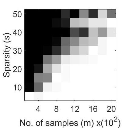 Figure 3
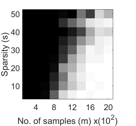 Figure 4
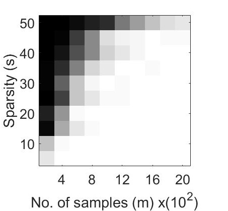 Figure 5
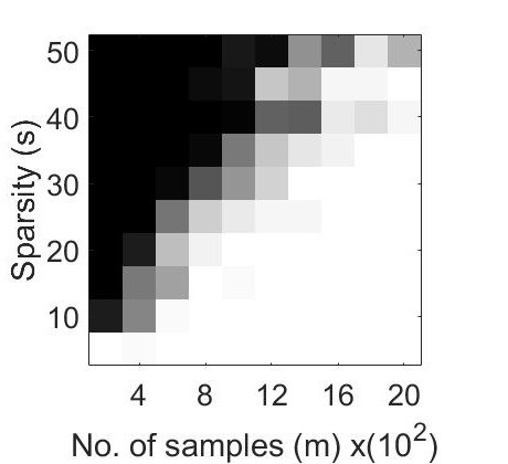 Figure 6
 Figure 7
 Figure 8
 Figure 9
 Figure 10
 Figure 11
 Figure 12
| Algorithm | CoPRAM | Block CoPRAM | SPARTA | ThWF |
|---|---|---|---|---|
| at phase trans | 1,600 | 1,400 | 1,800 | 2,000 |
| mean run time (s) | 0.4000 | 0.3258 | 0.3080 | 0.5808 |
Peer Reviews
No public reviews on file for this paper yet. If you reviewed it on a platform where reviews are public (OpenReview, ICLR, NeurIPS, ICML), you can paste yours below so the community can read it here.
Code & Models
Videos
No videos yet. Explain this paper in a talk, walkthrough, or lecture? Add one.
Sample-Efficient Algorithms for Recovering Structured Signals from Magnitude-Only Measurements
Gauri Jagatap and Chinmay Hegde The authors are with the Electrical and Computer Engineering Department at Iowa State University, Ames, IA 50010. Email: {gauri,chinmay}@iastate.edu. The authors thank Piotr Indyk and Thanh Nguyen for their helpful feedback. A conference version of this manuscript will appear in the Annual Conference on Neural Information Processing Systems (NIPS) in December 2017 [1]; this version has an expanded set of theoretical results as well as numerical experiments. This work is supported in part by the National Science Foundation under the grants CCF-1566281 and IIP-1632116.
Abstract
We consider the problem of recovering a signal , from magnitude-only measurements, for . This is a stylized version of the classical phase retrieval problem, and is a fundamental challenge in nano- and bio-imaging systems, astronomical imaging, and speech processing. It is well known that the above problem is ill-posed, and therefore some additional assumptions on the signal and/or the measurements are necessary.
In this paper, we consider the case where the underlying signal is -sparse. For this case, we develop a novel recovery algorithm that we call Compressive Phase Retrieval with Alternating Minimization, or CoPRAM. Our algorithm is simple and be obtained via a natural combination of the classical alternating minimization approach for phase retrieval with the CoSaMP algorithm for sparse recovery. Despite its simplicity, we prove that our algorithm achieves a sample complexity of with Gaussian measurements , which matches the best known existing results; moreover, it also demonstrates linear convergence in theory and practice. An appealing feature of our algorithm is that it requires no extra tuning parameters other than the signal sparsity level . Moreover, we show that our algorithm is robust to noise.
The quadratic dependence of sample complexity on the sparsity level is sub-optimal, and we demonstrate how to alleviate this via additional assumptions beyond sparsity. First, we study the (practically) relevant case where the sorted coefficients of the underlying sparse signal exhibit a power law decay. In this scenario, we show that the CoPRAM algorithm achieves a sample complexity of , which is close to the information-theoretic limit.
We then consider the case where the underlying signal arises from structured sparsity models. We specifically examine the case of block-sparse signals with uniform block size of and block sparsity . For this problem, we design a recovery algorithm that we call Block CoPRAM that further reduces the sample complexity to . For sufficiently large block lengths of , this bound equates to .
To our knowledge, our approach constitutes the first family of linearly convergent algorithms for signal recovery from magnitude-only Gaussian measurements that exhibit a sub-quadratic dependence on the signal sparsity level.
Index Terms:
Phase retrieval, sparsity, non-convex optimization, alternating minimization, structured sparsity, block-sparsity.
I Introduction
I-A Motivation
In this paper, we consider the problem of recovering a high-dimensional vector from (possibly noisy) magnitude-only linear measurements (or samples). That is, for , if
[TABLE]
then the task is to recover using the samples and the matrix .
Problems of this kind arise in numerous scenarios in machine learning, imaging, and statistics. For example, the classical problem of phase retrieval is encountered in imaging systems including diffraction imaging, X-ray crystallography, ptychography, and astronomical imaging [2, 3, 4, 5, 6]. For such systems, the physics of light acquisition are such that the optical sensors can only record the intensity of the light waves but not its phase. In terms of our setup, the vector would correspond to an image (possessing a resolution of pixels) and the measurements correspond to the magnitudes of its 2D Fourier transform coefficients. The goal is to stably recover the image from the measurements, ideally with as few observations (i.e., as small as possible).
Despite the prevalence of several heuristic approaches [7, 8, 9, 10] to solve (1), it is generally accepted that (1) is a very challenging nonlinear, ill-posed inverse problem both in theory and practice. Indeed, for generic and , one can show that (1) is NP-hard by reduction from certain well-known combinatorial problems [11]. Therefore, additional assumptions on the vector and/or the measurements are necessary.
A recent line of breakthrough results [12, 13, 14] have provided provably efficient algorithmic procedures for the special case where the measurement vectors are randomly drawn from certain multi-variate probability distributions (such as i.i.d. Gaussian distributions). By convention, we will continue to term such methods as “phase retrieval” algorithms. However, all these newer results require an “overcomplete” set of observations, i.e., the number of observations exceeds the problem dimension , sometimes by a significant amount. This requirement can pose severe limitations on computation, storage, and processing the measurements, particularly in the high-dimensional regime when and are very large. Our focus in this paper is to address the following:
Challenge: Can we solve the phase retrieval problem using very few samples (in particular, significantly fewer samples than the problem dimension)?
A possible solution to the above challenge is to leverage the fact that in many practical applications, often obeys certain low-dimensional structural assumptions. A common structural assumption used in imaging applications is that is -sparse in some known basis, such as the identity or the wavelet basis. For transparency, we assume that the sparsity basis is the canonical basis throughout this paper, unless otherwise specified. Similar structural assumptions form the core of sparse recovery, compressive sensing, and streaming algorithms [15, 16, 17], and it has been established that only samples are necessary for stable recovery of ; moreover, the dependence of the number of samples on and is information-theoretically optimal [18].
Solving the sparsity-constrained version of (1) (sometimes referred to as sparse phase retrieval in the literature) is therefore a natural next step, and numerous approaches have been proposed in this regard. These include a variant of alternating minimization [14], methods based on convex relaxation [19, 20, 21], and iterative thresholding-based techniques [22, 23]. However, all existing methods suffer from one (or more) of the following drawbacks:
Somewhat curiously, all of the above algorithms incur a sample complexity of for stable recovery, which is quadratically worse than the information-theoretic limit of 111Exceptions to this rule are the approaches of [24, 25, 26, 27, 28, 29], which indeed achieve near-optimal sample complexity and/or running time; however, these schemes are applicable only for very carefully designed measurements .. 2. 2.
Most algorithms suffer from a running time that is quadratic (or worse) in the dimension of the signal [19, 22]. 3. 3.
Many algorithms require stringent assumptions on the minimum (absolute) value of the nonzero signal coefficients [14, 23]. 4. 4.
Typically, these algorithms require tuning of several parameters for their proper functioning [19, 22, 23].
Finally, in specific applications, more refined structural assumptions on beyond sparsity are applicable. For example, point sources in astronomical images often produce clusters of nonzero pixels in a given image, while wavelet coefficients of natural images often can be organized as connected sub-trees. Algorithms that leverage such structured sparsity assumptions have been shown to achieve considerably improved sample-complexity in statistical learning and sparse recovery problems [30, 31, 32]. Indeed, a plethora of algorithms for modeling several types of structured sparsity constraints, including block-sparsity [31, 33], tree sparsity [34, 31, 35, 36], clusters [37, 33, 38], and graph-based models [39, 38, 40]. However, a systematic approach that leverage structured sparsity models in the context of phase retrieval does not seem to have been studied in the literature.
I-B Our contributions
In this paper, we establish a flexible algorithmic framework that systematically leverages (structured) sparsity-based signal models for the phase retrieval problem. We rigorously show that our approach matches the best available state-of-the-art sparse phase retrieval methods both from a statistical as well as computational viewpoint. Next, we show that it is possible to extend this algorithm to the case where the signal obeys certain types of block-sparsity structures, thereby further lowering the sample complexity of stable signal recovery.
We first consider the standard case where the underlying signal is -sparse (i.e. it has underlying model , where consists of all -sparse vectors of dimension ). For this case, we develop a novel recovery algorithm that we call Compressive Phase Retrieval with Alternating Minimization, or CoPRAM. Our algorithm is simple and be obtained via a natural combination of the classical alternating minimization approach for phase retrieval with the CoSaMP algorithm for sparse recovery, together with a smart initialization. Despite its simplicity, we prove that our algorithm achieves a sample complexity of with Gaussian sampling vectors in order to achieve linear convergence, which matches the best among all available existing results. An appealing feature of our algorithm is that it requires no extra a priori information other than the signal sparsity level , and that it requires no assumptions whatsoever on the nonzero signal coefficients. Finally, we show that our algorithm is stable with respect to noise in the measurements. To our knowledge, this is the first algorithm for sparse phase retrieval that simultaneously achieves all of the above properties. 222Note that we use the terms sparse phase retrieval and compressive phase retrieval interchangeably throughout the course of this paper.. 2. 2.
Next, following the setup of [20], we consider the case where the signal coefficients exhibit a power-law decay. Specifically, without loss of generality, suppose that the indices of are such that and . Then, we can prove that our CoPRAM algorithm exhibits a sample complexity of , which is very close to the information theoretic limit. 3. 3.
Finally, we consider the case where the underlying signal belongs to an a priori specified structured sparsity model. We specifically examine the case of block-sparse signals with uniform block size (i.e., the non-zeros can be equally grouped into non-overlapping blocks). We can equivalently say that the signal has underlying model . For this problem, we design a recovery algorithm that we call Block CoPRAM. We analyze this algorithm and show that leveraging block-structure further reduces the sample complexity of stable recovery to . For sufficiently large block lengths of , or block sparsity , this bound equates to which, again, is very close to the information theoretic limit. We also demonstrate that the more challenging case of overlapping blocks can also be solved using our technique, with a constant factor increase in sample complexity.
To our knowledge, this constitutes the first linearly convergent series of algorithms for phase retrieval where the (Gaussian) sample complexity has a sub-quadratic dependence on the sparsity level of the signal. A comparative description of the performance of our algorithms is presented in Table I.
I-C Techniques
Sparse phase retrieval. Our proposed CoPRAM algorithm is conceptually very simple. It integrates existing approaches in stable sparse recovery (specifically, the CoSaMP algorithm [41]) for sparse signal estimation with the alternating minimization approach for phase retrieval proposed in [14]333It is worthwhile to note that the high level idea of alternately estimating the phase and the signal is classical, dating back to the work of Gerchberg and Saxton [7]..
A similar integration of sparse recovery with alternating minimization was also introduced in the work of [14]; however, their approach only succeeds when the true support of the underlying signal is accurately identified during initialization. This can be fairly challenging to achieve in realistic situations when the signal coefficients are of differing magnitudes. Instead, CoPRAM permits the support of the estimate to evolve across iterations, and therefore can iteratively “correct” for any errors made during the initialization. Moreover, their analysis requires using fresh samples for every new update of the estimate, while our analysis succeeds in the (more practically useful) setting of using all the available samples at our disposal.
Our first challenge is to identify a good initial guess of the signal. As is the case with most non-convex algorithmic techniques, CoPRAM requires an initial estimate that is relatively close to the true vector . To this end, we use a variant of the spectral initialization procedure previously proposed in [23]. The basic idea is to identify “important” co-ordinates by constructing suitable biased estimators of each signal coefficient, followed by a specific eigendecomposition. However, the initialization in CoPRAM is far simpler than the approach in [23]; we perform no pre-processing of the measurements and our method requires no tuning parameters other than the sparsity level . We also provide a novel analysis of this modified initialization procedure. A drawback of the theoretical results of [23] is that they impose a minimum requirement on every non-zero entry of the true vector : . However, this assumption is equivalent to supposing that all nonzero coefficients are approximately the same magnitude, which can be unrealistic; in the case of real-world signal and image data, the (sorted) coefficients usually obey a power-law decay, which violates these constraints. Our analysis removes this requirement; the high level idea in our approach is to show that a coarse estimate of the support will suffice, since any errors in support identification necessarily have to coincide with small coefficients. Our approach also differs from the method adopted in [22], which selects indices corresponding to large coefficients based on a parameter-dependent threshold value. The support estimation step of our algorithm, coupled with the spectral decomposition method in [22] gives us a suitable initialization. We prove that the sample complexity for achieving this initial estimate of is , matching that of the best available previous methods.
Our next challenge is to show that starting from a good initial guess, an alternating procedure that switches between estimating the phases and estimating the sparse signal (using CoSaMP) converges rapidly to the desired solution. To this end, we unpack the analysis of the CoSaMP algorithm provided in [41]. In particular, we show that any “phase errors” made in the initialization step can be suitably controlled across different estimates. As a key step in our analysis, we leverage a recent result by [42] that shows sufficient decrease in the signal estimation error using the generic chaining technique of [43, 44]. Here too, our algorithm requires no tuning parameters other than the sparsity level .
Block-sparse phase retrieval. We can then use CoPRAM to establish its extension Block CoPRAM, which is a novel phase retrieval strategy for block sparse signals, which have been sampled using generic Gaussian measurements. Again, the algorithm is based on a suitable initialization followed by an alternating minimization procedure, and the algorithmic steps exactly mirror those of CoPRAM. To our knowledge, this is the first results for phase retrieval under more refined structured sparsity assumptions on the signal.
As above, the first challenge is to identify a good initial guess of the solution in the first stage. We proceed as in CoPRAM, but instead of identifying important co-ordinates, we instead isolate blocks of nonzero coordinates. The high level idea is to construct a different, specially chosen biased estimator for the “mass” of each block. We prove that a good initialization can be achieved using this procedure using only generic measurements. When the block-size is large enough, the sample complexity of the initialization can be sub-quadratic in the sparsity . Specifically, for the sample complexity is only a logarithmic factor away from the information-theoretic limit .
The second challenge is to demonstrate rapid descent to the desired solution in the second stage. To this end, we replace the CoSaMP sub-routine in CoPRAM with the model-based CoSaMP algorithm of [31], specialized to block-sparse recovery. The analysis proceeds analogously as above. To our knowledge, this constitutes the first end-to-end linearly convergent algorithm for phase retrieval (with generic Gaussian measurements) that demonstrates a sub-quadratic dependence on the sparsity level of the signal.
I-D Paper organization
The remainder of the paper is organized as follows. In Section II we provide a brief overview of prior work. In Section III, we present preliminaries and notation used for our analysis. In Sections IV and V, we introduce the CoPRAM and Block-CoPRAM algorithms respectively, and provide a theoretical analysis of their statistical as well as computational performance. In Section VI we provide a series of numerical experiments demonstrating the performance of our algorithms, and in Section VII we provide concluding remarks.
II Related work
II-A Prior work
The phase retrieval problem has received significant attention in the past few years. Attempts to solve this problem have mainly fallen into one of two broad solution approaches: convex and non-convex.
Convex approaches involve linearizing the problem by lifting the signal into a higher-dimensional space and solving a constrained optimization problem. Popular methodologies to solve the problem in the lifted framework include the seminal PhaseLift approach and its variations [12, 45, 46]; along similar lines is the PhaseCut approach [47] which proposes a phase retrieval approach based on an SDP relaxation of the MaxCut problem. However, most lifting based approaches suffer severely in terms of computational complexity. A recent convex approach that does not use the lifting procedure is PhaseMax, which produces a novel relaxation of the phase retrieval problem similar to basis pursuit [48]. While theoretically sound, the empirical performance of PhaseMax is not competitive with other lifting-based approaches.
On the other hand, nonconvex algorithms typically consist of two stages: finding a good initial point, followed by minimizing a loss function via a procedure similar to gradient-descent. The loss function being minimized can be either a function of a quadratic form involving the unknown signal, or a function involving the modulus of the inner products with the signal with the measurement vectors. Approaches based on Wirtinger Flow (WF) [13, 49, 22, 50] popularly use the quadratic form, while approaches based on Amplitude Flow (AF) [51, 23] as well as stochastic algorithms based on the Kaczmarz method [52] use the modulus form. In [53] Sun et al. describe a polynomial-time trust-region algorithm that uses arbitrary initializations to find the global optimum.
Recent works have adapted the phase retrieval framework for the case when the underlying signal is sparse. Some of the convex approaches include [19, 54], which uses a combination of trace-norm and -norm relaxation, to solve an SDP problem. Constrained sensing vectors have been used by Bahmani and Romberg [25] to effectively de-couple the problem into a phase retrieval stage followed by a sparse signal recovery stage, at optimal sample complexity of . Fourier measurements have been studied extensively in [55] in the convex setting. Similarly, non-convex approaches for sparse phase retrieval include [14, 23, 22] which achieve sample complexities of . Fourier measurements have been evaluated in the non-convex setting in [56], where they use a local search method to solve the sparse phase retrieval problem. Separate from this line of work, Schniter and Rangan in [57] have proposed an approximate message passing algorithm to experimentally exhibit a sample complexity of .
Going beyond sparsity, a natural approach is to refine the assumptions on the nonzero signal coefficients so as to better model various types of real-world phenomena. Structured sparsity models have been proposed to leverage combinatorial interactions such as groups, blocks, clusters, trees, and various other refinements that can be used to model the signal of interest. Applications of structured sparsity models have been developed for sparse recovery [31, 32, 39, 38, 40, 58, 34, 31, 35, 36] as well as in high-dimensional optimization and statistical learning [30, 33]. However, to the best of our knowledge, there has been no rigorous results that explore the impact of structured sparsity models for the phase retrieval problem.
II-B Subsequent work
Since the initial appearance of this paper on Arxiv and its subsequent conference publication [1], numerous related works have emerged. Of notable interest has been Waldsperger’s new result for phase retrieval which shows that standard alternating minimization provably converges without any special initialization, albeit with much higher sample complexity [59]. At the moment, we do not know how to design initialization-free algorithms in the case of sparse phase retrieval, and leave that as potential future work. Other recent works include re-weighted amplitude flow [60] and convolutional phase retrieval [61]. Our framework proposed in this paper has also spurred follow-up work in an optical imaging application called Fourier ptychography with promising results; see [62, 63] for details.
III Preliminaries
We introduce some notation that will be used throughout the paper. We use bold capital-case letters (, etc.) to denote matrices, bold small-case letters (, etc.) to denote vectors, and non-bold letters ( etc.) for scalars. We use and to denote the transpose of the vector and the matrix respectively. The diagonal matrix form of a column vector is represented as diag, which is the matrix in with its diagonal elements as and all off-diagonal entries are zero. The cardinality of set is expressed using the operator .
In this paper we use the standard Gaussian (or normal) distribution over (i.e., the elements of are distributed according to the distribution ). We define for every , with the convention that . Also, we define for every . The projection of vector onto a set of coordinates is represented as , . Projection of matrix onto is , . For the sake of improved computational complexity, for algorithmic implementations, can be assumed to be a truncated vector , discarding all elements in . The element-wise inner product of two vectors and is represented as . has been used to denote unspecified constants that are large enough. Similarly has been used for small constants. The abbreviations wlog and whp denote “without loss of generality” and “with high probability” respectively.
IV Compressive phase retrieval
In this section, we propose a new algorithm for solving the sparse phase retrieval problem and analyze its performance. Later, we will show how to extend this algorithm to the case of more refined structural assumptions about the underlying sparse signal.
We first provide a brief outline of our proposed algorithm. It is clear from the discussion in the introduction that the recovery problem (1) is highly non-convex, and multiple locally optimal solutions might exist. Therefore, as is typical in modern non-convex methods [14, 23, 64] we use an spectral technique to obtain a good initial estimate. This technique itself is a modification of the initialization stage of Algorithm 1 of [23]; however, as we discuss below, our method requires no special tuning parameters except for knowledge of the underlying sparsity . Moreover, in contrast with [23] our theoretical analysis requires no extra assumptions on the signal coefficients.
Once an appropriate initial estimate is chosen, we then show that a simple alternating-minimization algorithm will converge rapidly to the underlying true signal. Our proposed algorithm is new, and builds upon the original alternating-minimization algorithm proposed in [14]. In a departure from existing sparse phase retrieval methods [23, 22], our method is parameter free except for knowledge of the sparsity level .
We call our overall algorithm Compressive Phase Retrieval with Alternating Minimization (CoPRAM). As described above, the algorithm is divided into two stages: an Initialization stage and a Descent stage. The stages are presented in pseudocode form as Algorithms 1 and 2.
IV-A Initialization
The first stage of CoPRAM uses a similar approach as those provided in previous sparse phase retrieval methods. The high level idea is to use the measurements to construct a biased estimator of the (squared) absolute values of the true signal coefficients. For the signal coefficient, the marginal is given by:
[TABLE]
and the set of all ’s can be calculated in time. The marginals themselves do not directly produce the signal coefficients, but the “weight” of each marginal (with sufficiently many samples) can enable identification of the coordinates of the true signal support. Once the support is accurately identified, a spectral technique (e.g., the methods of [14, 23, 22]) can be used to construct a good initial estimate .
However, accurate support identification can be tricky in general, particularly in the presence of very small signal coefficients. Indeed, to avoid this issue, earlier works [14, 23] assume that the magnitudes of the nonzero signal coefficients are all sufficiently large, i.e., . As discussed earlier, this assumption can be unrealistic, violating the power-decay law.
Our analysis resolves this issue by relaxing the requirement of accurately identifying the support. The basic intuition is that even a coarse estimate of the support suffices to achieve a good estimate, since the errors are all going to correspond to small coefficients anyway. Such “noise” in the signal estimate can be controlled with a sufficient number of samples. A similar argument has been made in the analysis of the initialization stage of [22]; however, their estimate is a strict subset of the true support and their method requires tuning of real-valued parameters that can be hard to estimate in practice. Instead, we use a simpler estimation procedure. Indeed, we show that a simple pruning step that rejects the smallest coordinates, followed by the spectral procedure of [23], gives us the initialization that we need.
Concretely, we leverage the following fact: if elements of are distributed as per standard normal distribution , a weighted correlation matrix can be constructed with diagonal elements ,
[TABLE]
Then the expectation of this matrix is,
[TABLE]
where . The diagonal elements of this expectation matrix are given by:
[TABLE]
Intuitively, the signal marginals at locations on the diagonal of corresponding to are larger, on an average, than those corresponding to the zero-locations . Using this as the baseline, we evaluate the diagonal elements of the matrix (which we refer to as marginals) and establish a threshold value which separates the indices corresponding to these marginals into sets and .
We formalize the above argument. Our first result shows that given a sufficient number of measurements of the form (5), this method produces an estimate that is close enough to the true underlying signal.
Theorem IV.1**.**
The output of Algorithm 1, is a small constant distance away from the true signal , i.e.,
[TABLE]
as long as the number of (Gaussian) measurements ‘m’ satisfies the following bound,
[TABLE]
with probability greater than .
This theorem is proved via Lemmas A.1 through A.4, and the argument proceeds as follows. We evaluate the marginals of the signal , in broadly two cases: and . The key idea is to establish one of the following:
If there is a restriction on the minimum element of the true (i.e., if it is bounded away from zero by a specific amount), then there exists a clear separation between the marginals for and , with high probability. Then one would, whp, pick up the correct support in Algorithm 1 (i.e. ). The top-singular vector of the truncated matrix gives a good initial estimate . 2. 2.
If there is no such restriction, even then the support picked up in Algorithm 1, , contains a bulk of the correct support . Some fraction of the elements picked up in are incorrect, but we prove that they induce negligible error in estimating the initial vector .
These approaches are illustrated in Figures 7 and 8 in Appendix A. The marginals for are upper bounded as stated in Lemma A.1. Similarly, the marginals for are lower bounded as stated in Lemma A.2. The identification of the support (which provably contains a significant chunk of the true support ) serves as a basis to construct the truncated correlation matrix . The top singular vector of this matrix , gives us a good initial estimate of the true signal .
The final step of Algorithm 1 requires a scaling by a factor . This ensures that the power of the initial estimate is close to the power of the true signal (this is required because the calculation of the top-singular vector gives us a normalized vector ). Provided sufficiently many samples, the signal power is well approximated by the average power in the measurements which is defined as
[TABLE]
Using Lemma F.1 in Appendix F we can show that
[TABLE]
for small constant with probability greater than .
IV-B Descent to optimal solution
Once we obtain a good enough initial estimate such that , whp, we now construct a method to accurately recovery the true . To achieve this, we adapt the alternating minimization approach from [14].
We introduce some notation. The observation model in (1) can be restated as follows:
[TABLE]
for all . We denote the phase vector as a vector that contains the (unknown) signs of the measurements, i.e., for all . We can also define a diagonal phase matrix , such that . Then our measurement model gets modified as:
[TABLE]
where denotes the true phase matrix. Consider minimizing the loss function composed of two variables and ,
[TABLE]
Note that the problem above is not convex, because is restricted to be a diagonal matrix , where is a set of all diagonal matrices with diagonal entries constrained to be in . Instead, we alternate between estimating and . We perform two estimation steps:
If we fix the signal estimate , then the minimizer is given in closed form as:
[TABLE]
We call this the phase estimation step. 2. 2.
If we fix the phase matrix , the signal vector can be obtained by solving a sparse recovery problem,
[TABLE]
if (and each entry of , is sampled from independent Gaussian , such that satisfies the restricted isometry property). We call this the signal estimation step.
We employ the CoSaMP [41] algorithm to (approximately) solve (9). Note that since (9) itself is a non-convex problem and exact minimization can be hard. However, we do not need to explicitly obtain the minimizer but only show a sufficient descent criterion, which we achieve by performing a careful analysis of the CoSaMP algorithm. For analysis reasons, we require that the entries of the input sensing matrix are distributed according to . This can be achieved by scaling down the inputs to CoSaMP: by a factor of (see -update step of Algorithm 2). Another distinction is that we use a “warm start” CoSaMP routine for each iteration where the initial guess of the solution to (9) is given by the current signal estimate.
We now analyze our proposed descent scheme. We obtain the following theoretical result:
Theorem IV.2**.**
Given an initialization satisfying , for , if we have number of (Gaussian) measurements , then the iterates of Algorithm 2 satisfy:
[TABLE]
where is a constant, with probability greater than , for positive constant .
The proof of this theorem can be found in Appendix C.
Combining both stages, the number of measurements are required to obey the following lower bound:
[TABLE]
for the overall CoPRAM algorithm to succeed.
IV-C Robustness to noise
The above analysis assumes that the measurements are pristine (noiseless). We can also demonstrate that the CoPRAM algorithm are sufficiently robust in the presence of noise. This is established in the following theorem.
Theorem IV.3**.**
Given Gaussian measurements , CoPRAM can recover the model sparse signal from noisy measurements of the form
[TABLE]
where is a scaled sub-exponential. This retains the previously derived expression for sample complexity as in Theorem IV.1 up to a constant factor. The algorithm converges according to the iteration invariant:
[TABLE]
where is the number of outer iterations of CoPRAM and Block CoPRAM, and .
The proof for this theorem can be found in Appendix D. An identical analysis holds for the block-sparse case which we elaborate in more detail below.
IV-D Sparse signals exhibiting power law decay
The quadratic dependence of the sample complexity on the signal sparsity level , as derived in Theorem IV.1, is typical (and also shared by the other works [49, 23]) but somewhat problematic. In particular, if the signal sparsity exceeds the square-root of the dimension , the result becomes moot and one may as well as standard phase retrieval techniques!
In this section, we demonstrate a method to break through this quadratic barrier, albeit under somewhat more stringent assumptions on the signal. Specifically, we analyze the scenario hypothesized in [20] in which the signal follows a power-law decay. That is, suppose that the signal coefficients have been suitably re-indexed such that , for can be arranged in non-increasing order:
[TABLE]
where and . Due to the isotropic nature of the Gaussian measurement scheme, such a re-indexing can be assumed without loss of generality.
We can show that this extra power-law decay assumption results in far fewer samples, for the CoPRAM initialization step to achieve a sufficiently good initial guess. Combined with Theorem IV.2, we obtain the following result:
Theorem IV.4**.**
Given Gaussian measurements , then CoPRAM can recover the -sparse signal , with , where is the number of outer iterations of CoPRAM, from measurements, as long as the coefficients of the signal follow a power-law decay as described in (12).
The proof for this theorem can be found in Appendix E.
V Block-sparse phase retrieval
The analysis of the proofs mentioned so far, as well as experimental results suggest that we can reduce sample complexity for successful sparse phase retrieval by exploiting further structural information about the signal. We assume that the true signal , is block sparse with uniform block length and effective block sparsity . We introduce the concept of block marginals, a block-analogue to signal marginals, which can be analyzed to crudely estimate the block support of the signal in consideration. We use this formulation, along with the alternating minimization approach that uses model-based CoSaMP [31] to descend to the optimal solution. In the next subsections, we discuss the initialization and descent of the Block CoPRAM algorithm. The pseudo-code for Block CoPRAM is stated in Algorithms 3 and 4.
V-A Initialization
Block-sparse signals , can be said to be following a sparsity model , where describes the set of all block-sparse signals with non-zeros being grouped into uniform pre-determined blocks of size , such that block-sparsity . The effective sparsity of the signal is still , however the non-zero elements are constrained to appear in blocks. We use the index set , to denote block-indices.
Analogous to the concept of marginals defined above, we introduce block marginals , where is defined as in (2). For block index , we define:
[TABLE]
to develop the initialization stage of our Block CoPRAM algorithm. Similar to the proof approach of CoPRAM, we show that there exists a threshold that separates the block marginals , for and , for respectively. Here, represents the “block support”, i.e., the set of active block-indices. We can then evaluate the block marginals, and use the top- such marginals to obtain a crude approximation of the true block support . This support can be used to construct the truncated correlation matrix . The top singular vector of this matrix gives a good initial estimate for the Block CoPRAM algorithm (Algorithm 4). Through the evaluation of block marginals, we proceed to prove that the sample complexity required for a good initial estimate (and subsequently, successful signal recovery of block sparse signals) is given by . This essentially reduces the sample complexity of signal recovery by a factor equal to the block-length over the sample complexity required for standard sparse phase retrieval.
Formally, we obtain the following result:
Theorem V.1**.**
The initial vector , which is the output from Algorithm 3, is a small constant distance away from the true signal , i.e.
[TABLE]
for , as long as the number of measurements satisfy
[TABLE]
with probability greater than .
The proof can be found in Appendix B, and carries forward intuitively from the proof of the sparse phase-retrieval framework.
V-B Descent to optimal solution
For the descent of Block CoPRAM to optimal solution, the phase-estimation step is the same as that in CoPRAM (8). For the signal estimation step, we attempt to solve the same minimization as in (9), except with the additional constraint that the signal is block sparse,
[TABLE]
where describes the block sparsity model. In order to approximate the solution to (14), we use the model-based CoSaMP approach of [31]. This is a straightforward specialization of the CoSaMP algorithm and has been shown to achieve improved sample complexity over existing approaches for standard sparse recovery.
Similar to Theorem IV.2 above, we obtain the following result:
Theorem V.2**.**
Given an initialization , satisfying , where , if we have number of measurements , then the iterates of Algorithm 4 satisfy:
[TABLE]
where is a constant, with probability greater than , for positive constant .
The proof of this theorem can be found in Appendix C.
V-C Extension to blocks of non-uniform sizes
The analysis so far has been made for uniform blocks of size . However the same algorithm can be extended to the case of sparse signals with non-uniform blocks. Such a model is particularly useful for time-series signals where the nonzeros occur in “bursts” of variable lengths and start times.
Formally, consider the clustered sparsity model for 1D signals in , comprising signals with non-zeros that occur in no more than non-overlapping blocks (clusters), each of which exhibit potentially unknown sizes and locations. The above analysis does not immediately apply to this case; however, by the analysis approach of [37], we can show that any such clustered-sparse signal with parameters can be simulated using a uniform block-sparse signal with parameters . Therefore, the only price to be paid is a tripling of the block sparsity parameter . Provided we are willing to tolerate this increase, we can use exactly the same Block CoPRAM algorithm (including both the initialization as well as the descent stages) as described above, with only a constant factor increase in the sample complexity.
We note that this argument is only applicable to block-sparse 1D signals (such as time-domain signals); extending this argument to general clustered-sparse images and higher-dimensional data is much more involved, and we leave this to future work.
VI Numerical experiments
In this section, we present the results of a range of simulations supporting our algorithms and demonstrate their benefits over the state-of-the-art in sparse phase retrieval. All numerical experiments were conducted using MATLAB 2016a on a desktop computer with an Intel Xeon CPU at 3.3GHz and 8GB RAM.
Our experiments explores the performance of the CoPRAM and Block CoPRAM algorithms on synthetic data. The non-zero elements of the test signal , with are generated using zero-mean Gaussian distribution and normalized, such that . The elements of sensing matrix , are also generated using the zero-mean Gaussian distribution . The sparsity levels are chosen in steps of with a maximum value of such that (for values of , the effect of sparsity is minimal and standard non-sparsity based phase retrieval algorithms perform equally well). A block length of is considered for all generated signals in experiments in Figures 2, 1 and 4. The number of measurements is swept from to in steps of . We repeated each of the experiments (fixed ) in Figures 2, 1 and 4 for independent Monte Carlo trials, and the experiments in Figure 3 for independent Monte Carlo trials.
For our simulations, we compared our algorithms CoPRAM and Block CoPRAM with two other sparse phase retrieval algorithms: Thresholded Wirtinger Flow [22] and SPARTA [23]. For our set of generated signals, the AltMinSparse method mentioned in [14] does not recover the signal in most cases (if the initialization stage fails to pick the correct support, the subsequent AltMinPhase procedure can never give a good solution). We therefore do not include this algorithm for comparisons.
For Thresholded WF, we set parameters which were optimized based on a number of trial cases and were kept constant throughout all experiments, with values , and . Similarly, for SPARTA, we set the parameters to be , and as mentioned in their paper.
For the first experiment, we generated phase transition plots by evaluating the probability of successful recovery, i.e. number of trials out of , that gave a relative error in retrieval . We let each of the algorithms to run for a total of iterations. The recovery probability for varying values of and has been illustrated in Figure 1 through phase transition diagrams. It can be noted that CoPRAM (2 (c)) and SPARTA (2 (b)) perform comparably, while Block CoPRAM (2 (d)) performs the best among all four algorithms, in terms of sample complexity.
The phase transition graphs for and for the four algorithms is displayed in Figure 2.
It can be noted that increasing the sparsity of signal shifts the phase transitions to the right (sample complexity of has a quadratic dependence on for CoPRAM, SPARTA and Thresholded WF). However the phase transition for Block CoPRAM has a less apparent shift, as compared to other algorithms (sample complexity of has sub-quadratic dependence on ). It can be noted that as sparsity increases, the gap between the phase transition of Block CoPRAM and other algorithms in consideration, increases. As demonstrated in Figure 1, the Block CoPRAM approach exhibits lowest sample complexity for the phase transitions in both cases (a) and (b) of Figure 2.
The mean running time of the algorithms for different algorithms is tabulated in Table II. It can be noted that the running times of our algorithms CoPRAM and Block CoPRAM are at par with SPARTA and Thresholded WF.
Leveraging block-sparsity. For the second experiment, we study the variation of phase transition with block-length, for Block CoPRAM (refer Figure 3). For this experiment we fixed a signal of length , sparsities for a block length of . We observed that the phase transitions improve with increase in block length (used to estimate the signal in the algorithm) up to a point. At block sparsities and , there is little difference in the phase transitions, as the regime of the experiment is very close to the information theoretic bound of .
Effect of noise. For our third experiment, we study the effect of noise on the measurements of the form:
[TABLE]
for , to verify the claims in Theorem IV.3. The noise vector is sampled from a zero-mean Gaussian distribution , where is determined using the input noise-signal-ratio (NSR). We compared CoPRAM, Block CoPRAM and SPARTA to analyze robustness to noisy measurements for amplitude only measurements (ThWF is excluded because they use quadratic measurements). We vary the input NSR , from to in steps of . We fix signal parameters and number of measurements to . This experiment was run for independent Monte Carlo trials. The variation of mean relative error can be seen in Figure 4. We observe that Block CoPRAM exhibits greater robustness to noise compared to CoPRAM and SPARTA in all cases considered.
Power-law decay. For our fourth experiment, we verify the claims in Theorem IV.4. We set the signal length to . We analyze the effect of power law decay on signals with sparsities and for different rates of decay and compare this to the case with no power law decay (coefficients picked random normally). We observe an improvement in sample complexity with respect to the ”no powerlaw decay” case, as seen in Figure 5. The improvement is more prominent as we increase the sparsity from to .
Experiments on real images. For our final experiment, we evaluated the performance of our algorithm on a real image, with induced sparsity in the wavelet basis (db1). We used a image of Lovett Hall, and used the thresholded wavelet transform (using Haar wavelet) of this image as the sparse signal with . This image was reconstructed using samples, using CoPRAM and the standard AltMinPhase algorithm described in [14]. We used signal-to-noise ratio (SNR) to quantify quality of reconstruction. In Figure 6, we demonstrate how enforcing a sparsity constraint enables recovery of the same image using fewer samples and better reconstruction quality.
VII Discussion
In this paper, we have introduced a set of new algorithmic approaches for sparse as well as structured sparse phase retrieval. Our algorithms are conceptually simple and indeed are reminiscent of classical heuristics for phase retrieval; however, our analysis also shows an asymptotic reduction in sample complexity when additional structures on top of standard sparsity are leveraged within the reconstruction process. Several open questions remain, including expanding our analysis to more sophisticated sparsity models, such as clusters, trees, groups, and graphical models [58]. Moreover, our analysis only applies to the case of Gaussian samples, and extending our results to more realistic measurement schemes such as Fourier samples and coded diffraction patterns [46] will be an interesting direction of future study; indeed, our preliminary experimental results in [62, 63] have shown the empirical benefits of our algorithms for such challenging measurement setups.
Appendix A CoPRAM Initialization
In this section we state the proofs related to the initialization in Algorithm 1, for compressive phase retrieval. This includes the proofs of Lemmas A.1 - A.4 which complete the proof of Theorem IV.1.
The outline of the proof is sketched out as follows. Using Lemma A.1, we can find an upper bound on marginals for . Consequently,
[TABLE]
with probability greater than . Marginals for can be evaluated in two ways:
Assuming a bound on the minimum element of : . The proof then carries forward from the work in [23], where they arrive at the lower bound on the minimum marginal for , with probability greater than ,
[TABLE]
given that . This proof is similar to that mentioned in Lemma A.2. Piecing these two together,
[TABLE]
which implies that the support picked up using the top -marginals is the true support with probability greater than , given , as long as there is a clear separation between and . They proceed to show that with a high probability, , using Proposition 1 of [51], completing the proof of Theorem IV.1. 2. 2.
If there is no such assumption on the minimum entry , we proceed with a longer proof, as stated below using Lemmas A.2-A.4. The idea is to show that and subsequently , effectively implying that .
This idea and the partition of support sets used in the proof have been illustrated in Figures 7 and 8.
Lemma A.1**.**
For all , with probability greater than , the corresponding marginals are upper-bounded as
[TABLE]
Proof.
Evaluating the marginals:
[TABLE]
where is independent of for all . Evaluating the tail bound in terms of a series of tail bounds for independent random variables and , one can use Lemma 4.1 of [65] for the variables with weights (here ):
[TABLE]
Further, using the Chebyshev’s inequality for :
[TABLE]
Using the Gaussian tail bound for followed by union bound:
[TABLE]
With probability at most , for each , using a union bound on these three tail bounds,
[TABLE]
Using a union bound for all ( such), with probability at least ,
[TABLE]
Using Lemma F.1, for , and using the fact that :
[TABLE]
which establishes the upper bound on marginals associated with the zero-locations , with probability greater than . ∎
Lemma A.2**.**
For , with probability greater than , the corresponding marginals are lower-bounded as
[TABLE]
where is defined as
[TABLE]
Subsequently, we can define as
[TABLE]
with and forming a partition of and the corresponding energy in the elements is lower-bounded as
[TABLE]
Proof.
Evaluating the marginals:
[TABLE]
For , and are dependent random variables. The marginal can be evaluated through a concentration bounds on the two terms that compose the RHS of (23): and . This can be done by evaluating the expectation values:
[TABLE]
Constructing variable which is upper bounded, with zero mean and bounded variance, we can use Lemma F.3 to establish a concentration bound with parameters:
[TABLE]
Using Lemma F.3, for each ,
[TABLE]
This requires . This establishes the bound on the first term . Similarly, we can establish a bound on the second term , which requires Lemma 4.1 of [65], with probability greater than , for each :
[TABLE]
for . Combining these two concentration bounds (24), (25), taking a union bound for all and substituting in (23):
[TABLE]
which holds with probability at least .
If the set , is constructed as in (20), then evaluating the bound in (26), we get:
[TABLE]
holds for all elements , with probability greater than , yielding the bound in (19). ∎
Lemma A.3**.**
If is chosen as in Algorithm 1, with probability greater than ,
[TABLE]
as long as the number of measurements follow the following bound
[TABLE]
Proof.
If is chosen such that it corresponds to the top- marginals , then it will pick up corresponding to large marginals , and corresponding to small marginals ( form a partition of and , refer Figure 8 for illustration of the sets):
[TABLE]
By definition and therefore . If we can prove that and , then we can claim that . First, we prove that :
[TABLE]
By construction, and form a partion of :
[TABLE]
Using (22), we compute the bound,
[TABLE]
since there are at most elements in , which is the required condition (27). This requires sample complexity to satisfy:
[TABLE]
∎
We have proved that . Now we need to prove that , which we do using Lemma A.4.
Lemma A.4**.**
With probability greater than
[TABLE]
as long as the number of measurements follow the following bound
[TABLE]
Proof.
The top singular vector of is equal to true , from (3):
[TABLE]
We then define and is the top singular vector of .
Defining , where , then, , and,
[TABLE]
At this stage, we can invoke the proof idea from [22], as stated in Lemma F.2 from Appendix F, to give the following bound,
[TABLE]
with probability at least , as long as . Now we can use the fact that , so that,
[TABLE]
Since can be seen as a perturbation of , where the top two singular values of are spaced apart, we can use the Sin-Theta theorem [66] to bound the difference between the normalized top-singular vectors of and of as,
[TABLE]
Hence, with probability greater than , Lemma A.4 holds. ∎
Combining Lemmas A.3 and A.4, we have the final result:
[TABLE]
as long as the number of measurements follow the bound in (28). Hence the initial vector is upto a constant factor away from the true vector . The constant can be decreased by increasing the number of samples (see equation (31)). This completes the proof of Theorem IV.1.
Appendix B Block CoPRAM initialization
In this section we state the proofs related to the initialization for Block CoPRAM in Algorithm 3, for block sparse signals.
We prove theorem V.1 for the initialization stage of Block CoPRAM as follows.
See V.1
Proof.
Evaluating the marginals , for all , from (16), with probability greater than , we have:
[TABLE]
Evaluating the block marginals , for , we use a modification of (24), with probability less than ,
[TABLE]
Rearranging the terms,
[TABLE]
where the final expression holds with probability less than . Here, we have used he shorthand . Finally, taking a minimum over all such block marginals , with probability greater than ,
[TABLE]
if . Assuming that , the following holds
[TABLE]
Equating the expression for probability,
[TABLE]
which puts a bound on the block marginals for .
Hence, as long as , there is a clear separation in the marginals, using (33) and (32),
[TABLE]
where is large enough. Given that there is a clear separation in the marginals, the block support as picked up as in Algorithm 3, is exactly the true block support .
It is then straightforward to show that the top singular vector of the truncated covariance matrix is actually close to the true block sparse vector , which holds with probability greater than .
Thus far, the proof requires an assumption on . We do away with this assumption as follows:
For evaluating block marginals for , we can use the result of Lemma A.1, to obtain the same bound as in (32), with probability greater than ,
[TABLE]
For evaluating block marginals for we can use equations (20) and (21), and extend this model of signal supports to block supports defined as:
[TABLE]
Using equation (26), and LHS of (45),
[TABLE]
Constructing block marginals as ,
[TABLE]
We can then extend the proof of Lemma A.3 to give the partitions,
[TABLE]
and the inequalities:
[TABLE]
This inequality gives us a bound on the number of measurements , similar to (31),
[TABLE]
with probability greater than . This gives us the evaluation of block-marginals for and , respectively. It is then straightforward to show that the top singular vector of the truncated covariance matrix , given is actually close to the true block sparse vector with probability greater than . ∎
Appendix C CoPRAM and Block CoPRAM descent
In this section we state the proofs related to the descent to optimal solution in Algorithm 2 (CoPRAM), for sparse signals and Algorithm 4 (Block CoPRAM), for block sparse signals. This includes the proof of Theorem IV.2 and Theorem V.2. We prove theorem IV.2 to show descent of the CoPRAM algorithm, as follows.
Note: For evaluation of the distance measure , we only consider , assuming that at the end of initialization stage. We claim that wlog, the same results would hold, if .
See IV.2
To show the descent of our alternating minimization algorithm using CoSaMP, we need to analyze the reduction in error, per step of CoSaMP, (refer Algorithm 5) first:
[TABLE]
where corresponds to the ’th run of CoSaMP for the update of . Using RIP of ,
[TABLE]
with high probability, where is the RIP constant. Now, analyzing the inputs to CoSaMP, in step 4 of Algorithm 2,
[TABLE]
where , is error due to failure in estimating the correct phase.
Using equation (36) and substituting into equation (35), the per-step reduction in error for each run of CoSaMP is:
[TABLE]
where the first step is from using triangle inequality, the second step is from using the fact that is exactly -sparse with support . The third step is using the fact that truncation of in , is the minimizer of the LS problem , the fourth step uses (36) again, the final step uses RIP again (which holds with probability greater than , with being a positive constant).
Finally, the first term in the previous inequality can be bounded using (Lemma 4.2 of CoSaMP [41], refer Lemma F.4), to yeild,
[TABLE]
where are as stated in Lemma F.4. Assuming that CoSaMP is let to run a maximum of iterations,
[TABLE]
The second part of this proof requires a bound on the phase error term :
[TABLE]
We proceed to finish this proof by invoking Lemma C.1.
Lemma C.1**.**
As long as the initial estimate is a small distance away from the true signal ,
[TABLE]
and subsequently,
[TABLE]
*then the following bound holds, *
[TABLE]
with probability greater than , where is a positive constant, as long as . We can use this to bound the phase error as,
[TABLE]
where , .
This proof has been adapted from Lemma 7.19 of [42] and uses the generic chaining techniques of [43, 44]. Using this in addition to equation (37), we have our final per-step error reduction for a single run of CoPRAM (Algorithm 2), as:
[TABLE]
where .
Evaluating convergence parameter :. To obtain per-step reduction in error, we require . For sake of numerical analysis, , then . Let , then . Similarly, and . Suppose CoSaMP is allowed to run for iterations then, .
The inequalities used for CoSaMP, particularly (34) can be made tighter, which would give less tight restrictions on the factor , that controls how close the intial estimate is to the true signal .
We now restate theorem V.2 for Block CoPRAM as follows.
See V.2
The proof for this is a natural extention to the one we have proved in Theorem IV.2, and would use the results from the paper on model-based compressive sensing [31], wherever Block CoSaMP is invoked.
Appendix D Noise robustness
In this section, we show that both CoPRAM and Block CoPRAM are robust to noise, and establish the proof of Theorem IV.3.
See IV.3
We assume the modified version of (1) acquisition model:
[TABLE]
where is distributed according to a scaled sub-exponential random variable. If the variance of the noise is much smaller in comparison to the magnitude of the measurements, then the following approximation holds:
[TABLE]
where are sub-exponentail random variables (special case is Gaussian with distribution ).
D-A CoPRAM Initialization
The marginals used for initialization will get modified as:
[TABLE]
Similarly signal power gets modified as:
[TABLE]
Then much of the analysis for the initialization, follows from [22]. Key points in the proof stated in Appendix A get modified as follows:
Lemma (A.1)
[TABLE]
where the second term is bounded as Equation (6.4) in [22] as
[TABLE]
with probability greater than and the first term is bounded using (18).
Since we have assumed that the noise variance is much lesser than the signal power, . Hence, the new marginal threshold for is:
[TABLE]
with probability greater than .
Lemma (A.2) Similarly, is lower bounded for , using (26) along with Equation (6.4) in [22]:
[TABLE]
where we redefine and as
[TABLE]
Subsequently, we can define as
[TABLE]
Lemmas (A.3) and (A.4) hold using these modifications, upto a constant factor. Theorem IV.1 holds with probability greater than .
D-B CoPRAM Descent
In the Descent stage, apart from the phase estimation error and signal estimation error, we also have an additional measurement error term. This modification reflects in Equation (36) of Appendix C as:
[TABLE]
where is the measurement error. This error propagates to modify Equation (37) as:
[TABLE]
Finally, the main convergence result from Equation (38) gets modified as:
[TABLE]
where . After a total of iterations of CoPRAM, we get the convergence result:
[TABLE]
Thus the quality of reconstruction depends on level of input noise , which is bounded with high probability.
Appendix E Power law decay
In this section we state the proof of the sample complexity required for sparse signals following power-law decay, as described in Theorem IV.4. See IV.4 Note that a power-law decaying signal can be normalized as follows:
[TABLE]
where is an indicator of the tightness of power-law inequality.
Additionally, we can find the index at which all power-law decaying signal elements fall bellow threshold :
[TABLE]
The task is to find a tighter bound for , as compared to (30). This bound can be established using our additional assumption of power law decay. We analyze this bound using the threshold criteria , as in (20) and :
[TABLE]
where we have used (44) and the fact that .
In this regime, the sample complexity for the overall algorithm is dominated by the sample complexity for the descent stage ( = max(,)).
Appendix F Supplementary theorems
In this section we state some of the lemmas with or without proofs, used in Appendices A and C.
Lemma F.1**.**
With probability of at least ,
[TABLE]
Proof.
Rotational invariance property of Gaussian distributions imply that has the same distrubution as . Using Lemma 4.1 of [65] on , we can obtain the upper bound,
[TABLE]
Similarly, we can obtain the lower bound,
[TABLE]
The signal power is then bounded from below as
[TABLE]
and similarly, it is bounded from above as,
[TABLE]
with probability at least , for , large enough. If , then the bounds are,
[TABLE]
where . ∎
Lemma F.2**.**
With probability at least , the following holds,
[TABLE]
where , provided .
This proof has been adapted from Lemma A.6 of [22].
Lemma F.3**.**
Suppose are i.i.d. centered, bounded real-valued random variables obeying
[TABLE]
with cumulative distribution function of the standard normal distribution being denoted as
[TABLE]
*then *
[TABLE]
This establishes the tail probability of martingale with differences bounded from one side [67].
Lemma F.4**.**
The -sparse residual error can be upper bounded as,
[TABLE]
where and .
This lemma has been adapted from Lemmas 4.2 and 4.3 of [41].
The reference list from the paper itself. Each links out to its DOI / PubMed record.
- 1[1] G. Jagatap and C. Hegde. Fast, sample-efficient algorithms for structured phase retrieval. In Adv. Neural Inf. Proc. Sys. (NIPS) , pages 4922–4932, 2017.
- 2[2] Y. Shechtman, Y. Eldar, O. Cohen, H. Chapman, J. Miao, and M. Segev. Phase retrieval with application to optical imaging: a contemporary overview. IEEE Sig. Proc. Mag. , 32(3):87–109, 2015.
- 3[3] R. Millane. Phase retrieval in crystallography and optics. JOSA A , 7(3):394–411, 1990.
- 4[4] A. Maiden and J. Rodenburg. An improved ptychographical phase retrieval algorithm for diffractive imaging. Ultramicroscopy , 109(10):1256–1262, 2009.
- 5[5] R. Harrison. Phase problem in crystallography. JOSA a , 10(5):1046–1055, 1993.
- 6[6] J. Miao, T. Ishikawa, Q Shen, and T. Earnest. Extending x-ray crystallography to allow the imaging of noncrystalline materials, cells, and single protein complexes. Annu. Rev. Phys. Chem. , 59:387–410, 2008.
- 7[7] R. Gerchberg and W. Saxton. A practical algorithm for the determination of phase from image and diffraction plane pictures. Optik , 35(237), 1972.
- 8[8] J. Fienup. Phase retrieval algorithms: a comparison. Applied optics , 21(15):2758–2769, 1982.
