Constraints on direction-dependent cosmic birefringence from Planck polarization data
Dagoberto Contreras, Paula Boubel, and Douglas Scott

TL;DR
This study uses Planck polarization data to set new constraints on anisotropic cosmic birefringence, finding no significant detection but identifying a potential dipolar excess possibly due to foreground contamination.
Contribution
It introduces a novel pixel-based method for analyzing large-scale anisotropies in cosmic birefringence using Planck data, improving constraints on dipole and quadrupole amplitudes.
Findings
No significant detection of anisotropic birefringence.
Set upper limits on the amplitude of scale-invariant power spectrum.
Detected an excess dipolar power possibly due to foreground contamination.
Abstract
Cosmic birefringence is the process that rotates the plane of polarization by an amount, , as photons propagate through free space. Such an effect arises in parity-violating extensions to the electromagnetic sector, such as the Chern-Simons term common in axion models, quintessence models, or Lorentz-violating extensions to the standard model. Most studies consider the monopole of this rotation, but it is also possible for the effect to have spatial anisotropies. Paying particular attention to large scales, we implement a novel pixel-based method to extract the spherical harmonics for and a pseudo- method for . Our results are consistent with no detection and we set 95% upper limits on the amplitude of a scale-invariant power spectrum of $L(L+1)C_L/2\pi < [2.2\, (\mathrm{stat.})\, \pm 0.7\, (\mathrm{syst.})]\times10^{-5} = [0.07\, (\mathrm{stat.}) \pm…
Click any figure to enlarge with its caption.
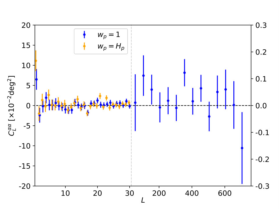 Figure 1
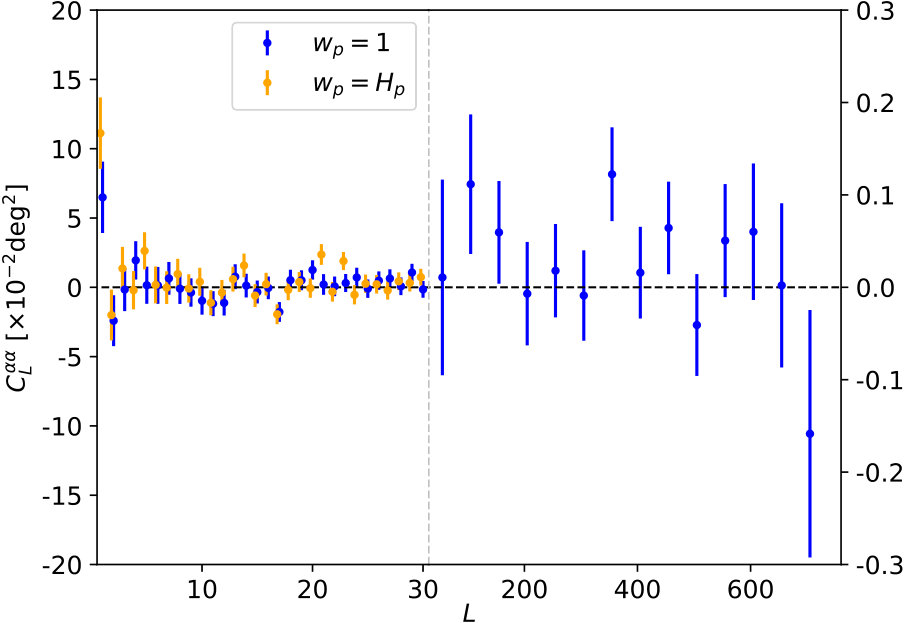 Figure 2
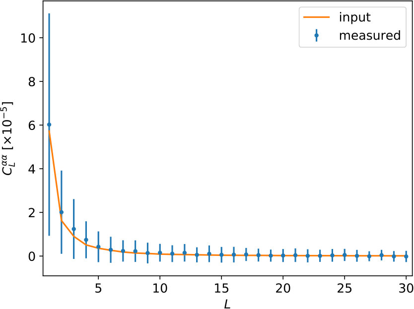 Figure 3
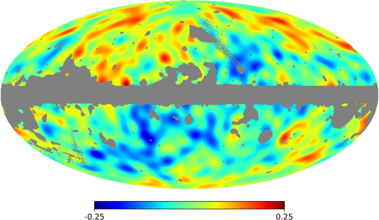 Figure 4
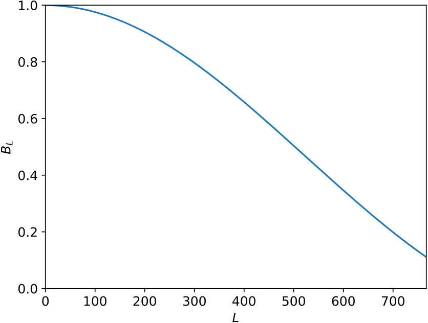 Figure 5
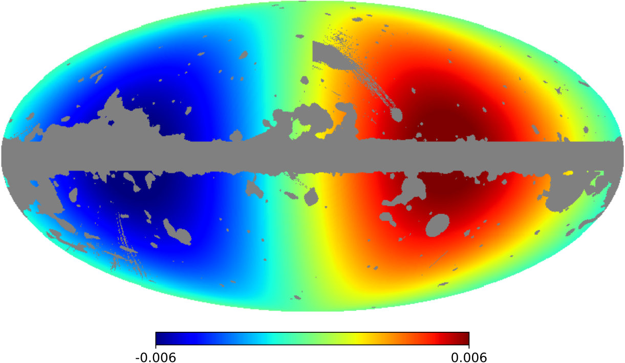 Figure 6
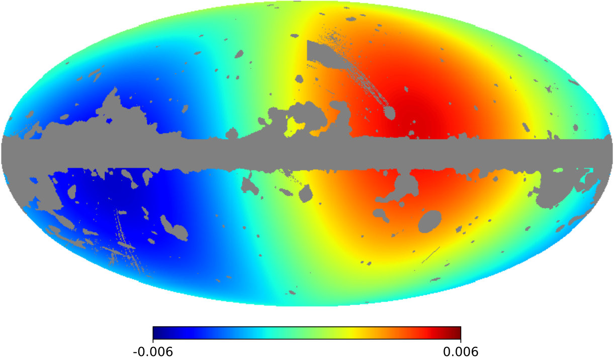 Figure 7
 Figure 8
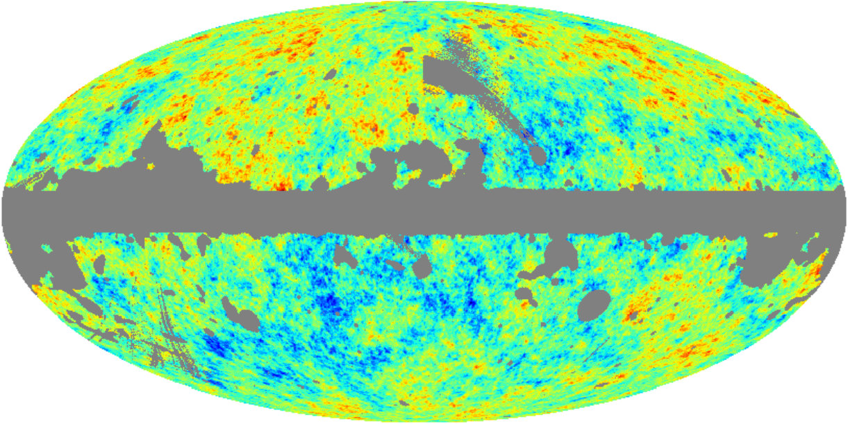 Figure 9
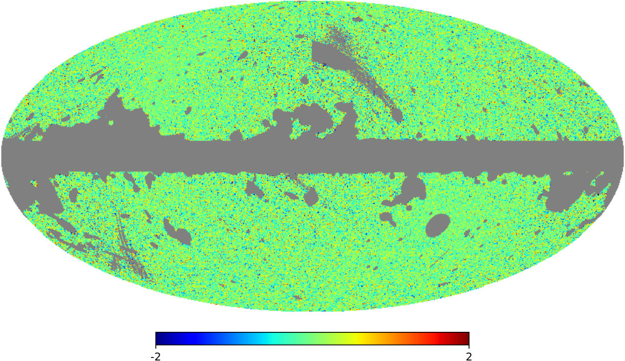 Figure 10
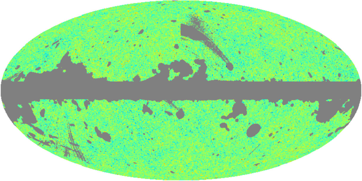 Figure 11
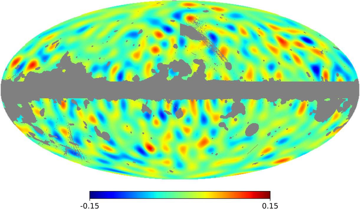 Figure 12
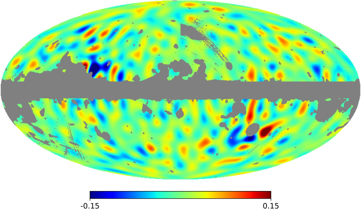 Figure 13
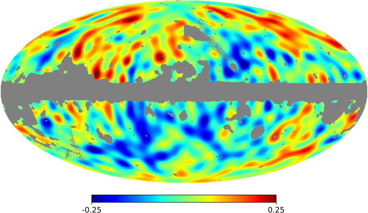 Figure 14
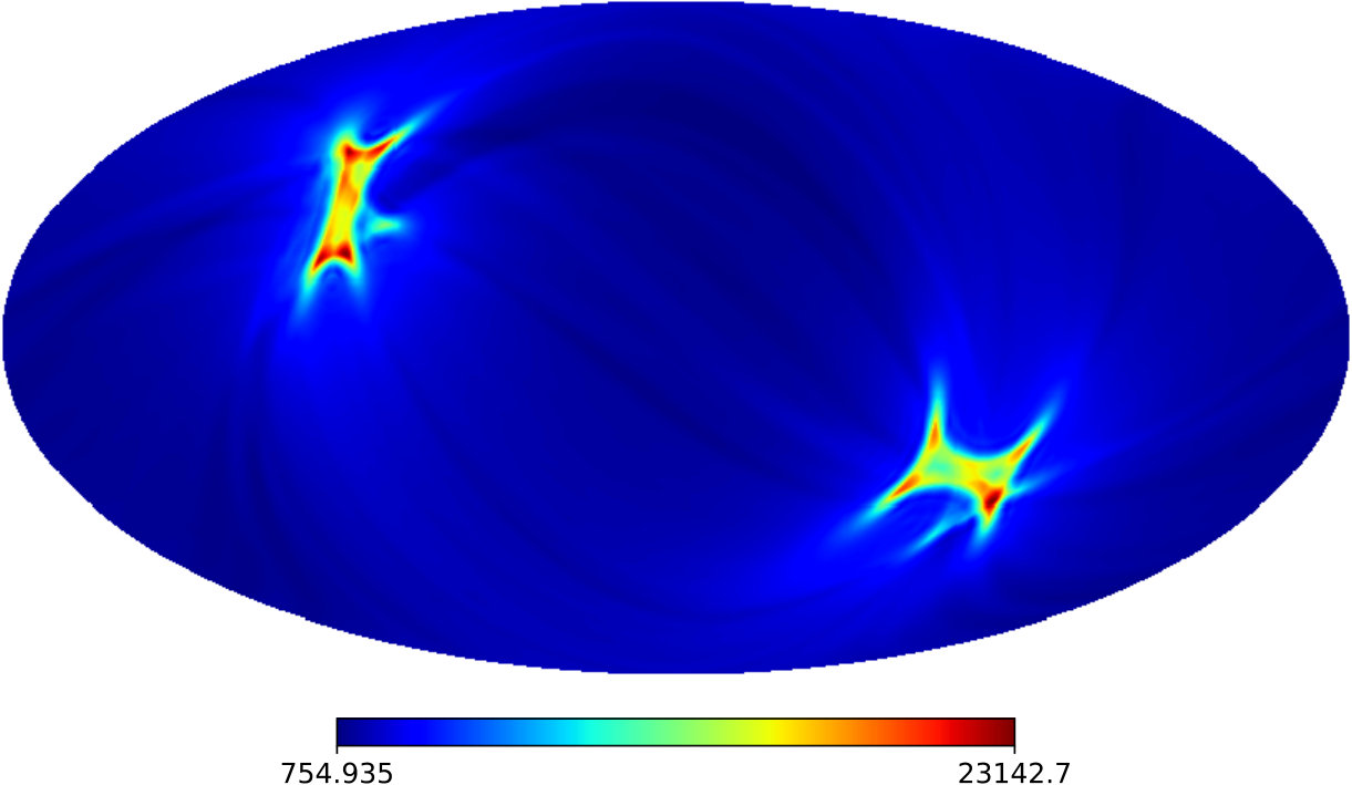 Figure 15
| Low | Low | All | BICEP2/Keck Array |
|---|---|---|---|
| Method | Amplitude | Direction |
|---|---|---|
| Uniform weighting | ||
| Hits-map weighting |
| Foreground | Low- PTE [%] | Dipole PTE [%] |
|---|---|---|
| Dust | 20.4 | 14 |
| Synchrotron | 20.0 | 97 |
| Free-free | 13.0 | 96 |
Peer Reviews
No public reviews on file for this paper yet. If you reviewed it on a platform where reviews are public (OpenReview, ICLR, NeurIPS, ICML), you can paste yours below so the community can read it here.
Videos
No videos yet. Explain this paper in a talk, walkthrough, or lecture? Add one.
Constraints on direction-dependent cosmic birefringence from
Planck polarization data
Dagoberto Contreras,11footnotetext: Corresponding author.
Paula Boubel
and Douglas Scott
Abstract
Cosmic birefringence is the process that rotates the plane of polarization by an amount, , as photons propagate through free space. Such an effect arises in parity-violating extensions to the electromagnetic sector, such as the Chern-Simons term common in axion models, quintessence models, or Lorentz-violating extensions to the standard model. Most studies consider the monopole of this rotation, but it is also possible for the effect to have spatial anisotropies. Paying particular attention to large scales, we implement a novel pixel-based method to extract the spherical harmonics for and a pseudo- method for . Our results are consistent with no detection and we set 95 % upper limits on the amplitude of a scale-invariant power spectrum of , on par with previous constraints. This implies specific limits on the dipole and quadrupole amplitudes to be \sqrt{C_{1}/4\pi}\lesssim 0\hbox{.!!^{\circ}}2 and \sqrt{C_{2}/4\pi}\lesssim 0\hbox{.!!^{\circ}}1, at 95 % CL, respectively, improving previous constraints by an order of magnitude. We further constrain a model independent quadrupole in an arbitrary direction to be \alpha_{20}=0\hbox{.!!^{\circ}}02\pm 0\hbox{.!!^{\circ}}21, with an unconstrained direction. However, we find an excess of dipolar power with an amplitude \sqrt{3C_{1}/4\pi}=0\hbox{.!!^{\circ}}32\pm 0\hbox{.!!^{\circ}}10\,(\mathrm{stat.})\,\pm 0\hbox{.!!^{\circ}}08\,(\mathrm{syst.}), in the direction , larger than 1.4 % of simulations with no birefringence. We attribute part of this signal to the contamination of residual foregrounds not accounted for in our simulations, although this should be further investigated.
1 Introduction
It is well known that our Universe violates parity via weak-sector interactions. It is natural then to look for violations of parity in other sectors. Here we use the cosmic microwave background (CMB) to constrain a Chern-Simons type parity violation in the electromagnetic sector [1]. In particular we focus on the effect of cosmic birefringence, which is the in vacuo rotation of the plane of polarization of photons. Such an effect would occur in modifications to electromagnetism or from higher-dimensional operators in effective field theories, such as the axion-photon coupling or in some quintessence models [2, 3], or in models with new scalar degrees that are not quintessence [4, 5, 6, 7, 8], or models driven by a modified gravitational interaction [9]. In these modifications, the addition of a term to the standard Lagrangian, which couples a new pseudo-scalar field (or vector field) to the electromagnetic term (or ), would affect left-handed photons and right-handed photons asymmetrically. This introduces a phase shift difference between orthogonal polarization states that would manifest itself as a rotation of the total linear polarization. A spatially-varying pseudo-scalar field would result in variations of this rotation angle, denoted by , across the sky. If such an effect were to exist, then it would be lost in any search for isotropic . Hence it is interesting to map out these potential fluctuations in .
A search for anisotropic birefringence is motivated because if, for example, the scalar field is dynamical, then it should have spatial fluctuations that would propagate as spatial variations in [6, 10, 8]. There are also models for which a uniform rotation vanishes, in which case these models would only be detectable in a search for the anisotropies of . If detected, the power spectrum of would give considerable insight on the nature of the source of birefringence and new physics. In particular the sourcing field could in principle contain a special direction (similar to birefringent crystals such as calcite or sapphire), which would impart a signal in a large scale map of . A final reason for such a study is a more practical one, namely that a uniform is degenerate with a systematic uncertainty in the orientation of the detectors, particularly polarization-sensitive-bolometers (PSBs) used in CMB experiments [11, 12]. Currently, measurements of a uniform rotation are systematics dominated at the |\alpha|\lesssim 0\hbox{.!!^{\circ}}3 level [13]. Searches for anisotropic can therefore in principle improve on this constraint, since a systematic uniform rotation would cancel out, along with the monopole in .
The CMB is particularly suited for measuring cosmic birefringence because it is polarized and because CMB photons propagate over cosmological distances essentially unimpeded, where such a rotation could accumulate into a detectable signal. CMB polarization is sourced by local density quadrupoles [14] at the surface of last scattering, producing linear - and -type polarization. These quantities can be decomposed by their geometric properties into - and -mode polarization components, which are the gradient (parity even) and curl (parity odd) modes of the polarization field on the sky [15, 16, 17]. Under the assumption of parity conservation the – and – correlations must be null, so that their measurement informs us of parity violations.
Cosmic birefringence has previously been constrained using CMB anisotropies from several experiments, most recently with Planck data, under the assumption of a uniform rotation. These results were found to be consistent with our expectation of no cosmic birefringence (see Ref. [13] and references therein). In this paper, we use the Planck 2015 (PR2) data to consider anisotropies in . While the possibility of an anisotropic has previously been addressed using data from other experiments [18, 19, 20, 21, 22, 23, 24], Planck data can provide more stringent constraints, particularly on the largest angular scales. Along with the power spectrum, we therefore constrain special directions in taking the form of a dipole or an quadrupole in an arbitrary coordinate system.
This paper is organized as follows. In Section 2 we explain the effect cosmic birefringence has on the CMB angular power spectra. In Section 3 we describe the data and simulations used. In Section 4 we describe our new map-space method used to estimate the angle locally as a function of direction on the sky. In Section 5 we demonstrate the effectiveness of our estimator on a known input signal. In Section 6 we present the results for our baseline analysis pipeline. In Section 7 we search for possible sources of systematic effects that might affect our results, and we finally conclude in Section 8.
2 Impact of birefringence on the CMB
A model of cosmic birefringence can be generated by including the following term in the electromagnetic Lagrangian:
[TABLE]
where is the electromagnetic field strength tensor and its dual, is a dimensionless coupling constant, is a suppressing mass (usually taken to be the Planck scale), and the potential depends on the details of the model. The symbol here denotes equality up to a total derivative that has no effect on dynamics. The interaction in Eq. (2.1) is exactly the form of the axion-photon coupling, while, for the symmetry suppresses couplings to other Standard Model particles [2]. The coupling of to treats left- and right-handed photons asymmetrically, leading to a rotation in the plane of polarization as photons propagate in vacuo. The amount of rotation is determined by the total change of the field along the photon travel path and is given by
[TABLE]
The existence of an angle that is non-zero would be reflected in the Stokes and polarization parameters, which would be modified as
[TABLE]
This effect induces – and – correlations that are otherwise expected to be zero, along with smaller modifications to the parity-conserving correlations. Specifically, the observed power (primed quantities) in these cross-correlations would be
[TABLE]
where the unprimed are the spectra that would be measured in the case of no cosmic birefringence. We will assume that is negligible, since Planck has no direct detection of modes. Employing the small-angle approximation222Our power spectrum results will demonstrate that this is a good approximation. In the event that this approximation breaks down, one should interpret the power spectrum to be for the quantity (as explained in Ref. [18]). (in ) we see that the only modifications to the CMB power spectra appear as non-zero and :
[TABLE]
where we have now allowed to depend on direction. As shown in Ref. [13], constraints on birefringence from Planck are driven by the – correlation, so we primarily focus on Eq. (2.11). This relation suggests that we can use local measurements of the – correlation to determine as a function of direction on the sky.
The correlations of Eqs. (2.4)–(2.9) can be searched for either in harmonic space or pixel space. In the spatial domain, one can look at the correlations between temperature extrema and polarization to reveal – cross-correlations. Similarly, correlations between -mode extrema and polarization reveal – correlations. Both approaches were used to constrain an isotropic in Ref. [13]. To analyse polarization data in the neighbourhood of extrema, or “peaks,” the modified Stokes parameters, and are used. This involves a transformation to radial and tangential components centred on each peak as the origin. Specifically, the value of at an angular distance from a peak is the radial ( 0) and tangential ( 0) component of the polarization with respect to the peak. The component is non-zero if the polarization is rotated by 45 with respect to these directions. The specific transformations are
[TABLE]
The transformed Stokes parameters are calculated in the neighbourhoods of each peak. The patterns are expected to have azimuthal symmetry, so the data can be compared to the following theoretical predictions (derived in Refs. [25, 13]):
[TABLE]
Here is a radial vector, with its magnitude, is a beam applied to the data, and is the pixel window function at HEALPix333http://www.healpix.sourceforge.net/ [26] resolution. The quantity is the second-order Bessel function of the first kind, and are bias parameters that arise from the selection of peaks from a Gaussian field [27, 28], which are discussed and calculated in Refs. [25, 13].
3 Data and simulations
Our baseline results use the full mission and half-mission Planck [29] data splits for the , , and polarization maps,444Available at http://www.cosmos.esa.int/web/planck/pla specifically using the SMICA component-separation procedure [30, 31], chosen for its relatively low noise level in polarization; however, we use Commander, NILC, and SEVEM maps to check for consistency. The maps are provided at a HEALPix resolution, smoothed with a beam. Along with these maps we use the common polarization mask UPB77 in union with a mask that covers missing pixels specific to the half-mission data split [31].555Though the areas affected by missing pixels are inadequate for measuring , they nevertheless have very little effect on our results. For our high-multipole likelihood (described in Section 4.2) we eventually degrade our maps to an resolution. We then define a new conservative mask that is simply the original mask degraded, with all pixels that contain a masked pixel in the original mask being set to zero.
It is worth recalling that in 2015 the Planck collaboration released polarization data with some known systematic effects still present. Specifically, there are large angular artefacts in the data that have yet to be remedied [29], temperature-to-polarization leakage effects at smaller scales [32, 33, 31], and a noise mismatch between the data and simulations [34]. We account for the large-scale artefacts by using high-pass-filtered versions of the data (and simulations), explicitly a cosine filter that nulls scales and transitions to unity at [31]. We note that the best-fit temperature-to-polarization leakage model was removed from the data [31] and had negligible effect on the uniform constraints [13], though we do not explicitly test for its impact here. The noise mismatch does not greatly affect our results, since our data come from the – cross-correlation; nevertheless we do use auto-correlations of (which are dominated by the – and – correlations [18]) on large scales in order to have a well defined likelihood (see Section 4.1) and have checked that results obtained are consistent with the cross-correlation of determined by the half-mission data.
We use a suite of simulations for which the power in is null, in order to estimate uncertainties for our power spectrum results. We generate polarization simulations using the following fiducial cosmology, which is consistent with the data [35]: ; ; ; ; ; ; ; and . Here are the physical densities. We add noise power to our simulations in order to match the total power in our data maps; this, however, does not include a correlated noise component or non-Gaussian foreground residuals. For our birefringence analysis the cosmological parameters are fixed to the values reported above. This seems to be a safe assumption, since has no effect on and only affects , and (and thus parameters) at second or higher order (see Eqs. 2.4–2.9). For small , the effect of lensing is orthogonal to an anisotropic birefringence [18, 36], however a bias appears at the power spectrum level [37]. This bias on the power spectrum is, however, sub-percent at Planck noise levels [37] and therefore we ignore its effects here. We further generate a suite of simulations with a particular scale-invariant power spectrum, described in Section 5, to demonstrate the effectiveness of our reconstruction and to determine the corresponding reconstruction bias.
4 Measuring locally
We use Eq. (2.15) to define an unbiased estimator for at the location of every peak ():
[TABLE]
Here is the value of the data, and is a radial vector centred at the location of peak . The peak positions are determined by the full-mission -mode map, while the above fit is performed on the full or half-mission and maps. Equation (4.2) is a simple linear least-squares fit to with the identity as the covariance matrix for and the sum is performed over all unmasked pixels within a radius (chosen since the profile vanishes at distances >1\hbox{.!!^{\circ}}5, as demonstrated in Refs. [25, 38, 13]). We also remove the monopole in , to suppress any leakage to higher multipoles, since the monopole is systematics dominated and large [13]; however, we check that this step has no significant effect on our results.
We fit for a scale-invariant power spectrum, which takes the form
[TABLE]
for a constant . By convention we refer to multipoles as “” to distinguish them from multipoles (for the temperature and polarization anisotropies). This spectrum would be realized in a model containing nearly massless psuedo-scalar degrees of freedom coupled to photons, such as in Ref. [8], for . A model like this is constrained extremely well at low compared to high , which puts Planck data at a distinct advantage compared to smaller coverage (although with higher sensitivity) ground-based experiments. For this reason we pay particular attention to recovering the low s accurately (see Section 4.1).
Previous estimators of anisotropic in the literature compute the contribution to the 4-point function (of or ) in harmonic space using standard quadratic maximum likelihood techniques [18] (similar to CMB lensing techniques), or using the 2-point correlation function [20, 21]. Our approach reconstructs the 4-point function by simply measuring the variation of the 2-point function locally in the data. In the following subsections we describe how we take the local measurements of and compute maps at low and high resolution. For power spectra it is worth recalling that the auto-spectra of an -map determined by the – correlation is not the power spectrum of . This is because the auto-spectrum necessarily contains contributions from the – and – correlations that are non-zero even if [18]. One can obtain the true power spectrum by subtracting the mean power spectrum from simulations with a null spectrum or by using cross-correlations; we employ both of these methods below.
4.1 Low multipoles
We begin by taking the values found above and using a pixel fit to recover the spherical harmonics ,
[TABLE]
Here the weights are uniform per pixel or chosen to incorporate the uneven hits distribution from the Planck scanning strategy. For our baseline we use a uniform weighting scheme ; however, we also consider a weighting scheme where is given by a smoothed version of the 217-GHz hits map666The map is smoothed with a top-hat beam, chosen to match our method of Section 4 that fits for over pixels within of each peak. (denoted , which we plot later). Note that our simulations do not contain the effects of the Planck scan strategy and therefore only uniform weighting is used for them. This method accounts for the mask by simply not using any masked pixels, i.e., all values come from unmasked areas. We then compute the power spectrum of either by taking the cross-correlation of and , determined with the half-mission 1 and 2 maps, or by taking the auto-spectrum of determined by the full-mission data and subtracting the mean of the auto-spectra calculated from null simulations. The latter method is in principle more sensitive to the noise properties of the data, but we find it to be consistent with the former method, and it has the advantage of allowing us to form a Gaussian likelihood for the s when fitting for a model. For this reason we only display these auto-correlation spectra in our low results that follow.
A direct calculation of Eq. (4.4) is computationally expensive for large , so we limit this approach to and consider higher multipoles only in the following subsection. The low- likelihood then takes the form
[TABLE]
The average is taken over a suite of simulations with . is a normalizing factor to ensure that our estimator is unbiased, and is determined by cross-correlating the input realizations with their corresponding measured value from a reference power spectrum. Bayes’ theorem, along with a flat prior on (specifying ), allows us to turn this into a likelihood for given the data and hence to obtain the posterior for the amplitude of a scale-invariant spectrum.
4.2 High multipoles
To produce our high- map we need to apply a smoothing to our values. The mean separation between peaks is about 0\hbox{.!!^{\circ}}2, and therefore we define an map (denoted ) populated with the mean of over all pixels within a radius of 0\hbox{.!!^{\circ}}25:
[TABLE]
This procedure induces a beam function (), which we show in Fig. 1. Our high- power spectrum is the cross-correlation of Eq. (4.7) between half-mission 1 and half-mission 2 data, with a correction for the beam and the cut sky, i.e.,
[TABLE]
where is the fraction of the unmasked sky, is the applied mask, is the effective beam function (see Fig. 1) induced by the smoothing procedure, and is the pixel window function specific to an resolution map. The approximation in Eq. (4.9) is the exact MASTER [39] correction due to the masking for an -independent power spectrum for which the data and simulations are consistent. We further bin the power spectrum in bins of size (with so as not to double count the low- data), to minimize correlations induced by the mask from neighbouring modes.
To fit for a scale-invariant power spectrum (Eq. 4.3) we form as a function of :
[TABLE]
where is the binned inverse covariance matrix derived from simulations (generated with ) and is the model power spectrum (Eq. 4.3) binned in the same way as the data and simulations. We have verified with our simulations that each bin is close to Gaussian and so we form a likelihood as
[TABLE]
Once again we can transform this into a likelihood for given the data, with a flat prior on .
Finally we combine our low- and high- likelihoods to form a joint constraint on by simply taking the product of the likelihoods in Eqs. (4.6) and (4.11). This assumes that the data at low are uncorrelated with the data at high . This is known to not be strictly true, since the mask will induce correlations, particularly for with the first bin of the high- data (which uses ). However, this small correlation has very little impact on our results and the difference in the results is minimal if is increased to reduce the correlation.
5 Tests of the method
We first test the method described above in Section 4 by generating a single simulation with a known realization of from an input power spectrum. To do this we generate a and realization from the cosmology described in Section 3, and we then modify the and maps by the relation Eq. (2.3). In this test the map is a realization of a scale-invariant power spectrum with (chosen for visualization purposes), and is shown in Fig. 2 (left panels). We further input a noise realization to our simulation, so that the total power in each of the and maps is consistent with the data.
Upon applying our method of recovering , we obtain the panels on the right-hand side of Fig. 2, for both low and high resolution. At the level of the maps the output of our analysis is quite consistent with the input; however, there is considerably more noise in our output maps (particularly at high resolution) due to the addition of significant noise power. At the power spectrum level we also obtain very good agreement with our input spectrum, with the scatter attributable to the noise in the simulation. In Fig. 3 we show the mean recovered power spectrum on a suite of simulations with , along with the theoretical curve and the corresponding uncertainties. We find that our reconstruction slightly overestimates the true power spectrum at the 30 % level, which we correct for in the parameter in Eq. (4.6).
6 Results
First we confirm that we recover the results for the -monopole from Ref. [13]. However, as already noted, in the main analysis of this paper we remove the monopole (which is dominated by systematic effects) so that it does not leak into higher multipoles.
6.1 Maps and power spectrum
Our low- and high- maps for the data are shown in the top row and bottom right panels of Fig. 4, respectively. Our two low- maps are clearly strongly correlated; however, using the weighting given by the hits map in Fig. 4 (bottom left) we see large-scale features near the Ecliptic poles and Galactic plane. While, visually striking, these features appear to have very little effect on our power spectrum results (to be discussed in Section 7.1). They nevertheless point to systematic effects associated with residual foregrounds not accounted for in our simulations.
The power spectrum at low and at high (binned) are shown together in the left panel of Fig. 5. Recall that at low the spectrum is the mean of the auto-spectrum of our simulations subtracted from the auto-spectrum of our low- -map. We find that this estimate is consistent with the cross-correlation of from half-mission 1 and half-mission 2 data. The blue points in this figure use the uniform weighting scheme, while the orange points use the hits-map weighting. At high the spectrum is derived using cross-correlations only. We find good agreement with the expectation of a null power spectrum over all (with the possible exception of the mode, the discussion of which is left for Section 6.3), and the smallness of the power spectrum justifies our use of the small-angle approximation in Eq. (2.11).
6.2 Constraints on a scale-invariant power spectrum
The posterior for the amplitude of a scale-invariant power spectrum is shown in Fig. 5 (right). The high- likelihood prefers a positive at less than the level, while the low- data are consistent with . However, they are both quite consistent with each other, as can be seen by comparing the 95 % CL values for the low- likelihoods and the full likelihood in Table 1. The full- constraint comes from the combination of the low- and high- likelihoods, assuming no correlation between the two. Due to the dependence of the model spectrum, the likelihood is dominated by the lowest s (a bluer spectrum would be more constrained by high than the scale-invariant one). Note that the posterior is not very Gaussian, since the s follow a distribution. We find the constraint at 95 % CL. This constraint is at a similar level to the systematic uncertainty of the -monopole measurements, namely 0\hbox{.!!^{\circ}}3. This suggests that, in the absence of an improved absolute calibration scheme (see Ref. [40], for an example of efforts in this direction), constraints on cosmic birefringence from the next generation of CMB measurements will likely be focused on searches for anisotropic .
While the noise level of Planck polarization data is large compared to the most recent ground-based experiments, it does have the distinct advantage of measuring the largest scales. Our new constraints improve upon the most stringent constraints available (see Table 1) and are an order magnitude smaller than previous results [18, 23]. Somewhat tighter constraints could be found using a joint low- and high- analysis of data from Planck combined with the BICEP2/Keck Array.
The difference between our low- likelihoods using two different weighting schemes is attributable to residual foregrounds (explored in Section 7.1) that are not accounted for in our simulations. The hits-map weighting is more sensitive to these foregrounds compared to the uniform weighting. In Section 7.1 we derive a systematic error for our amplitude, which primarily comes from residual polarized dust.
6.3 The dipole
From the power spectrum, Fig. 5 (left panel), we see that the dipole deviates the most from the expectation of a null power spectrum. We quantify this by comparing for the data to the values in our simulations. We find that only about 1.4 % of the simulations have a larger dipole than the data.777For these results we include obtained by our – estimator as well, although this has only a marginal influence on our results. This is the case for both the auto-correlation and cross-correlation of the full-mission or half-mission data sets. It is therefore worth investigating this signal further.
In the absence of a model, the values of are Gaussian distributed with mean zero and variance given by , where the average is taken over simulations with a null dipole. We can convert this to an amplitude and direction with a uniform prior on the s, parameterizing the dipole as
[TABLE]
Here is defined as the angle with respect to the best-fit direction and . In Table 2 we quote the mean values of the posteriors and their corresponding 68 % uncertainties. We show the best-fit dipoles in Fig. 6 for our baseline results (right panel) and using hits-map weighting (left panel). We explore in Section 7.1 the effect of residual foregrounds (not present in our simulations) on the dipole and find that these significantly affect the direction of the dipole.
If the dipole in were to be physical (and not simply a statistical fluctuation), then the overall signal could be fit by a sufficiently red spectrum, which would have significant implications on the nature of the sourcing pseudo-scalar (or vector) field. Alternatively, there could be a genuinely preferred direction for the cosmic birefringence (i.e., a dipole that is unconnected to a power spectrum). Either way, new (preferably) all-sky polarization data with reduced noise levels compared to Planck are required to determine whether or not the dipole signal is cosmological.
6.4 The quadrupole
While there is no evidence for a significantly large quadrupole in the data (see Fig. 5, left), there could be a special direction in the map that would show up solely in the mode. It is therefore worth considering this mode specifically.
An quadrupole in an arbitrary direction would be related to our coordinate values by a rotation with a Wigner -matrix by
[TABLE]
Here is an quadrupole in a coordinate system pointing in the direction . With our simulations we generate a covariance, from our simulations, which defines a likelihood of the form
[TABLE]
We then sample the likelihood using a Markov chain Monte Carlo (MCMC) algorithm to obtain posteriors for the parameters , , and . Marginalizing over the direction we find \alpha^{\prime}_{20}=0\hbox{.!!^{\circ}}02\pm 0\hbox{.!!^{\circ}}21, which is very consistent with no special direction in the quadrupole. For this same reason the direction is unconstrained.
7 Systematic effects
In Section 3 we mentioned several kinds of systematic effect that are present in the Planck polarization data that we have taken efforts to avoid being sensitive to. These are: an uncertainty in the global orientation of the PSBs; large-scale artefacts in the data; and an un-modelled correlated noise component in the data. The first effect contributes a bias to a uniform and would thus cancel out in our search for anisotropic . The second is mitigated by the use of high-pass-filtered data. The last effect is minimized by using cross-correlations (between half-mission 1 and half-mission 2 data) wherever possible. Our low- likelihood uses auto-correlations, although we compared our power spectra to the corresponding cross-correlation and found good consistency. However, this does not definitively show that correlated noise is not a significant bias for our results, and so we now further investigate other potential sources of systematic effects.
7.1 Foregrounds
Our estimator looks for parity violations in the CMB data in the hopes of constraining a cosmological signal. Foregrounds contaminate this by being large additive signals that do not source polarization in a way that is invariant under parity transformations about our location, and hence can corrupt the signature.
We first test for this contamination by enlarging our baseline mask to cover more of the Galactic plane. We take the UPB77 mask [31], smoothed with a beam, then set all points below 0.9 to zero and all others to 1, and finally multiply by the UPB77 mask again so as not to miss any small masked areas. This decreases the sky fraction available from UPB77 from to 0.69. This roughly 10 % decrease in sky coverage leads to a roughly 40 % increase in the 95 % CL in the amplitude of a scale-invariant power spectrum, due to increased sample variance. Since the likelihood is dominated by low and is skewed to higher values (see Fig. 5, right panel), this result is still quite consistent with our baseline result. However, we cannot entirely rule out that foregrounds might be a significant systematic effect here. With that in mind, it is nevertheless still the case that the increase in the 95 % CL limit is consistent with no detection of anisotropic .
As an additional test we can define an a posteriori mask to be zero everywhere that the absolute value of the low- map in Fig. 4 (top left) is greater than 0.15, masking the visually striking features. We find that our power spectrum results remain consistent with the expectation of the corresponding increased sample variance. In particular the dipole is consistent in amplitude and direction with our baseline results from Table 2.
Some foreground contaminants, such as dust, can produce modes that might induce a cross-correlation signal between lensing and . We test for this using the Planck 2015 lensing maps [41] and perform the cross-correlation with our low- data and simulations. Note that the Planck lensing maps contain no information for [41], so this test tells us nothing about the nature of the dipole in . Nevertheless, we obtain a probability to exceed (PTE) the obtained with the data (derived from simulations), of 25 %, consistent with no detection of a cross-correlation.
We also test for the presence of correlated polarized synchrotron, free-free, and dust emission directly, by obtaining the Planck , and foreground maps [30] and propagating them through our analysis to obtain maps of (denoted ). That is, we use Eq. (4.2) to fit for in the foreground maps at the location of peaks in the CMB -mode map. These maps contain an unnormalized estimate of the contribution from each foreground to that is correlated with the CMB. We then determine a PTE for the obtained with the cross-correlation of with , shown in Table 3. We find marginally significant correlations with dust only. In order to estimate the bias incurred from these foregrounds we model the contamination as
[TABLE]
Here are the measured data, while are the expected data coming just from the CMB, is the cross-correlation of obtained from the CMB and foreground, and is the auto-correlation of obtained from the foreground (with these quantities being estimated from the data). Propagating to obtain 95 % CL values for the scale-invariant amplitude leads to a decrease of 0.7 (still consistent with no detection). Note that this is the same amount of shift between our low- likelihoods using hits-map weighting compared to uniform weighting; we thus assign this value as a systematic error in our result, present because our simulations do not contain residual foregrounds. When applied to the mode specifically, we find that the dipole moves away from the Galactic plane by the same amount as the difference between the hits-map weighted and uniform weighted dipole (see Table 2), consistent with the presence of residual correlated foregrounds; however, the amplitude remains largely unchanged. We therefore assign a conservative systematic error of 0\hbox{.!!^{\circ}}08 to the amplitude and to the direction, substantially impacting its significance.
7.2 Point sources
Although point sources in general add a source of bias to the 4-point function [42], they are not expected to contaminate the signal we are looking for [18], since they only contribute a parity-even signal. Nevertheless we test the level of contamination by including a point-source mask.
We consider the union of the Planck point source masks for polarization from 100 to 353 GHz. It turns out the vast majority of pixels masked by the point source mask are already masked by UPB77. After degrading to a common resolution of , there are 16 remaining pixels (out of a potential 24,000) that are not also masked by UPB77. It should come as no surprise then that they therefore have a negligible effect on our results and we thus consider point sources to be an unimportant systematic for our analysis.
7.3 Relative uncertainty on the PSB orientations
Although we are insensitive to a global rotation of the HFI detectors, we could still in principle be sensitive to a relative angular separation between individual PSBs. This is because, in the component separation process, different frequencies (and thus PSBs) are used anisotropically, and thus a relative difference in orientation of PSBs at different frequencies would appear as anisotropic birefringence.
The relative upper limit on the PSB orientations is 0\hbox{.!!^{\circ}}9 [43], however the dispersion of , as measured using – correlations between the HFI frequencies, is around 0\hbox{.!!^{\circ}}2 [44]. We expect that such an anisotropy would appear as a large-scale feature characterizing the use of different frequencies in the component-separation process. Thus we do not expect that this would affect the search for a scale-invariant spectrum. Crudely speaking the use of different frequencies varies mostly with latitude (though this depends upon the method [31]), which is a pattern we do not see. In particular the dipole is seen mainly in the Galactic plane, as opposed to the Galactic poles. Therefore it seems unlikely that the excess in the dipole we see is due to the relative uncertainty in PSB orientations compared to foregrounds; however, a full characterization of such effects will be important for future studies.
8 Conclusions
We have estimated the anisotropy in the cosmological birefringence angle, , with a novel map-space based method, using Planck 2015 polarization data. Our results are consistent with no evidence for parity-violating physics. We provide the most stringent constraints on the anisotropy at large angular scales and have constrained a scale-invariant amplitude to be at 95 % CL.888Conservatively, one should take the full 95 % limit to be . Here the systematic error comes from estimating residual foregrounds (primarily dust) in the data. This implies a constraint on dipolar and quadrupolar amplitudes to be \sqrt{C_{1}/4\pi}\lesssim 0\hbox{.!!^{\circ}}2 and \sqrt{C_{2}/4\pi}\lesssim 0\hbox{.!!^{\circ}}1, respectively. These constraints are, along with the newest results from the BICEP2/Keck Array, the tightest limits on a scale-invariant power spectrum (see Table 1 for a direct comparison). We also search for special directions in , finding that an quadrupole is constrained to be \alpha_{20}=0\hbox{.!!^{\circ}}02\pm 0\hbox{.!!^{\circ}}21, consistent with the null hypothesis. Our results are consistent across four different component-separation methods and do not appear to be significantly contaminated by point sources. We also find no significant cross-correlation signal between our maps and the Planck 2015 lensing map.
One possible exception to the above conclusion is the dipole in (whose best-fit amplitude and direction can be found in Table 2, corresponding to a radial 68 % uncertainty on the direction of ), which is somewhat large compared to null simulations, with an associated p-value of 1.4 %. We find that the significance is insensitive to the use of the auto-correlation of full-mission data or the cross-correlation of the half-mission data. We do find that foreground contamination, coming primarily from dust, biases the dipole in a significant way, pulling the direction toward the Galactic plane, accounting for part of the signal. If, on the other hand, some of the dipole is genuinely due to cosmic birefringence then this would have significant implications for the form of the field and the source of its fluctuations, necessitating a red spectrum or a specifically direction-dependent birefringence. The model-space is vast and the significance is low, and clearly partially contaminated by residual foregrounds, so we do not speculate on what the physical source could be here. More sensitive polarization data at large angular scales are required to settle the issue.
In Ref. [13] it was determined that searches for a uniform angle are now dominated by systematic effects at the 0\hbox{.!!^{\circ}}3 level. Here we find that constraints on the direction dependence of are also at about the 0\hbox{.!!^{\circ}}3 level, with no apparent dominant systematic effects limiting the search in the near future. Therefore in the absence of an improved calibration scheme for determining the orientation of the PSBs, future searches for parity-violating physics of the form discussed here will likely be driven by the pursuit of for anisotropic cosmic birefringence.
Acknowledgments
This work was supported by the Natural Sciences and Engineering Research Council of Canada (NSERC).
The reference list from the paper itself. Each links out to its DOI / PubMed record.
- 1[1] S. M. Carroll, G. B. Field and R. Jackiw, Limits on a Lorentz and Parity Violating Modification of Electrodynamics , Phys. Rev. D 41 (1990) 1231 . · doi ↗
- 2[2] S. M. Carroll, Quintessence and the rest of the world , Phys. Rev. Lett. 81 (1998) 3067–3070 , [ astro-ph/9806099 ]. · doi ↗
- 3[3] A. Lue, L.-M. Wang and M. Kamionkowski, Cosmological signature of new parity violating interactions , Phys. Rev. Lett. 83 (1999) 1506–1509 , [ astro-ph/9812088 ]. · doi ↗
- 4[4] J.-Q. Xia, Cosmological CPT Violation and CMB Polarization Measurements , JCAP 1201 (2012) 046 , [ 1201.4457 ]. · doi ↗
- 5[5] M. Li, Y.-F. Cai, X. Wang and X. Zhang, C P T 𝐶 𝑃 𝑇 CPT Violating Electrodynamics and Chern-Simons Modified Gravity , Phys. Lett. B 680 (2009) 118–124 , [ 0907.5159 ]. · doi ↗
- 6[6] M. Pospelov, A. Ritz, C. Skordis, A. Ritz and C. Skordis, Pseudoscalar perturbations and polarization of the cosmic microwave background , Phys. Rev. Lett. 103 (2009) 051302 , [ 0808.0673 ]. · doi ↗
- 7[7] F. Finelli and M. Galaverni, Rotation of Linear Polarization Plane and Circular Polarization from Cosmological Pseudo-Scalar Fields , Phys. Rev. D 79 (2009) 063002 , [ 0802.4210 ]. · doi ↗
- 8[8] R. R. Caldwell, V. Gluscevic and M. Kamionkowski, Cross-Correlation of Cosmological Birefringence with CMB Temperature , Phys. Rev. D 84 (2011) 043504 , [ 1104.1634 ]. · doi ↗