The clustering of the SDSS-IV extended Baryon Oscillation Spectroscopic Survey DR14 quasar sample: First measurement of Baryon Acoustic Oscillations between redshift 0.8 and 2.2
Metin Ata, Falk Baumgarten, Julian Bautista, Florian Beutler, Dmitry, Bizyaev, Michael R. Blanton, Jonathan A. Blazek, Adam S. Bolton, Jonathan, Brinkmann, Joel R. Brownstein, Etienne Burtin, Chia-Hsun Chuang, Johan, Comparat, Kyle S. Dawson, Axel de la Macorra, Wei Du

TL;DR
This paper measures the BAO scale using quasars from eBOSS between redshifts 0.8 and 2.2, providing the first such measurement in this redshift range and confirming consistency with Planck cosmology.
Contribution
First measurement of BAO feature between redshifts 1 and 2 using quasar clustering, enhancing the cosmological distance ladder and testing ΛCDM model.
Findings
BAO detected at >2.8σ significance in quasar clustering
BAO distance at z=1.52 measured with 3.8% precision
Results consistent with Planck ΛCDM predictions
Abstract
We present measurements of the Baryon Acoustic Oscillation (BAO) scale in redshift-space using the clustering of quasars. We consider a sample of 147,000 quasars from the extended Baryon Oscillation Spectroscopic Survey (eBOSS) distributed over 2044 square degrees with redshifts and measure their spherically-averaged clustering in both configuration and Fourier space. Our observational dataset and the 1400 simulated realizations of the dataset allow us to detect a preference for BAO that is greater than 2.8. We determine the spherically averaged BAO distance to to 3.8 per cent precision: Mpc. This is the first time the location of the BAO feature has been measured between redshifts 1 and 2. Our result is fully consistent with the prediction obtained by extrapolating the Planck flat…
Click any figure to enlarge with its caption.
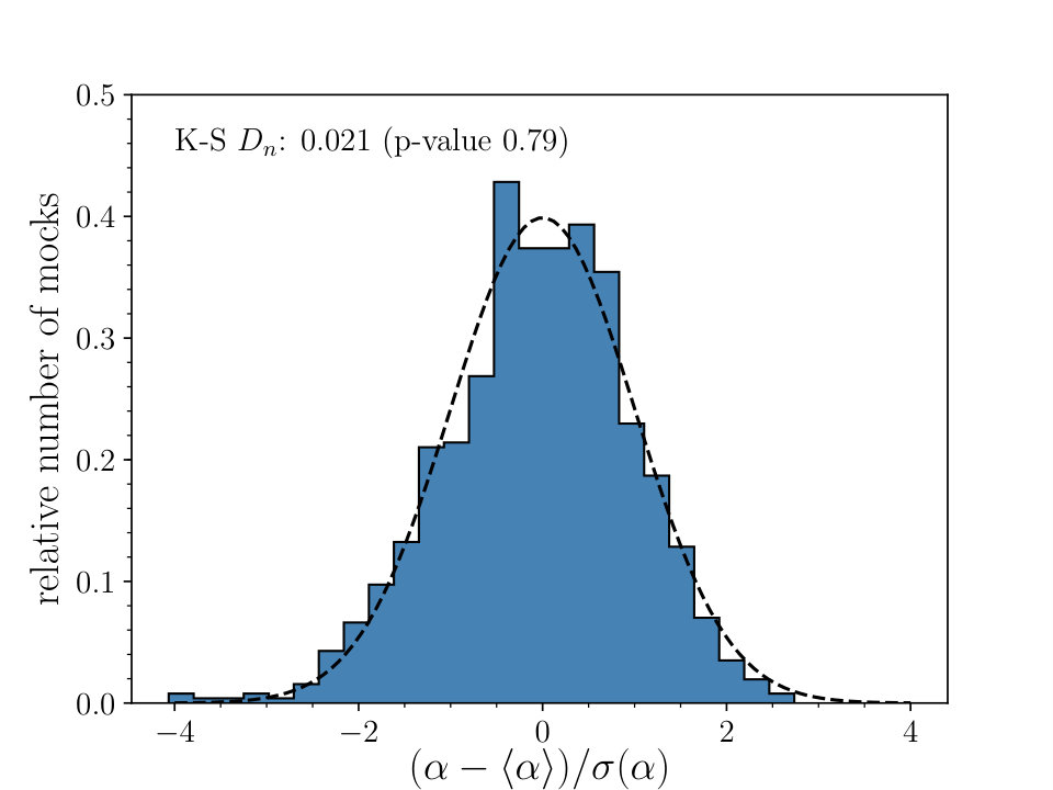 Figure 1
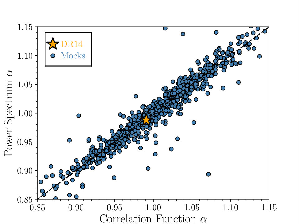 Figure 2
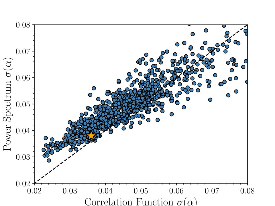 Figure 3
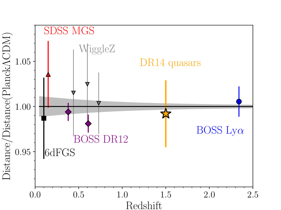 Figure 4
 Figure 5
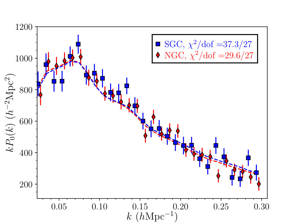 Figure 6
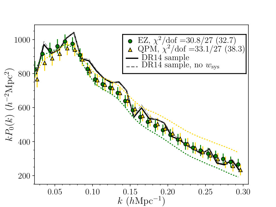 Figure 7
 Figure 8
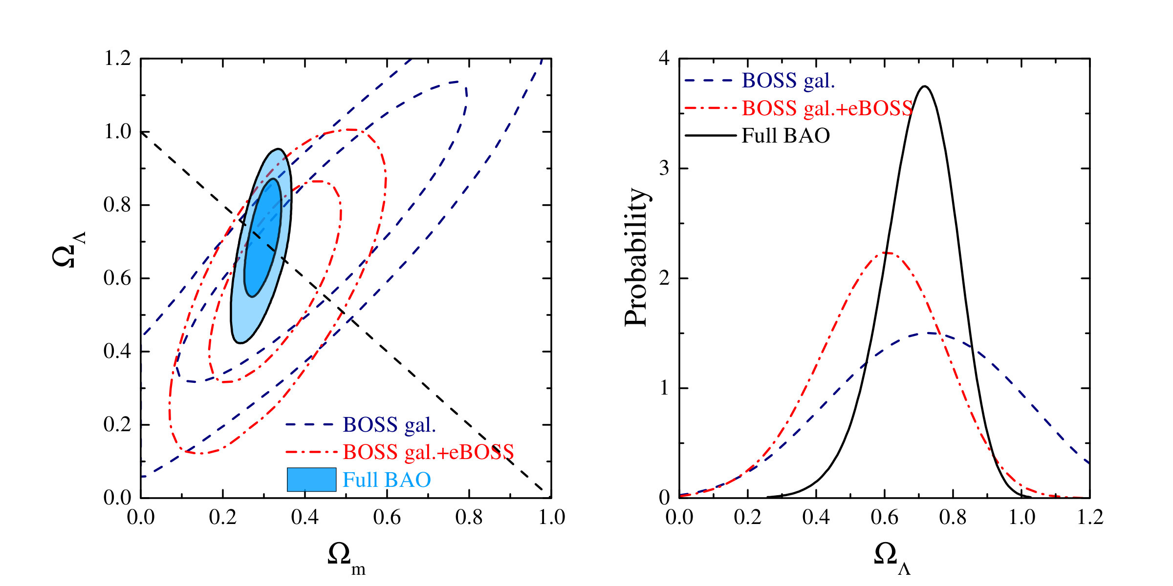 Figure 9
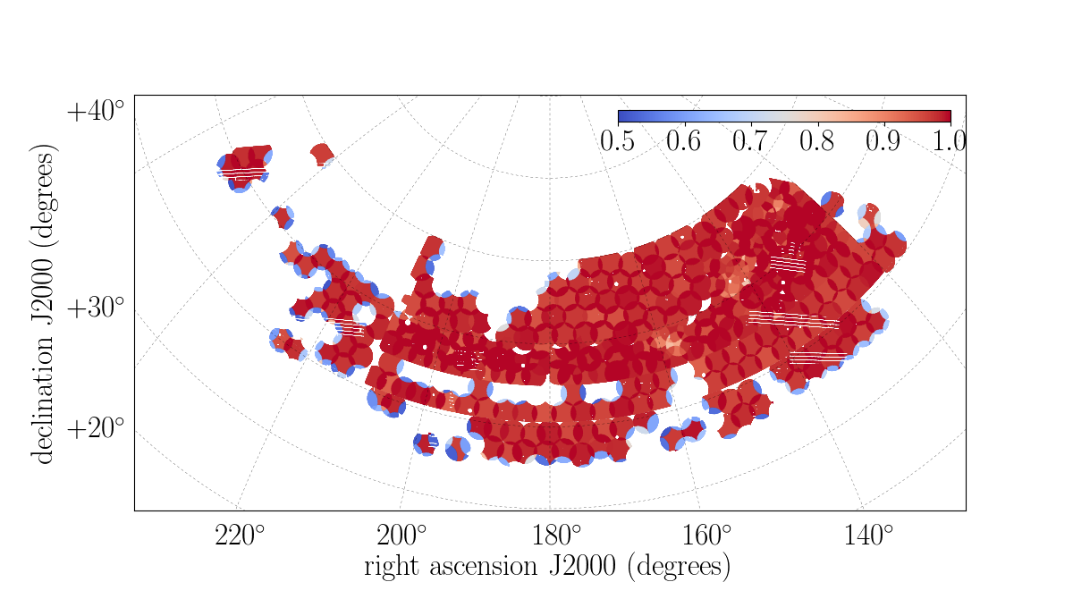 Figure 10
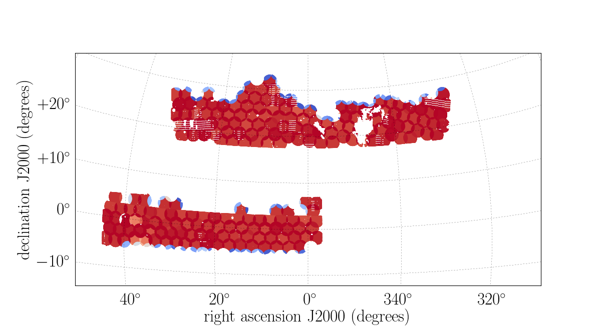 Figure 11
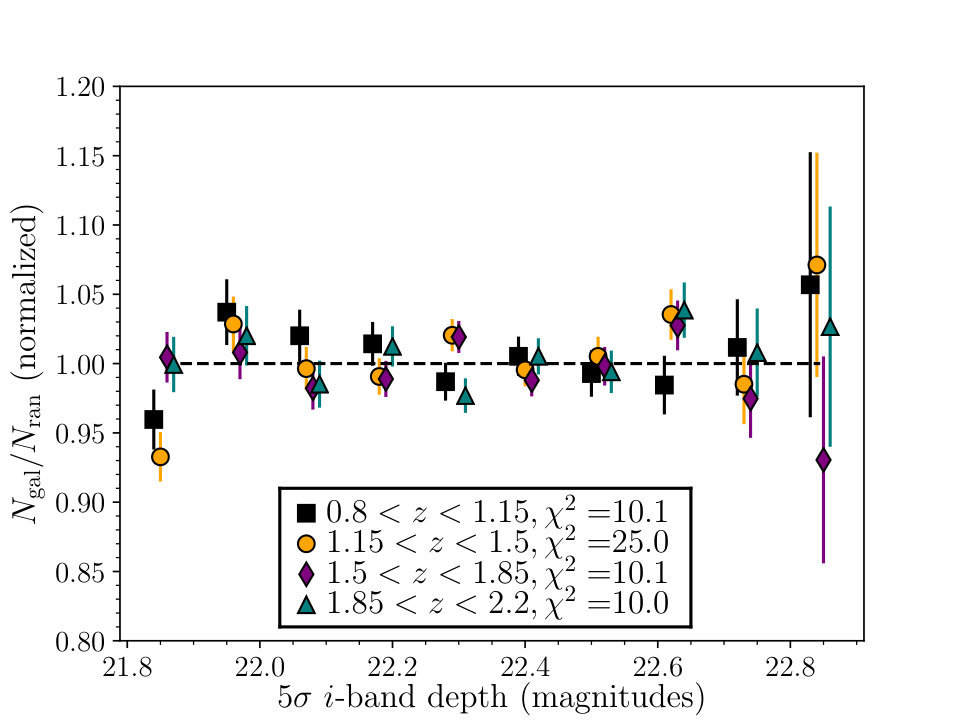 Figure 12
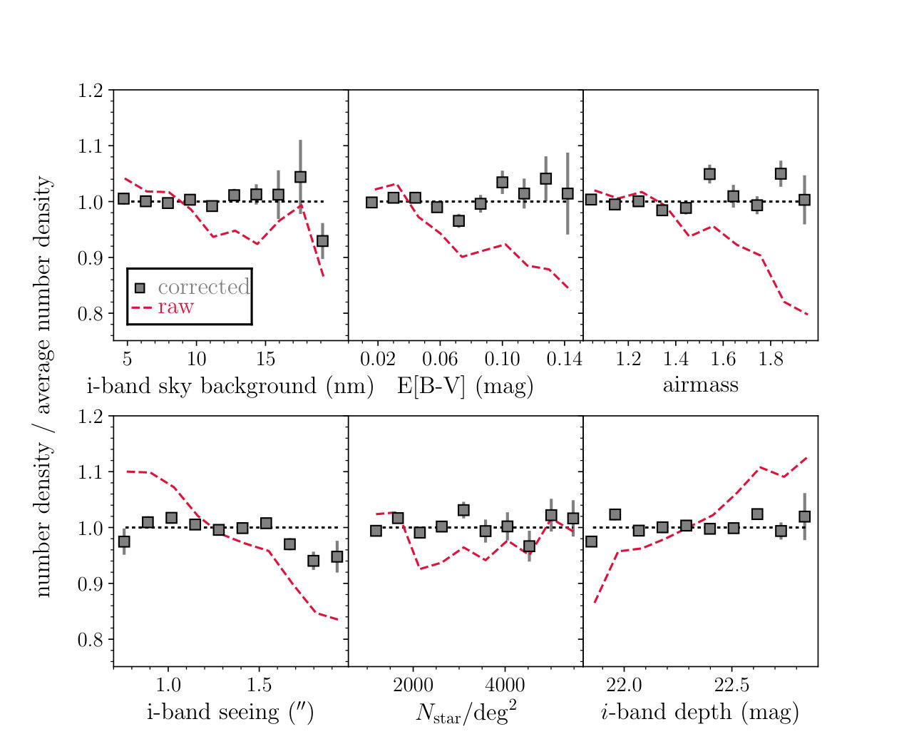 Figure 13
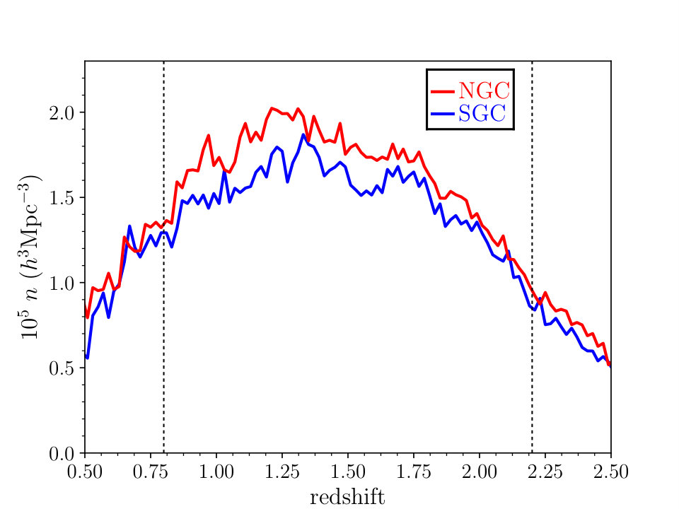 Figure 14
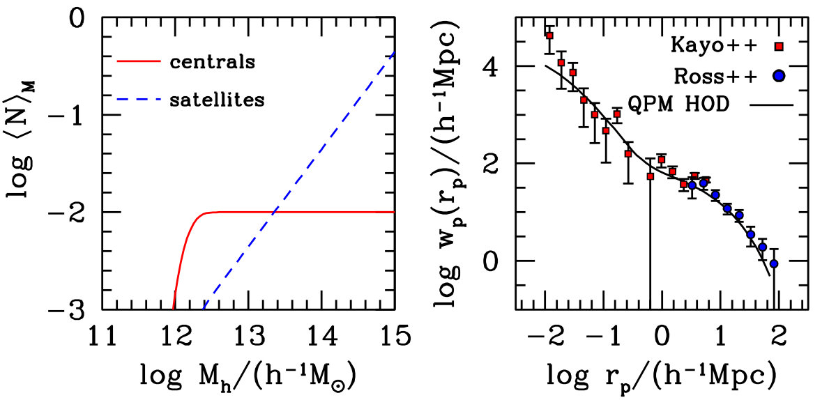 Figure 15
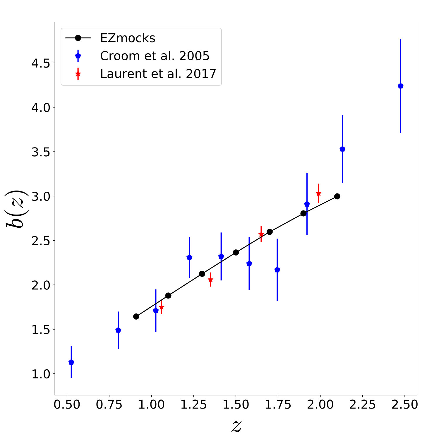 Figure 16
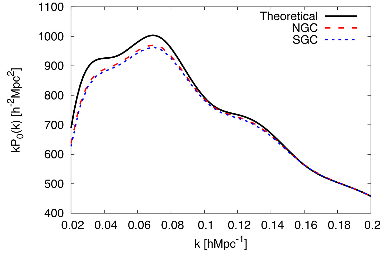 Figure 17
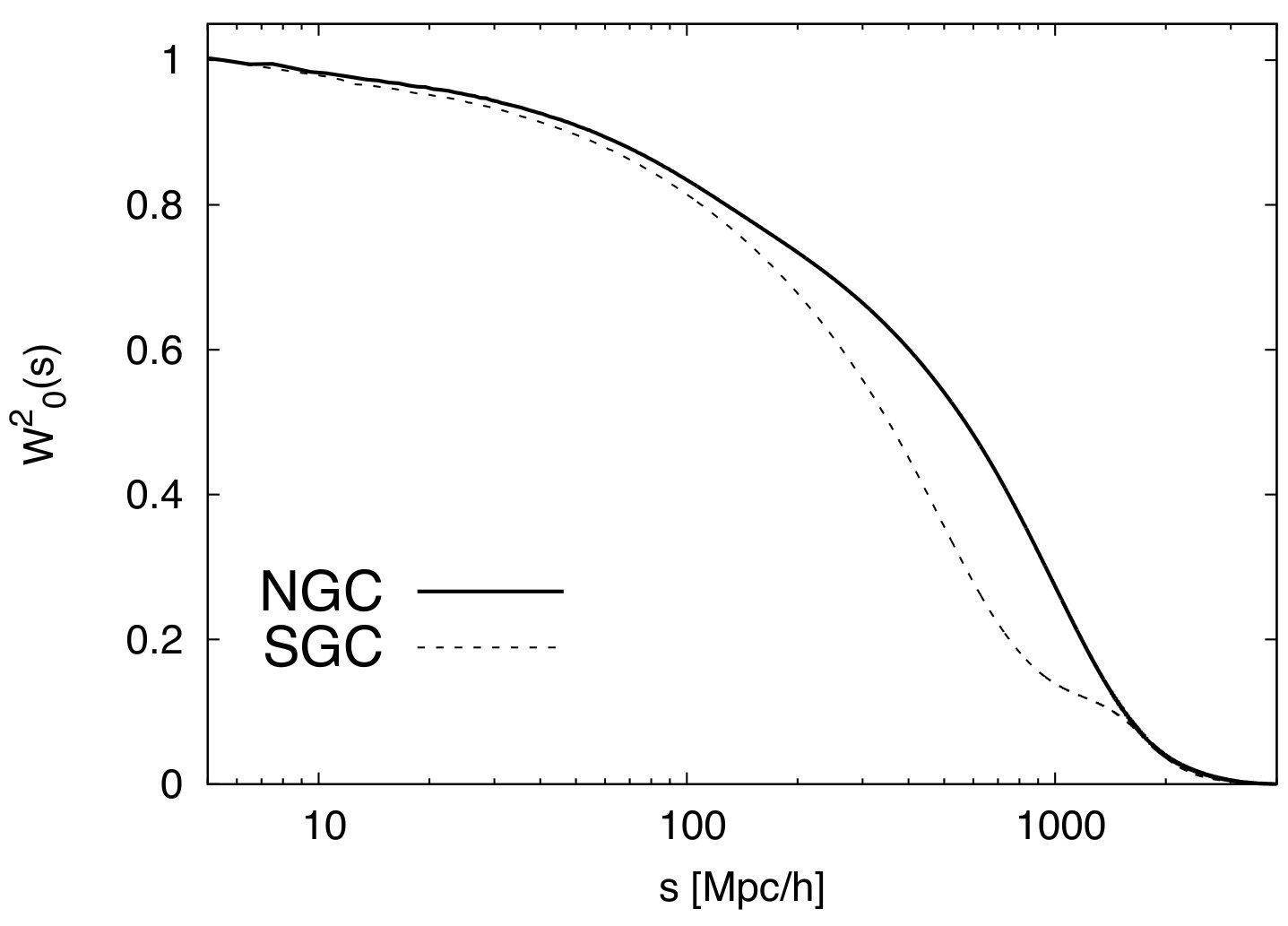 Figure 18
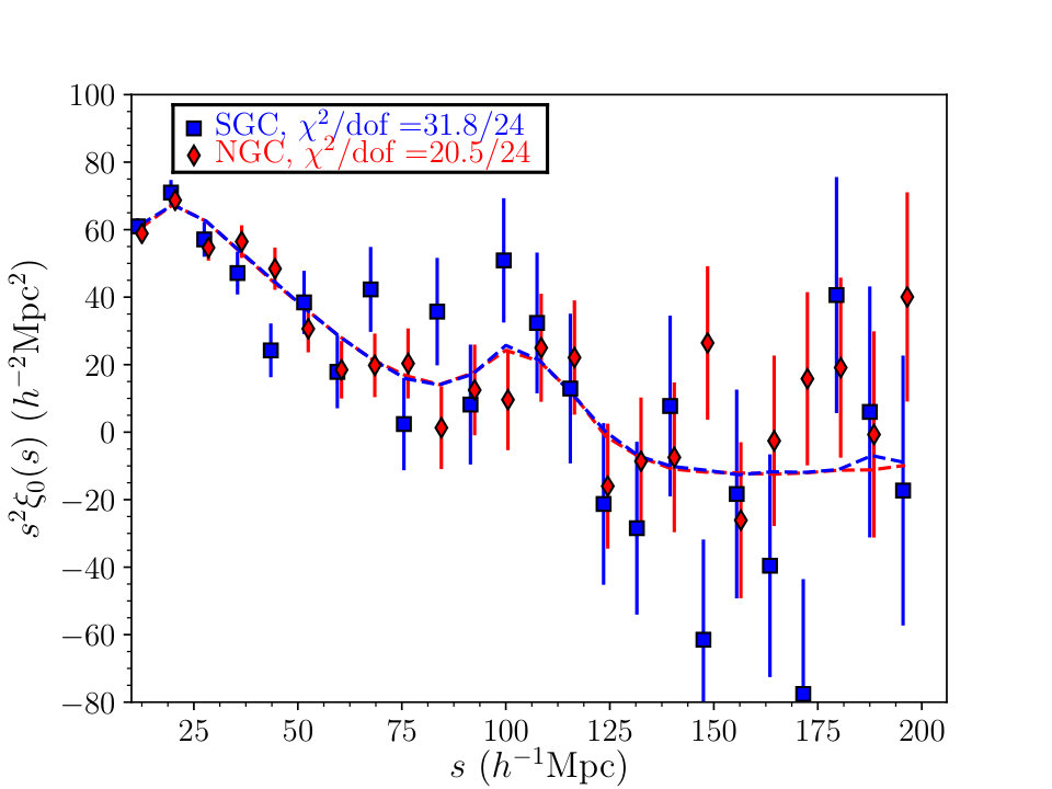 Figure 19
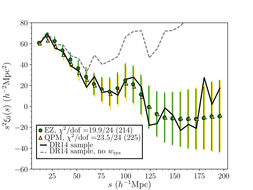 Figure 20
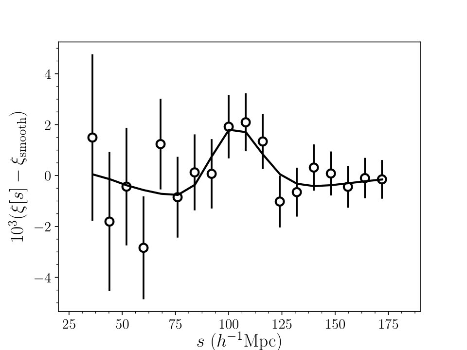 Figure 21
| NGC | SGC | Total | |
|---|---|---|---|
| 116866 | 77935 | 194801 | |
| 78425 | 58277 | 136702 | |
| 38441 | 19658 | 58099 | |
| 3598 | 2865 | 6463 | |
| 3126 | 2352 | 5478 | |
| 8908 | 5564 | 14472 | |
| 3782 | 4517 | 8299 | |
| 123903 | 82876 | 206779 | |
| Unweighted area (deg2) | 1356 | 1035 | 2391 |
| Weighted area (deg2) | 1288 | 995 | 2283 |
| Weighted area post-veto (deg2) | 1215 | 898 | 2113 |
| case | (Mpc) | |||||
|---|---|---|---|---|---|---|
| fiducial | 0.31 | 0.676 | 0.022 | 0.06 eV | - | 147.78 |
| QPM | 0.31 | 0.676 | 0.022 | 0 | 1.00108 | 147.62 |
| EZ | 0.307 | 0.678 | 0.02214 | 0 | 1.00101 | 147.66 |
| case | |
|---|---|
| EZ mocks: | |
| : | |
| fiducial | |
| 5Mpc | |
| : | |
| fiducial | |
| & | |
| log - binning | |
| log - binning & | |
| , terms | |
| QPM mocks: | |
| : | |
| fiducial | |
| 5Mpc | |
| QPM cov | |
| : | |
| fiducial | |
| QPM cov |
| case (+bin shift) | ||||
|---|---|---|---|---|
| EZ mocks: | ||||
| consensus | 1.003 | 0.050 | 0.050 | 944/1000 |
| : | ||||
| combined | 1.003 | 0.049 | 0.049 | 939/1000 |
| fiducial | 1.002 | 0.048 | 0.050 | 932/1000 |
| +2 | 1.002 | 0.049 | 0.050 | 928/1000 |
| +4 | 1.002 | 0.048 | 0.050 | 938/1000 |
| +6 | 1.003 | 0.048 | 0.051 | 929/1000 |
| 5Mpc | 1.003 | 0.049 | 0.050 | 937/1000 |
| : | ||||
| combined | 1.002 | 0.052 | 0.050 | 941/1000 |
| fiducial | 1.002 | 0.051 | 0.051 | 929/1000 |
| +1/4 | 1.001 | 0.052 | 0.050 | 931/1000 |
| +2/4 | 1.004 | 0.051 | 0.049 | 935/1000 |
| +3/4 | 1.001 | 0.052 | 0.050 | 937/1000 |
| log - binning | 1.002 | 0.051 | 0.050 | 927/1000 |
| 1.002 | 0.051 | 0.051 | 934/1000 | |
| QPM mocks: | ||||
| : | ||||
| fiducial | 1.001 | 0.051 | 0.052 | 361/400 |
| 5Mpc | 1.000 | 0.050 | 0.051 | 355/400 |
| QPM cov | 1.002 | 0.051 | 0.052 | 369/400 |
| : | ||||
| fiducial | 0.998 | 0.049 | 0.051 | 354/400 |
| QPM cov | 0.999 | 0.049 | 0.049 | 359/400 |
| case | /dof | |
| DR14 Measurement | – | |
| (combined) | 6.2/13 | |
| (combined) | 27.7/33 | |
| Robustness tests | ||
| : | ||
| fiducial | 0.9960.039 | 8.6/13 |
| +2 | 0.9960.041 | 6.4/13 |
| +4 | 0.9840.033 | 3.2/13 |
| +6 | 0.9930.035 | 6.0/13 |
| (combined) | 0.9790.039 | 11.7/13 |
| NGC | 0.9750.054 | 9.4/13 |
| SGC | 1.0140.057 | 18.9/13 |
| QPM cov | 0.9940.037 | 9.6/13 |
| Mpc | 0.9900.036 | 15.6/24 |
| no | 0.9990.041 | 7.4/13 |
| Mpc | 0.9970.042 | 7.9/8 |
| Mpc | 0.9900.036 | 8.7/13 |
| Mpc | 1.0040.045 | 9.6/13 |
| 1.0040.039 | 9.5/16 | |
| no prior | 0.9970.037 | 8.8/13 |
| : | ||
| (combined) | 28.2/33 | |
| fiducial | 30.1/33 | |
| 25.4/33 | ||
| 25.0/33 | ||
| 30.3/33 | ||
| NGC | 15.8/16 | |
| SGC | 13.8/16 | |
| QPM cov | 29.7/33 | |
| log - binning | 31.6/39 | |
| log - binning, | 37.0/45 | |
| no | 29.2/33 | |
| 53.3/47 | ||
| 29.6/33 | ||
| 30.2/33 | ||
| 29.9/32 | ||
| terms | 20.6/29 | |
| no-mask | 28.4/33 |
Peer Reviews
No public reviews on file for this paper yet. If you reviewed it on a platform where reviews are public (OpenReview, ICLR, NeurIPS, ICML), you can paste yours below so the community can read it here.
Videos
No videos yet. Explain this paper in a talk, walkthrough, or lecture? Add one.
The clustering of the SDSS-IV extended Baryon Oscillation Spectroscopic Survey DR14 quasar sample: First measurement of Baryon Acoustic Oscillations between redshift 0.8 and 2.2
Metin Ata1, Falk Baumgarten1,2, Julian Bautista3, Florian Beutler4, Dmitry Bizyaev5,6, Michael R. Blanton7, Jonathan A. Blazek8, Adam S. Bolton3,9, Jonathan Brinkmann5, Joel R. Brownstein3, Etienne Burtin10, Chia-Hsun Chuang1, Johan Comparat11, Kyle S. Dawson3, Axel de la Macorra12, Wei Du13, Hélion du Mas des Bourboux10, Daniel J. Eisenstein14, Héctor Gil-Marín15,16, Katie Grabowski5, Julien Guy17, Nick Hand18, Shirley Ho19,20,21, Timothy A. Hutchinson3, Mikhail M. Ivanov22,23, Francisco-Shu Kitaura24,25, Jean-Paul Kneib8,26, Pierre Laurent10, Jean-Marc Le Goff10, Joseph E. McEwen27, Eva-Maria Mueller4, Adam D. Myers3, Jeffrey A. Newman28, Nathalie Palanque-Delabrouille10, Kaike Pan5, Isabelle Pâris26, Marcos Pellejero-Ibanez24,25, Will J. Percival4, Patrick Petitjean29, Francisco Prada30,31,32, Abhishek Prakash28, Sergio A. Rodríguez-Torres30,31,33, Ashley J. Ross27,4, Graziano Rossi34, Rossana Ruggeri4, Ariel G. Sánchez11, Siddharth Satpathy20,35, David J. Schlegel19, Donald P. Schneider36,37, Hee-Jong Seo38, Anže Slosar39, Alina Streblyanska24,25, Jeremy L. Tinker7, Rita Tojeiro40, Mariana Vargas Magaña12, M. Vivek3, Yuting Wang13,4, Christophe Yèche10,19, Liang Yu41, Pauline Zarrouk10, Cheng Zhao41, Gong-Bo Zhao13,4, Fangzhou Zhu42
1 Leibniz-Institut für Astrophysik Potsdam (AIP), An der Sternwarte 16, D-14482 Potsdam, Germany
2 Humboldt-Universität zu Berlin, Institut für Physik, Newtonstrasse 15,D-12589, Berlin, Germany
3 Department Physics and Astronomy, University of Utah, 115 S 1400 E, Salt Lake City, UT 84112, USA
4 Institute of Cosmology & Gravitation, Dennis Sciama Building, University of Portsmouth, Portsmouth, PO1 3FX, UK
5 Apache Point Observatory and New Mexico State University, P.O. Box 59, Sunspot, NM 88349, USA
6 Sternberg Astronomical Institute, Moscow State University, Universitetski pr. 13, 119992 Moscow, Russia
7 Center for Cosmology and Particle Physics, Department of Physics, New York University, New York, NY 10003, USA
8 Institute of Physics, Laboratory of Astrophysics, École Polytechnique Fédérale de Lausanne (EPFL), Observatoire de Sauverny, 1290 Versoix, Switzerland
9 National Optical Astronomy Observatory, 950 N Cherry Ave, Tucson, AZ 85719, USA
10 IRFU,CEA, Université Paris-Saclay, F-91191 Gif-sur-Yvette, France
11 Max-Planck-Institut für Extraterrestrische Physik, Postfach 1312, Giessenbachstr., 85748 Garching bei München, Germany
12 Instituto de Física, Universidad Nacional Autónoma de México, Apdo. Postal 20-364, México
13 National Astronomy Observatories, Chinese Academy of Science, Beijing, 100012, P.R. China
14 Harvard-Smithsonian Center for Astrophysics, 60 Garden St., MS #20, Cambridge, MA 02138, USA
15 Sorbonne Universités, Institut Lagrange de Paris (ILP), 98 bis Boulevard Arago, 75014 Paris, France
16 Laboratoire de Physique Nucléaire et de Hautes Energies, Université Pierre et Marie Curie, 4 Place Jussieu, 75005 Paris, France
17 LPNHE, CNRS/IN2P3, Université Pierre et Marie Curie Paris 6, Université Denis Diderot Paris, 4 place Jussieu, 75252 Paris CEDEX, France
18 Department of Astronomy, University of California at Berkeley, Berkeley, CA 94720, USA
19 Lawrence Berkeley National Laboratory, 1 Cyclotron Road, Berkeley, CA 94720, USA
20 Department of Physics, Carnegie Mellon University, 5000 Forbes Avenue, Pittsburgh, PA 15213, USA
21 Berkeley Center for Cosmological Physics, LBL and Department of Physics, University of California, Berkeley, CA 94720, USA
22 Institute of Physics, LPPC, École Polytechnique Fédérale de Lausanne (EPFL), CH-1015, Lausanne, Switzerland
23 Institute for Nuclear Research of the Russian Academy of Sciences, 60th October Anniversary Prospect, 7a, 117312 Moscow, Russia
24 Instituto de Astrofísica de Canarias (IAC), C/Vía Láctea, s/n, E-38200, La Laguna, Tenerife, Spain
25 Dpto. Astrofísica, Universidad de La Laguna (ULL), E-38206 La Laguna, Tenerife, Spain
26 Aix-Marseille Université, CNRS, LAM (Laboratoire d’Astrophysique de Marseille), 38 rue F. Joliot-Curie 13388 Marseille Cedex 13, France
27 Center for Cosmology and Astro-Particle Physics, Ohio State University, Columbus, Ohio, USA
28 Department of Physics and Astronomy and the Pittsburgh Particle Physics, Astrophysics and Cosmology Center (PITT PACC), University of Pittsburgh, 3941 O’Hara Street, Pittsburgh, PA 15260, USA
29 Institut d’Astrophysique de Paris, Université Paris 6 et CNRS, 98bis Boulevard Arago, 75014 Paris, France
30 Instituto de Física Teórica (UAM/CSIC), Universidad Autónoma de Madrid, Cantoblanco, E-28049 Madrid, Spain
31 Campus of International Excellence UAM+CSIC, Cantoblanco, E-28049 Madrid, Spain
32 Instituto de Astrofísica de Andalucía (CSIC), E-18080 Granada, Spain
33 Departamento de Física Teórica M8, Universidad Autónoma de Madrid, E-28049 Cantoblanco, Madrid, Spain
34 Department of Physics and Astronomy, Sejong University, Seoul 143-747, Korea
35 The McWilliams Center for Cosmology, Carnegie Mellon University, 5000 Forbes Ave., Pittsburgh, PA 15213, USA
36 Department of Astronomy and Astrophysics, The Pennsylvania State University, University Park, PA 16802, USA
37 Institute for Gravitation and the Cosmos, The Pennsylvania State University, University Park, PA 16802, USA
38 Department of Physics and Astronomy, Ohio University, 251B Clippinger Labs, Athens, OH 45701, USA
39 Brookhaven National Laboratory, Bldg 510, Upton, New York 11973, USA
40 School of Physics and Astronomy, University of St Andrews, St Andrews, KY16 9SS, UK
41 Tsinghua Center for Astrophysics and Department of Physics, Tsinghua University, Beijing 100084, China
42 Department of Physics, Yale University, 260 Whitney Ave, New Haven, CT 06520, USA Email: [email protected]: [email protected]: [email protected]
Abstract
We present measurements of the Baryon Acoustic Oscillation (BAO) scale in redshift-space using the clustering of quasars. We consider a sample of 147,000 quasars from the extended Baryon Oscillation Spectroscopic Survey (eBOSS) distributed over 2044 square degrees with redshifts and measure their spherically-averaged clustering in both configuration and Fourier space. Our observational dataset and the 1400 simulated realizations of the dataset allow us to detect a preference for BAO that is greater than 2.8. We determine the spherically averaged BAO distance to to 3.8 per cent precision: D_{V}(z=1.52)=3843\pm 147\left(r_{\rm d}/r_{\rm d,fid}\right)\Mpc. This is the first time the location of the BAO feature has been measured between redshifts 1 and 2. Our result is fully consistent with the prediction obtained by extrapolating the Planck flat CDM best-fit cosmology. All of our results are consistent with basic large-scale structure (LSS) theory, confirming quasars to be a reliable tracer of LSS, and provide a starting point for numerous cosmological tests to be performed with eBOSS quasar samples. We combine our result with previous, independent, BAO distance measurements to construct an updated BAO distance-ladder. Using these BAO data alone and marginalizing over the length of the standard ruler, we find at 6.6 significance when testing a CDM model with free curvature.
keywords:
cosmology: observations - (cosmology:) large-scale structure of Universe - (cosmology:) distance scale - (cosmology:) dark energy
††pagerange: The clustering of the SDSS-IV extended Baryon Oscillation Spectroscopic Survey DR14 quasar sample: First measurement of Baryon Acoustic Oscillations between redshift 0.8 and 2.2–References††pubyear: 2017
1 Introduction
Using Baryon Acoustic Oscillations (BAOs) to measure the expansion of the Universe is now a mature field, with the BAO signal having been detected and measured to ever greater precision using data from a number of large galaxy surveys including: the Sloan Digital Sky Survey (SDSS) I and II (e.g., Eisenstein et al. 2005; Percival et al. 2010; Ross et al. 2015), the 2-degree Field Galaxy Redshift Survey (2dFGRS) (Percival et al., 2001; Cole et al., 2005), WiggleZ (Blake et al., 2011), and the 6-degree Field Galaxy Survey (6dFGS) (Beutler et al., 2011). The Baryon Oscillation Spectroscopic Survey (BOSS) (Dawson et al., 2013), part of SDSS III (Eisenstein et al., 2011), built on this legacy to obtain the first percent level BAO measurements (Anderson et al., 2014). Results from the completed, Data Release (DR) 12, sample of BOSS galaxies were presented in Alam et al. (2016).
As well as using galaxies as direct tracers of the BAO, analyses of the Lyman- Forest in quasar spectra with BOSS have provided cosmological measurements at (e.g. Delubac et al. 2015; Bautista et al. 2017). However, between the current direct-tracer and Lyman- measurements there is a lack of BAO measurements. Using quasars111In this work ‘quasar’ is used as a synonym for quasi-stellar object (QSO) rather than quasi-stellar radio source; more specifically, we mean a high-redshift point source whose luminosity is presumably powered by a super-massive black hole at the centre of an unobserved galaxy. as direct tracers of the density field offers the possibility of observations, with the main hindrance being their low space density and the difficulty of performing an efficient selection. The extended-Baryon Oscillation Spectroscopic Survey (eBOSS; Dawson et al. 2016), part of SDSS-IV (Blanton et al., 2017), has been designed to target and measure redshifts for quasars at (including spectroscopically-confirmed quasars already observed in SDSS-I/II). Although the space density will still be relatively low (compared with the densities of galaxies in BOSS, for example), eBOSS will offset this drawback by covering a significant fraction of the enormous volume of the Universe between redshifts 1 and 2.
Quasars were selected in eBOSS using two techniques. A “CORE” sample used a likelihood-based routine called XDQSOz to select from optical imaging, combined with a mid-IR-optical colour-cut. An additional selection was made based on variability in multi-epoch imaging from the Palomar Transient Factory (Rau et al., 2009). These selections are presented in Myers et al. (2015), alongside the characterisation of the final sample, as determined by the early data. The early data were observed as part of SEQUELS (The Sloan Extended QUasar, ELG and LRG Survey, undertaken as part of SDSS-III and SDSS-IV; described in the appendix of Alam et al. 2015), which acted as a pilot survey for eBOSS. SEQUELS used a broader quasar selection algorithm than that adopted for eBOSS, and a subsampled version of SEQUELS forms part of the eBOSS sample.
In this paper we present BAO measurements obtained from eBOSS, using quasars from the DR14 dataset to measure the BAO distance to redshift 1.5. These measurements represent the first instance of using the auto-correlation of quasars to measure BAO and the first BAO distance measurements between . The low space density of quasars means that reconstruction techniques (Eisenstein et al., 2007) are not expected to be efficient, but we are still able to obtain a 4.4 per cent BAO distance measurement at greater than 2.5 significance. The results are an initial exploration of the power of the eBOSS quasar data set. We expect many forthcoming studies to further optimize these BAO measurements, measure structure growth, and probe the primordial conditions of the Universe.
This paper is structured as follows. In Section 2 we describe how eBOSS quasar candidates were ‘targeted’ for follow-up spectroscopy, observed, and how redshifts were measured. In Section 3, we describe how these data are used to create catalogs suitable for clustering measurements. Section 4, presents our analysis techniques, including explanations of our fiducial cosmology, how we measure clustering statistics, how we model BAO in these clustering statistics, and how we assign likelihoods to parameters that we measure. In Section 5, we describe the two techniques used to produce a total of 1400 simulated realizations of the DR14 quasar sample, i.e., ‘mocks’. Section 6 reviews tests of our methodology using mocks; these tests allow us to define our methodological choices for combining measurements from different estimators. Section 7 presents the clustering of the DR14 quasar sample and the BAO measurements, including numerous robustness tests on these measurements. We then present an updated BAO distance ladder and place our measurement in the larger cosmological context in Section 8. We conclude with a preview of forthcoming cosmological tests expected to be performed using eBOSS quasar data and additional tracers in Section 9.
2 Data
In this section, we review the imaging data that was used to define a sample of quasar candindate ‘targets’ intended for spectroscopy. We then describe how we obtain spectroscopy for each target and then identify quasars and measure redshifts from this output. The process of transforming these data into large-scale structure (LSS) catalogs is described in Section 3.
2.1 Imaging
All eBOSS quasar targets selected for LSS studies are selected on imaging from SDSS-I/II/III and the Wide Field Infrared Survey Explorer (WISE, Wright et al. 2010). We describe each dataset below.
SDSS-I/II (York et al., 2000) imaged approximately 7606 deg2 of the Northern galactic cap (NGC) and approximately 600 deg2 of the Southern galactic cap (SGC) in the photometric pass bands (Fukugita et al., 1996; Smith et al., 2002; Doi et al., 2010); these data were released as part of the SDSS Data Release 7 (DR7, Abazajian et al. 2009). SDSS-III (Eisenstein et al., 2011) obtained additional photometry in the SGC to increase the contiguous footprint to 3172 deg2 of imaging in the SGC, released as part of DR8 (Aihara et al., 2011), alongside a re-processing of all DR7 imaging. The astrometry of this data was subsequently improved in DR9 (Ahn et al., 2012). All photometry was obtained using a drift-scanning mosaic CCD camera (Gunn et al., 1998) on the 2.5-meter Sloan Telescope (Gunn et al., 2006) at the Apache Point Observatory in New Mexico, USA.
The eBOSS project does not add any imaging area to that released in DR8, but takes advantage of updated calibrations of that data. Schlafly et al. (2012) applied the “uber-calibration” technique presented in Padmanabhan et al. (2008) to Pan-STARRS imaging (Kaiser et al., 2010). This work resulted in an improved global photometric calibration with respect to SDSS DR8, which is internally applied to SDSS imaging. Residual systematic errors in calibration are reduced to sub per-cent level on all photometric bands (Finkbeiner et al., 2016), and poorly constrained zero-points are much improved. The photometry with updated calibrations was released with SDSS DR13 (Albareti et al., 2016).
The WISE satellite observed the entire sky using four infrared channels centred at 3.4 m (W1), 4.6 m (W2), 12 m (W3) and 22 m (W4). The eBOSS quasar sample uses the W1 and W2 bands for targeting; see Myers et al. (2015) for details. All targeting is based on the publicly available unWISE coadded photometry force matched to SDSS photometry presented in Lang (2014).
2.2 Spectroscopic Observations
Quasar target selection for eBOSS is described in Myers et al. (2015). Objects that satisfy the target selection and which do not have a previously known and secure redshift are flagged as and assigned optical fibers (via a process termed tiling - see Section 3.1), and selected for spectroscopic observation. Spectroscopy is collected using the BOSS double-armed spectrographs (Smee et al., 2013), covering the wavelength range 3600 to 10000 Å with R. In BOSS, the pipelines to process data from CCD-level to 1d spectrum level to redshift are described in Albareti et al. (2016) and Bolton et al. (2012).
We divide the sources of secure redshift measurement into three classes:
- •
Legacy: these are quasar redshifts obtained by SDSS I/II/III via non-eBOSS related progams;
- •
SEQUELS: these are quasar redshifts obtained from the Sloan Extended QUasar, ELG and LRG Survey (SEQUELS) (designed as pilot survey for eBOSS, again see Myers et al. 2015);
- •
eBOSS: these are previously unknown quasar redshifts obtained by the eBOSS project.
2.2.1 Legacy
The eBOSS program does not allocate fibers to targets previously observed that have a confident spectroscopic classification and a reliable redshift from previous SDSS observations. A target is considered to have a “confident” classification if neither nor are flagged in the bitmask. A target is considered to have a “good” redshift if it is not labeled or in the DR12 quasar catalog of Pâris et al. (2017a). These targets, collectively termed legacy, typically have good, visually inspected, redshifts collated from SDSS-I, II and III data. Redshifts acquired before BOSS are obtained from a combination of Schneider et al. (2010) and a catalogue of known stellar spectra from SDSS-I/II. Targets observed during BOSS that resulted in a confident spectral classification and redshift are documented in the DR12 quasar catalogue (DR12Q, Pâris et al. 2017a), and are not re-observed in eBOSS. These known objects are therefore flagged as either , or (see section 4.4 of Myers et al. 2015 for full details on how these flags are set). Targets that were previously observed in SDSS-I/II/III but failed to result in a confident classification (i.e., had at least one of or set) or a good redshift determination (i.e., were not labeled or in DR12Q) were targeted for re-observation by either SEQUELS or eBOSS.
2.2.2 SEQUELS
SEQUELS is a spectroscopic program started during SDSS-III that was designed as a pilot survey for eBOSS. The total program consists of 117 plates, 66 of which were observed during BOSS and are included in DR12 (Alam et al., 2015). The remaining 51 plates were observed during the 1st year of the eBOSS program and were released in DR13 (Albareti et al., 2016). The target selection for SEQUELS is by construction deeper and less constrained than the finalized eBOSS target selections, so only a (large) fraction of the SEQUELS targets satisfy the eBOSS final selection criteria.222See §5.1 of Myers et al. (2015) for full details of the minor selection differences between SEQUELS and the rest of eBOSS. The SEQUELS area is not re-observed in eBOSS and, for the purpose of these catalogues, we treat SEQUELS targets that pass the final eBOSS target selection in an identical manner to eBOSS targets in the eBOSS footprint.
EBOSS_TARGET0 holds the targeting flags for SEQUELS targets, whereas EBOSS_TARGET1 contains the targeting flags for eBOSS targets. In the target collate file and in the LSS catalogues, all targets that pass the eBOSS selection have the appropriate EBOSS_TARGET1 set, irrespective of whether they lie in the SEQUELS or eBOSS footprint. These flags match those that will exist in the publicly released catalogs.
2.2.3 eBOSS
The eBOSS project, naturally, represents the bulk of our observations — over 75 per-cent of new redshifts in the DR14 LSS catalogues were observed during the eBOSS program. The target selection algorithm for quasars includes both LSS and Lyman quasar targets. We use only the LSS quasars, which have the QSO_CORE bit set in the targeting flags. The DR14 sample includes two years of eBOSS observations.
2.3 Measuring Redshifts
Robust spectral classification and redshift estimation is a challenging problem for quasars. In particular, the number and complexity of physical processes that can affect the spectrum of a quasar make it difficult to precisely and accurately disentangle systemic redshift (i.e., as a meaningful indicator of distance) from measured redshift (e.g., Hewett & Wild 2010). SEQUELS observations taken during SDSS-III (representing around half of the SEQUELS program) were all visually inspected, and helped define our process for identifying quasar candidates. As detailed in Dawson et al. (2016), 91 per cent of quasar spectra targeted for clustering studies are securely classified with an automated pipeline (according to said pipeline) and less than 0.5 per cent of these classifications were found to be false when visually examined. The automated classification fails to report a secure classification in the remaining nine per cent of cases and these are visually inspected, which is able to identify approximately half of these as quasars.
Information on all eBOSS quasars is detailed in the DR14 quasar catalogue (DR14Q, Pâris et al. 2017b), the successor to DR12Q, with the important distinction that the vast majority of LSS quasars are not visually inspected. DR14Q combines the LSS pipeline and visual inspection results together and provides a variety of value-added information. In particular, it contains three automated estimates of redshift that we consider in our LSS catalogs:
- •
The SDSS quasar pipeline redshifts, denoted ‘ZPL’, and documented in Bolton et al. (2012). The pipeline uses a PCA decomposition of galaxy and quasar templates, alongside a library of stellar templates, to fit a linear combination of four eigenspectra to each observed spectrum.
- •
A redshift estimate based on the location of the maximum of the MgII emission line blend at Å , denoted ‘ZMgII’. The MgII broad emission line is less susceptible to systematic shifts due to astrophysical effects and, when a robust measurement of this emission line is present, it offers a minimally-biased estimate of a quasar’s systemic redshift (see e.g. Hewett & Wild 2010; Shen et al. 2016).
- •
A ‘ZPCA’ estimate, as documented in Pâris et al. (2017a). ‘ZPCA’ uses a PCA decomposition of a sample of quasars with redshifts measured at the location of the maximum of the MgII emission line, and fits a linear combination of four eigenvectors to each spectrum.
Whereas ZMgII offers the least biased estimate of the quasar’s systemic redshift, it is more susceptible to variations in S/N, and therefore ZPCA is able to obtain the accuracy of ZMgII with increased robustness provided by utilizing the information from the full spectrum (see Fig. 10 of Dawson et al. 2016).
DR14Q also contains a redshift, ‘Z’, which it considers to be the most robust of the available options, in that these redshifts are known to have the lowest rate of catastrophic failures (and can be any of the three options above, depending on the particular object). Further details will be available in Pâris et al. (2017b). We will test the robustness of our results to the redshift estimates by also testing BAO measurements where we use ZPCA as the redshift in all cases where it is available. Further tests, especially those focusing on the impact on redshift-space distortion (RSD) measurements, will be presented in Zarrouk et al. (in prep.).
The redshift distribution of the DR14 LSS quasar sample is displayed in Fig. 1. The curves show the result for the fiducial redshift sample. Our study uses the data with . The target sample selection was optimized to yield quasars with (Myers et al., 2015). At lower redshifts, morphological cuts affect the sample selection; at higher redshift the redshift measurement is less secure. We can securely select quasars to , but given that BAO at lower redshifts is better sampled by galaxies, we impose the cut. Affecting our choice of a high-redshift cut is that quasars with are used for Ly- clustering measurements and we wish to cleanly separate the two volumes used for BAO measurements333We are likely to re-evaluate this choice in future studies.. The data in the NGC (red) has a slightly greater number density than that of the SGC (blue). The imaging properties in the two regions are somewhat different, and, as explained in Myers et al. (2015), we expect a more efficient target selection (and thus yield of successful quasar redshifts) in the NGC. We describe weights that are applied to correct for the variations in targeting efficiency in Section 3.4.
3 LSS Catalogs
In this section, we detail how the quasar target and redshift information is combined to create LSS catalogs suitable for large-scale clustering measurements.444The catalogues will be available at this website https://data.sdss.org/sas/dr14/eboss/lss/, after eBOSS DR14 studies are complete. The clustering of the eBOSS quasar sample has already been studied by Rodríguez-Torres et al. (2016) and Laurent et al. (2017). LSS catalogs were generated for these studies in similar fashion to the methods we outline below, which are closely matched to the methods described in Reid et al. (2016). In particular, Rodríguez-Torres et al. (2016); Laurent et al. (2017) found that the clustering amplitude of the sample, and its redshift evolution, is consistent with the assumptions used in Zhao et al. (2016) and that the clustering can be modeled with the type of simulation techniques that have been successfully applied to galaxy samples.
3.1 Footprint
Targets that pass the target selection algorithm, and for which there are no known good redshifts, are fed into a tiling algorithm (Blanton et al., 2003), that allocates spectroscopic fibers to targets within a tile. Allocation is done in a way that maximises the number of fibers placed on targets, considering the constraints imposed by a pre-set target priority list and the exclusion radius around each fiber (Dawson et al., 2016). The algorithm is sensitive to the target density on the sky, so overdense regions tend to be covered by more than one tile. This overlap of tiles locally resolves some collision conflicts, but all others are dealt with separately. For eBOSS and SEQUELS, quasars can have collisions with fellow quasars or higher priority target classes. Collisions with other target classes (including Lyman) are simply deemed ‘missed’ observations and will be treated as random. Collisions with fellow quasars are termed fiber collisions or close pair collisions; see Section 3.3. Approximately 40% of the eBOSS area is covered by more than one tile.
We use the MANGLE software package (Swanson et al., 2008) to decompose the sky into a unique set of sectors, within each we compute a survey completeness. Within each sector we define the following:
- •
Nlegacy: the number targets with previously known redshifts (excluded from tiling);
- •
Ngood: the number of fibers that yield good quasar redshifts;
- •
Nzfail: the number of fibers from which a redshift could not be measured;
- •
Nbadclass: the number of targets with spectroscopic classification that does not match its target class, for our quasar sample, these are exclusively galaxies555While we exclude them from our analysis, these are likely an interesting sample of object.;
- •
Ncp: the number of targets which did not receive a fiber due to being in a collision group (or “close-pair”);
- •
Nstar: the number of spectroscopically confirmed stars;
- •
Nmissed: the number of quasar targets to be observed in the future or not observed because of a collision with a different eBOSS target class.
A summary of the above numbers in each of our target samples, summed over all sectors, is given in Table LABEL:tab:catalogues. We define a targeting completeness per sector and per target class as
[TABLE]
Thus, tracks the fiber-allocation completeness of the eBOSS spectroscopic observations. This is the completeness that defines the eBOSS mask and which will be later used to construct random catalogues with a matched on-sky completeness (see Section 3.5). Inspection of Eq. 1 reveals that is impacted only by ; objects that were not assigned a fiber due to a fiber collision are treated separately (see Section 3.3).
Legacy targets are 100% complete, since they have already been observed. In order to account for this, we follow the same procedure as in BOSS (Reid et al., 2016) and sub-sample legacy targets to match the value of CeBOSS in each sector. SEQUELS and eBOSS observations are very similar and thus we treat them the same way, without distinction in the LSS catalogues. We keep all sectors with C in the LSS catalogues; the average completeness of the remaining sectors is high, averaging 95 and 96 per-cent in the North and South Galactic caps, respectively. The footprint of the DR14 LSS catalogues, coloured by the value of in each sector, is shown in Fig. 2. The completeness is generally quite high, except around the edges of the footprint where future observations will overlap with the DR14 data. Veto masks have also been applied and are detailed in the following subsection.
Additionally, we define a redshift completeness per sector as
[TABLE]
which tracks the quasar redshift efficiency averaged over each sector. We use this completeness value only to remove sectors with C. Redshift failures themselves are corrected for separately (see Section 3.3).
3.2 Veto Masks
A number of veto masks are used to exclude sectors in problematic areas. For the DR14 quasar sample, we apply the same veto masks as in BOSS DR12 (Reid et al., 2016), removing regions due to:
- •
Bad photometric fields, including cuts on seeing and Galactic extinction. In total, this mask excludes approximately 5 per-cent of the area. Cuts on extinction and seeing are only significant in the SGC (3.2 per-cent of the SGC area is excluded by the seeing cut and 2.6 per-cent by the extinction cut).
- •
Bright stars, based on the Tycho catalog (Høg et al. 2000; excluding 1.8 per cent of the area);
- •
Bright objects, including, e.g., stars not in the Tycho catalog and bright galaxies (Rykoff et al. 2014; excluding 0.05 per cent of the area);
- •
Centerposts, which anchor the spectrographic plates and prevent any fibers from being placed there (excluding per cent of the area);
We use the Schlegel, Finkbeiner & Davis (1998) map to determine extinction values and we remove areas with . For seeing, we use the value labeled ‘PSF_FHWM’ in the catalogues and remove areas where is greater than 2.3, 2.1, 2.0 in the g, r, and i band, respectively. Further details on these masks and their motivation can be found in section 5.1.1 of Reid et al. (2016). The veto masks have been applied to Fig. 2. The large gap in coverage in the SGC at RA, Dec is due to the extinction mask. The horizontal striped patterns are due to the photometric bad fields or poor seeing in the SDSS imaging. The other veto masks are generally too small to be distinguishable.
3.3 Spectroscopic Completion Weights
The spectroscopic completeness of the sample is affected by multiple factors. Again, our process for accounting for this incompleteness matches that described in Reid et al. (2016). The simplest is that not all targets in a given sector have been observed. We account for this effect by down-sampling the random catalogs by the completeness fraction. Targets also lack redshifts due to fiber collisions and redshift failures, and we describe how these are treated below.
Not all observations yield a valid redshift. Redshift failures do not happen randomly on a tile (see e.g. Laurent et al. 2017), meaning they cannot be accounted for uniformly within a sector. Instead, as in previous BOSS analyses (e.g. Reid et al. 2016), we choose to transfer the weight of the lost target to the nearest neighbour with a good redshift and spectroscopic classification in its target class, within a sector (this can be a quasar, a star or a galaxy, provided it is targeted as a quasar). This weight is tracked by WEIGHT_NOZ () in the LSS catalogues. WEIGHT_NOZ is set to 1 by default for all objects, and incremented by for objects with a neighbouring redshift failure. The median separation between a redshift failure and its up-weighted neighbour is 0.06o. This corrective scheme assumes that the redshift distribution of the redshift failures is the same as that of the good redshifts. This is not expected to be strictly true, but assumed for simplicity, given the small number of targets that are corrected as redshift failures (approximately 3.4 per-cent in the NGC and 3.6 per-cent in the SGC). This concern does not affect out BAO analysis, but its impact on RSD analysis is currently being studied.
Targets missed due to fiber collisions do not happen randomly on the sky - they are more likely to occur in overdense regions. Targets lost to fiber collisions have therefore a higher bias than average, and we must apply a correction to account for this. We correct for these fiber collisions by transferring the weight of the lost target to the nearest neighbour of the same target class with a valid redshift and spectroscopic classification. This weight is tracked by WEIGHT_CP () in the LSS catalogues. Legacy targets are allowed to accrue close-pair correction weights, and legacy targets are downsampled such that the number of eBOSS-legacy close-pairs matches the number of close-pairs in eBOSS within each sector. Like WEIGHT_NOZ, it is set to 1 as default for all objects and incremented by for every neighbouring fiber collision. A total of 4.0 per cent of the eBOSS quasar targets are corrected as close-pairs in the NGC; this fraction is 3.0 per cent in the SGC.
Redshift failures are allowed to accrue weight from neighbouring close pairs, in which case the closest neighbour sees incremented by the total of redshift failure. For example, it is possible for a quasar target to be unobserved due to a collision with another quasar target. The observed quasar target is given , but we then fail to obtain a good redshift. The nearest neighbour to this observed quasar target is thus given .
Thus, each quasar is given a spectroscopic completeness weight, to be used for any counting statistics.
3.4 Systematic Weights for Dependencies on Imaging Properties
As described in Laurent et al. (2017), weights are required for the DR14 quasar sample in order to remove spurious dependency on the 5 limiting magnitude (‘depth’) and Galactic extinction. Quasars are more securely identified where the depth is best and Galactic extinction is the variable that we find most affects differences in depth between the SDSS imaging bands, as they were nearly simultaneously observed.
For the DR14 quasar sample, we define weights based on the depth in the -band, in magnitudes (including the effect of Galactic extinction on this depth), and the Galactic extinction in units , using the map determined by Schlegel, Finkbeiner & Davis (1998). These are the important observational systematics identified in Laurent et al. (2017). We define the weights based on the sample DR14 quasars with (already passed through the steps defined in the preceding section). Compared to Laurent et al. (2017), our results differ in that we use the full DR14 set (approximately doubling the sample size) to determine the weights and that we define the weights separately for the NGC and SGC. As in Ross et al. (2012, 2017) and Laurent et al. (2017), we define the weights based on fits to linear relationships. We first determine the dependency with depth and then with extinction, after applying the weights for depth. The total weight is the multiplication of the two weights. Thus
[TABLE]
where is the band depth (in magnitudes) and is the Galactic extinction (in ). The best-fit coefficients are for the NGC and for the SGC. The differences in the coefficients for the two regions make it clear it is necessary to separate them for analysis of the DR14 sample. Fig. 3 presents the relationship between the projected number density quasars and potential systematic quantities, combining the NGC and SGC. After weighting for depth and Galactic extinction (red squares) the systematic trends are removed.
Fig. 4 displays the relationship between quasar density and the depth when dividing the sample into four redshift bins. No systematic trends are apparent with redshift, suggesting that the systematic relationships do not need to be defined as a function of the colour/magnitude of the quasars. The for the null test for the quasars with is large — 25 for 10 degrees of freedom — but this result is dominated by a single 4 outlier at the worst depth. For the 9 bins at greater depth, the is 12. We will demonstrate that our results are robust to any fluctuations in density imparted by the depth fluctuations.
3.5 Random Catalogues
Random catalogues are constructed that match the angular and radial windows of the data, but with approximately 40 times the number density. Such catalogs are required for both correlation function and power spectrum estimates of the clustering of the DR14 quasar sample, as detailed in Section 4.
We begin by using the MANGLE software to generate a set of points randomly distributed in the eBOSS footprint, where the angular number density in each sector is subsampled to match the value of CeBOSS in that sector. We then run the random points through the same veto masks that are applied to the data (see Section 3.2). Finally, we assign each random point a redshift that is drawn from the distribution of data redshifts that clear the veto mask. The draws are weighted by the total quasar weight given by w, such that the weighted redshift distribution of data and randoms match.
4 Methodology
4.1 Fiducial Cosmology
We use a flat, CDM cosmology with , , \sum m_{\nu}=0.06\eV and , where the subscripts , and stand for matter, baryon and neutrino, respectively, and is the standard dimensionless Hubble parameter. These choices match the fiducial cosmology adopted for BOSS DR12 analyses (Alam et al., 2016). One set of mocks we use, the EZmocks (see Section 5.1), use the cosmology of MultiDark-PATCHY (Kitaura et al., 2014, 2016) used in previous BOSS analyses. The other set of mocks we use, QPM mocks (see Section 5.2), uses a geometry that matches our fiducial cosmology but with . The properties of the cosmologies we use are listed in Table LABEL:tab:cosmo. Following the values provided in Table LABEL:tab:cosmo, the BAO distance parameter at the effective redshift of the quasar sample, with (see Eq. 13 for definition), are for both the fiducial cosmology and for the QPM cosmology and for the EZ mocks cosmology. A separate factor entering our analysis is the value for the comoving sound horizon at the baryon drag epoch, ; this parameter sets the position of the BAO scale in our theoretical templates. The different cosmologies and lack of a neutrino mass in the mocks shift to be less than the fiducial by just over for each type of mock we use.
4.2 Clustering Estimators
We perform two complementary BAO analyses: i) in configuration space, where the observable is the angle (with respect to the line of sight) average (the monopole) of the correlation function; ii) in Fourier Space, where the observable is the monopole of the power spectrum. When the entire spectrum of frequencies and positions is considered, both correlation function and power spectrum contain identical information as one represents the Fourier transform of the other. However, since our spectral range is finite, the correlation function and power spectrum do not contain exactly the same information, although we expect a high correlation between results using either statistic. Long wavelengths are limited by the size of the survey and small wave-lengths are limited by the resolution of the analysis. Furthermore, we expect that any potential uncorrected observational or modelling systematics will affect the correlation function and power spectrum differently. Thus, by performing two complementary analyses and combining them we expect to produce a more robust final result.
For both analyses, we require the data catalogue, which contains the distribution of quasars (which can be an actual or synthetic distribution) and the random catalogue, which consists of a Poisson-sampled distribution with the same mask and selection function as the data catalogue with no other cosmological correlations. We count each data and random object as a product of weights. For the data catalogue, the total weight corrects for systematic dependencies in the imaging, and spectroscopic data, (see Section 3.4 and 3.3, respectively) multiplied by a weight, , that is meant to optimally ponderate the contribution of objects based on their number density at different redshifts. Conversely, for random catalogue, objects are weighted only by . The weight is based on Feldman et al. (1994) and defined as,
[TABLE]
where is the amplitude of the power spectrum at the scale at which the FKP-weights optimise the measurement. For the expected BAO signature in the DR14 quasar sample this is Mpc*-1* (Font-Ribera et al., 2014a), and therefore, we use . The FKP weights have only a small effect on our results, as the number density is both low and nearly constant, so the value of the weight varies by less than 10 per cent.
The total weight applied to each quasar is thus
[TABLE]
while for each random object, the weight is simply .
4.2.1 Configuration Space
For the configuration space analysis the procedure we follow is the same as in Anderson et al. (2014), except that our fiducial bin-size is 8 Mpc. We repeat some of the details here. We determine the multipoles of the correlation function, , by finding the redshift-space separation, , of pairs of quasars and randoms, in units Mpc assuming our fiducial cosmology, and cosine of the angle of the pair to the line-of-sight, , and employing the standard Landy & Szalay (1993) method
[TABLE]
where represents the quasar sample and represents the uniform random sample that simulates the selection function of the quasars. thus represent the number of pairs of quasars with separation and orientation . In order to minimize any noise coming from the finite size of the random catalog, the random catalogs are many times the size of the data catalogs and the resulting counts are normalized accordingly. For the DR14 data, we use a random sample that is 40 as large as the data, which we have found is sufficiently large for our results to have converged within their quoted precision. For the mocks, we use larger random samples, 100 for the EZmocks and 70 for the QPM mocks. This is due to the fact that we use a single random catalog for all mocks. This eliminates any noise in the covariance matrix we determine from the mocks due to the finite size of the random catalogs. However, in order to obtain results to the precision expected for the full ensemble of mocks (e.g., to test their mean results) we require a random sample many times larger than required for a single realization.
We calculate in evenly-spaced bins666The pair-counts are tabulated using a bin width of 1 Mpc and summed into x Mpc bins, allowing different choices for bin centres and widths. in , testing both 5 and 8 Mpc, and 0.01 in . We then determine even moments of the redshift-space correlation function via
[TABLE]
where and is a Legendre polynomial of order . In this work we only use the moment. By defining the monopole this way, we ensure an equal weighting as a function of and thus a truly spherically averaged quantity. This means any distance scale we measure based on the BAO position in matches our definition of (given in Eq. 13).
The resulting correlation function is displayed in Fig. 5, where it is also compared to the mean of the mock samples we use. We describe the measurements further in Section 7.1.
4.2.2 Fourier Space
In order to measure the power spectrum of the quasar sample we start by assigning the objects from the data and random catalogues to a regular Cartesian grid. This is the starting point for using Fourier Transform (FT) based algorithms. In order to avoid spurious grid effects we use a convenient interpolation scheme to smooth the configuration-space overdensity field.
We embed the entire survey volume into a cubic box with size , and subdivide it into cubic cells, whose resolution and Nyquist frequency are , and , respectively. To obtain the smoothed overdensity field, an interpolation scheme is needed for the particle-to-grid assignment. By choosing a suitable interpolation scheme we can largely reduce the aliasing effect to a negligible level for frequencies smaller than the Nyqvist frequencies, which in this case comprises the typical scales for the BAO analysis. Traditional interpolation schemes include the Nearest-Grid-Point (NGP), Cloud-in-Cell (CIC), Triangular-Shaped-Cloud (TSC) and Piecewise Cubic Spline (PCS). These options correspond to the zero-th, first, second and third order polynomial B-spline interpolations, respectively (see Chaniotis & Poulikakos 2004 for higher order interpolation schemes based on B-spline). Additionally, each of these interpolation schemes has an associated grid correction factor that has to be applied to the overdensity field in Fourier space (Jing, 2005). The higher the order of the B-spline polynomial used in the grid interpolation, the smaller the effect of the grid on the final measurement. Aliasing arises as an extra limitation which cannot be avoided by just increasing the order of the grid interpolation scheme. Since for cosmological perturbations the bandwidth is not limited above a certain maximum cutoff frequency, the unresolved small scale modes are spuriously identified as modes supported by the grid, resulting in a contamination of the power spectrum, typically at scales close to the Nyqvist frequency. Recently, Sefusatti et al. (2016) demonstrated that by displacing the position of the initial grid by fractions of the size of the grid cell the effect of the aliasing was greatly suppressed. This procedure is called interlacing and was originally presented in (Hockney & Eastwood, 1981). In particular, Sefusatti et al. (2016) found that when a 2-step interlacing was combined with a PCS interpolation, the effect of aliasing was reduced to a level below , even at the Nyquist scale.
In this work, we apply a -order B-spline interpolation to calculate the overdensity field on the grid. Additionally, we combine two cartesian grids, displaced by half of their grid size, to account for the aliasing effect. We have checked (by doubling the number of grid cells per side) that the effect of aliasing is totally negligible in the range .
After applying the grid interpolation, we obtain an overdensity field at each grid centre, (Feldman et al., 1994),
[TABLE]
The quantity is the total weight for the quasars at the grid location given by Eq (5), and are the number density at position of the quasars and random objects, respectively, is the ratio between the total weighted numbers of the quasars () and random () catalogues, i.e., . Same as for the calculation, we use a random sample with 40 the size of the DR14 data set, 100 the size of the mean EZmock, and 70 the size of the mean QPM mock. Therefore, e.g., for the data and for the EZmocks. The factor , normalizes the amplitude of the observed power in accordance with its definition in a quasar distribution with no survey selection,
[TABLE]
where, is the mean number density of quasars and the area of the survey in steradians. We perform this integration by sampling the mean number density of quasars in shells of and summing in the range .
In this work, we only present a measurement of the monopole (angle averaged with respect to the line of sight) of the power spectrum777Future eBOSS studies will use the anisotropic signal.. To measure the power spectrum monopole, we must perform the Fourier transformation of the overdensity field defined in Eq (8). Since we are interested in the monopole, the varying line-of-sight of the quasars has no effect on our calculation. Specifically, we need to calculate the following quantity,
[TABLE]
The power spectrum monopole is evaluated by a summation over -directions and in the defined -bin,
[TABLE]
where is the mean of all values summed in the above equation.
We perform the measurement of binning linearly in bins of between and the Nyqvist Frequency. Within this wide range, we limit the BAO analysis to the frequencies . Scales outside of this range contain negligible information on the BAO peak position. We have checked these statements by using the mock quasar catalogues. The resulting power spectrum contains 21 -bins and is displayed in Fig. 6, where it is also compared to the mean of the mock samples. We describe these results further in Section 7.1.
4.3 BAO Modeling
We use the same basic modeling template of the BAO signal for both configuration and Fourier space. The BAO model is determined in Fourier space and then either transformed to configuration space or passed through the window function in order to be compared to observations. For both approaches, we determine how different the BAO scale is in our clustering measurements compared to its location in a template constructed using our fiducial cosmology. There are two main effects with cosmological dependence888There is a third effect, which is a small shift in the BAO position due to non-linear evolution, described later in this section. It has minor dependence on cosmology and its total effect is negligible compared to the precision of our measurements, which we demonstrate in later sections. that determine the difference between the observed BAO position and that in the template. The first effect is the difference between the BAO position in the true intrinsic primordial power spectrum and that in the model, with the multiplicative shift depending on the ratio , where is the sound horizon at the drag epoch (and thus represents the expected location of the BAO feature in co-moving distance units, due to the physics of the early Universe). The second effect is the difference in projection. The data are measured using a fiducial distance-redshift relation, matching that of the template: if the actual cosmology is different than that assumed we expect a shift that depends on in the radial direction, and in the angular direction. For spherically averaged clustering measurements, we thus measure
[TABLE]
with
[TABLE]
Given sufficient signal-to-noise ratio, and can be measured separately by using the isotropic and anisotropic signal. In this paper we only focus on the isotropic signal due to limited signal-to-noise ratio, and hence, we constrain .
The methodology we adopted to measure is based on that used in Anderson et al. (2014) (and references therein). We generate a template BAO feature using the linear power spectrum, , obtained from Camb999camb.info (Lewis et al., 2000; Howlett et al., 2012) and a ‘no-wiggle’ obtained from the Eisenstein & Hu (1998) fitting formulae101010In order to best-match the broadband shape of the linear power spectrum, we use , to be compared to 0.97 when generating the full linear power spectrum from camb. for and following Kirkby et al. (2013) for , both using our fiducial cosmology (except where otherwise noted).
Again emulating Anderson et al. (2014) (and references therein), given and , the linear theory BAO signal is described by the oscillation pattern in the . We account for some non-linear evolution effects by ‘damping’ this BAO signal:
[TABLE]
This damping is treated slightly different in the and analyses, as we describe in Sections 4.3.1 and 4.3.2. In addition to damping the BAO oscillations, non-linear evolution effects are also expected to cause small shifts (of order 0.5 per cent) in the BAO position (Padmanabhan & White, 2009), which should have a small cosmological dependence (e.g., the size of the shift is likely dependent on ). We will show that our results are insensitive to such effects.
4.3.1 Correlation Function Modeling
For the correlation function, we simply use
[TABLE]
and its Fourier transform in order to obtain the configuration-space BAO template, . We fix Mpc in the analysis and show that the results are insensitive to this choice. This choice is based on basic extensions of linear theory and the fact that the quasar sample has non-negligible redshift uncertainty. Seo & Eisenstein (2007) provide predictions and . This decomposition accounts for redshift-space distortions; the real-space prediction is given by . The spherical average is . For our fiducial cosmology, Mpc and Mpc. We compare these predictions to those obtained from real-space non-linear power spectrum predictions using Blas et al. (2016)111111Blas et al. (2016) also includes the shift in the BAO peak, due to the non-linear growth of the matter power spectrum, which we evaluate in Section 6., evaluated at using FAST-PT (McEwen et al., 2016). A value of Mpc produces a BAO feature in our template defined by Eq. 14, matching the amplitude of the Blas et al. (2016) template, suggesting reasonable agreement with the more basic Seo & Eisenstein (2007) approach. Thus, we expect Mpc for redshift-space measurements; we increase this to Mpc in order to account for redshift uncertainties. We test and discuss this issue further in Section 6.
Given , we then fit to the data using the model
[TABLE]
Including the polynomial makes our results insensitive to shifts in the broad-band shape of the measured . As in previous analyses (e.g., Anderson et al. 2014), we apply a Gaussian prior of width 0.4 around the obtained when fitting to the data in the range Mpc (not including the polynomial terms). These scales are safely outside of the scales where the BAO feature is significant. Using this prior ensures that the BAO feature in the model is neither unphysically large or small.
For both mocks and for the data, we adopt the appropriately weighted average of the NGC and SGC in order to obtain our BAO measurements. The configuration-space analysis does not have the Fourier-space window function concerns discussed in the following section. Thus, each correlation function BAO fit has five free parameters.
4.3.2 Power Spectrum Modelling
In the power spectrum analysis, the position of the BAO peak is described by the oscillation pattern in . The position of the peak is identified by shifting the pattern through the parameter as . We use the same power spectrum template form used for previous BAO fits in the BOSS survey (Gil-Marín et al., 2015),
[TABLE]
where the accounts for all the non-linear and redshift space effects in the power spectrum monopole. It is possible to model with higher polynomial coefficients such as . Although these terms were used for modelling the broadband power spectrum shape of the LRG galaxies at lower redshifts in BOSS (Gil-Marín et al., 2015), we have determined that for the current precision and redshift ranges in this paper, adding these two extra terms does not affect the determination of significantly.
The last step we need to incorporate in the model of Eq. 17 is the effect of the window function caused by the non-uniform angular distribution of quasars (see Fig. 2), and the dependence of the mean density of quasars with the radial distance (see. Fig. 1). These two effects are accounted for by following the procedure described in Wilson et al. (2017). The masked power spectrum, is written as a Hankel Transform (HT) of the masked correlation function ,
[TABLE]
where is the spherical Bessel function, , and can be written in terms of the correlation function -multipoles, corresponding to the inverse HT of the un-masked power spectrum template model,
[TABLE]
We neglect any contribution of the power spectrum quadrupole into the monopole through the window function, and therefore we approximate, . contains all the information on the radial and angular selection functions, and can be modelled either analytically or through the pair-counts of the random catalogue. For simplicity we follow the later option and we write as,
[TABLE]
where is normalised to 1 in the limit. The term in the denominator accounts for the volume of the shell when the binning is linear in .
The top panel of Fig. 7 displays the performance of for the redshift range , for the NGC and SGC patches, in solid and dashed black lines, respectively. In the case of no survey selection effect (for instance a periodic boundary condition simulation), the function would approach , and the convolution between a theoretical power spectrum and the FT of (a Dirac delta in this case) would produce no difference between the theoretical and the observed power spectrum. The effect of a non-flat redshift distribution and a non-uniform sky geometry produces a window function with the shape observed in the top panel of Fig. 7. As expected, the departure from the ideal case is more prominent in the SGC than in the NGS, as the SGC footprint covers a smaller angular area. The effect of the window function is to produce an extra coupling term (in addition to the non-linear coupling) among the -modes of the power spectrum. As a consequence, the covariance term is increased among -modes and the amplitude of the observed power spectrum is reduced at large scales, as it is shown in the bottom panel of Fig. 7.
Since the shape of the window function is slightly different for the NGC and SGC regions, we choose to perform the power spectrum BAO fit separately, assuming no correlation among the two disconnected regions. Furthermore, we fit for different broadband parameters in the NGC and SGC, to account for different observational effects, such as photometric calibration, that can yield to a different effective biases for the two separate regions. Thus, we fit for , , and separately for NGC and SGC, and keep the same value for and . Thus, in total we fit for 10 free parameters (9 if is kept constant) using 42 -modes (21 for each patch) in the range . We have observed that by following such approach the constraints on (in both mocks and data) are improved (when compared to the case where the weighted average is used in the fit) and that the resulting likelihoods are closer to a Gaussian distribution.
4.4 Parameter Estimation
We assume the likelihood distribution, , of any parameter (or vector of parameters), , of interest is a multi-variate Gaussian:
[TABLE]
The is given by the standard definition
[TABLE]
where represents the covariance matrix of a data vector and is the difference between the data and model vectors, when model parameter is used. We assume flat priors on all model parameters, unless otherwise noted.
In order to estimate covariance matrices, we use a large number of mock quasar samples (see Section 5), unless otherwise noted. The noise from the finite number of mock realizations requires some corrections to the values, the width of the likelihood distribution, and the standard deviation of any parameter determined from the same set of mocks used to define the covariance matrix. These factors are defined in Hartlap et al. (2007); Dodelson & Schneider (2013) and Percival et al. (2014); we apply the factors in the same way as in, e.g., Anderson et al. (2014). For our fiducial results, we use 1000 mocks and 18 measurement bins (fitting to the weighted mean of the NGC and SGC results). For the analysis we fit NGC and SGC separately, which corresponds of using 1000 mocks and 21 measurement bins for each NGC and SGC regions. In both cases, the number of mock realisations is much larger than the number of measurement bins, implying the finite number of mocks has less than a 2 per cent effect on our uncertainty estimates. We observe that for both and analyses the corresponding covariance matrices are dominated by their diagonal elements.
The covariance matrix derived from the mocks is dominated by its shot noise component due to the low density of the quasars. On one hand, the EZ and QPM mocks have been produced to match the effective number of objects observed in the data sample ( in Table LABEL:tab:catalogues). On the other hand, the EZ and QPM mocks do not currently include the redshift failures and collision pair effects. Therefore, the actual number of quasars in the mocks matches the effective number of quasars on the data catalogue, which makes the total number of quasars in the mocks slightly higher than in the data. As a consequence, the diagonal and off-diagonal components of the covariance are underestimated approximately by the ratio between and in the range . In order to correct for this effect we re-scale the derived covariance elements by these factors when analyzing the DR14 data, which are 1.069 for the NGC and 1.073 for the SGC. Future eBOSS analyses will include these effects in the mocks (and therefore this correction will be unnecessary). Here, we use the simple scaling as it has only a 3 per cent effect on the recovered uncertainty.
5 Simulated Catalogs
We use two different methods to create a total of 1400 simulations of the DR14 quasar sample, which we refer to as ‘mocks’. In order to create this number of mocks, approximate methods are required. Our approach in this respect is similar to previous BOSS analyses (Manera et al., 2013; Anderson et al., 2014; Alam et al., 2016). The two methods used are ‘EZmock’ and ‘QPM’ and are described in the following sub-sections.
5.1 EZmocks
For this work, we construct 1000 light-cone mock catalogues covering the full survey area of DR14 (NGC+SGC) and reproducing the redshift evolution of the observed quasar clustering. These are created using the ‘EZmock’ (Effective Zel’dovich approximation mock catalogue, Chuang et al. 2015a) method. EZmocks are constructed using the Zel’dovich approximation of the density field. This approach accounts for non-linear effects and also halo bias (i.e. linear, nonlinear, deterministic, and stochastic bias) into an effective modeling with few parameters, which can be efficiently calibrated with observations or N-body simulations. Chuang et al. (2015b) demonstrates that the EZmock technique is able to precisely reproduce the clustering of a given sample (including 2- and 3-point statistics) with minimal computational resources, compared to other methods. We use an improved version of EZmock code with respect to the one described in Chuang et al. (2015a). In our work, we assign the positions of quasars to simulated dark matter particles instead of populating them following a cloud-in-cell distribution. With this change, we do not need to enhance the BAO signal in the initial conditions, as done in Chuang et al. (2015a).
For this study, we calibrate the bias parameters with the observed DR14 eBOSS quasar clustering directly. The NGC and SGC regions are created from separate simulations and are treated independently, with bias values fit to the measured clustering and the taken as in Fig. 1. Comparisons between the mean clustering in the EZmock samples and the measured eBOSS clustering can be found in Figs. 5 and 6, demonstrating that a good match has been produced. The EZmocks use the same initial power spectrum used by the mock catalogues of the final BOSS data release (DR12; Kitaura et al. 2016; Alam et al. 2016). The fiducial cosmology model is CDM with =0.307115, =0.6777, =0.8225, =0.048206, =0.9611 (see Kitaura et al. 2016 for details).
Each light-cone mock constructed for this work is composed of 7 redshift shells. The redshift shells for a given light-cone mock are computed using different EZmock parameters but they share the same initial Gaussian density field so that the background density field is continuous. Each redshift shell is taken from one corresponding EZmock periodic box with the size of (5Gpc)3. For this study, we generated 10007(shells)2(NGC+SGC)14,000 EZmock boxes in total. We use the code make_survey Carlson & White (2010); White et al. (2014) to construct each redshift shell from the corresponding box.
In order to determine the redshift evolution of each EZmock parameter, we need to measure/determine the parameters at different redshifts. However, the clustering measurements from the observation corresponding to each redshift shell are too noisy to be used to determine the EZmock parameter values. Therefore, we use samples from overlapping redshift bins to measure the EZmock parameters at different redshift and do a proper inter- or extra- polation to determine the parameters for all the 7 redshift shells. For each EZmock parameter , we assume that its functional dependency is well approximated by
[TABLE]
where
[TABLE]
of the number count within a given redshift bin (with bin size ).
For this work, we measured the EZmock parameters from observation in the following three redshift ranges: , , and , respectively. We determine the , , and by solving the following equations
[TABLE]
Having solved the system of Eqs. 25 for the coefficients , and , Eq. 23 is used to determine an EZmock parameter value for any given redshift shell.
Fig. 8 compares the linear bias measured from EZmocks used in this work with the other measurements (Croom et al., 2005; Laurent et al., 2017). For each redshift shell, the bias is measured from the 1000 EZmock boxes. The EZmock parameters have been calibrated using the observed data in three redshift bins as described above, so that EZmocks present a consistent linear bias evolution in comparison with other works. More details of the algorithm, clustering performance, and tests on bias evolution will be provided in Chuang et al. (in prep.).
5.2 QPM Mocks
Quick Particle Mesh (QPM) mocks follow the method of White et al. (2014). In brief, QPM uses a low-resolution particle mesh gravity solver to evolve a density field forward in time. This approach captures the non-linear evolution of the density field, but does not have sufficient spatial or mass resolution to form dark matter halos. Particles are sampled from the density field in a fashion to approximate the distribution of small-scale densities of halos. This process mimics both the one-point and two-point distributions of halos—their mass function and bias function. This approximate halo catalog can then be treated in the same manner as that from a high-resolution simulation and populated with galaxies according to a halo occupation distribution (HOD; c.f. Tinker et al. 2012). For the mocks used in this paper, we have adjusted the parameters of White et al. (2014) that map local density to halo mass to account for the change in redshift ( rather than in White et al. 2014), as well as extending this mapping to lower halo masses, as required by the halos occupied by quasars.
To parameterize the halo occupation of quasars, we use the five-parameter HOD presented in Tinker et al. (2012), which separates objects into central quasars and satellite quasars. To determine the HOD of the DR14 quasar sample, the peak of the curve is the number density that the HOD is required to match. This number, in addition to the quasar large-scale bias measurement of allows us to determine the duty cycle of quasars. In the HOD context, the duty cycle is the fraction of halos that have quasars at their centres. There is some extra freedom due to the fraction of quasars that are satellites in larger halos, but this population is a minority of quasars. The left-hand side of Fig. 9 shows the HOD that matches both the peak of and (Laurent et al., 2017) with a satellite fraction of 0.15. The right-hand side of Figure 9 compares the projected correlation function predicted by this HOD to measurements of quasar clustering from Kayo & Oguri (2012) and Ross et al. (2009). Although the quasar selection algorithms for these two papers are markedly different from eBOSS DR14, both yielding much smaller number densities than the DR14 sample, the measured clustering is remarkably similar to that predicted by the HOD model. The smaller number density in the Ross et al. (2009) and Kayo & Oguri (2012) samples would be reflected in a lower duty cycle, with limited impact on the amplitude and shape of clustering.
The implementation of the HOD used here assumes no correlation between the occupation of central and satellite quasars; i.e., the presence of a satellite quasar is not conditioned on the existence of a central quasar in a given halo. This assumption is also borne out by Fig. 9—if all satellites were required to exist in halos with a central quasar, the amplitude of at Mpc would be larger by a factor of 100 while the large-scale bias would be unchanged. Such a dramatic change in the shape of quasar clustering is clearly not allowed by the data.
We simulated 100 cubic boxes of size . The boxes are remapped to fit the volume of the full planned survey using the code make_survey Carlson & White (2010); White et al. (2014). The same 100 cubic boxes are used for the Northern and Southern Galactic caps. The analysis presented here is based on the first two years of eBOSS data and therefore on a smaller volume. This situation allows to use different parts of a single QPM box to produce different realizations. Changing the orientation of the original box, we identified four configurations with less than 1.5 per cent overlap. We used these configurations to produce 400 QPM mocks per Galactic cap. The overlap between SGC and NGC can be as high as 10 per cent, but we identified pairs of configurations where the overlap is kept below 2 per cent. In this way we are able to compare Fourier space and configuration space results for the whole survey on a mock-by-mock basis (see Section 6).
We transform the boxes to mock catalogs in the following manner. Cartesian comoving coordinates of the cubic boxes are transformed to angular coordinates and radial distances using a flat CDM cosmology defined in Table LABEL:tab:cosmo. Objects outside the angular mask are removed and veto masks accounting for bright stars, bright objects, plates centerposts and bad photometric fields are applied in the same manner as for the data (see Section 3.2). The number density of quasars is downsampled to fit the redshift distribution (see Fig. 1) and FKP weights are calculated using the same value of (see Eq. 4). Furthermore, redshifts are smeared according to a Gaussian distribution of width taken from the eBOSS early analysis Dawson et al. (2016), namely km s*-1* for and km s*-1* above.
6 Tests on Mocks
We test our methodological choices by analyzing our mock catalogs and the robustness of the results to these different choices. These tests inform our decisions about how to combine results from different clustering estimators. When quoting uncertainties, we use half the width of the region, matching the approach of Ross et al. (2015). This choice best extrapolates to the expectation for data with greater signal to noise (e.g., future data releases), as the likelihood for BAO measurements is generally wider than a Gaussian distribution121212This effect is negligible for high signal-to-noise ratio measurements, such as those in Alam et al. (2016)..
We first consider the results obtained from the mean of the mock samples, which are listed in Table LABEL:tab:baomockmean. For , we subtract the expected value of 1.0010 from the EZ mocks and and 1.0011 for the QPM mocks. All of the mean mock results are biased to be high, by between 0.001 and 0.004. The correlation function and power spectrum results show good agreement, with negligible differences in and its uncertainty for our fiducial cases.
Non-linear structure growth is expected to produce such slightly biased values, of expected fractional size (Padmanabhan & White, 2009), implying a shift of 0.13 per cent for the DR14 quasar sample. We test this assumption by using Blas et al. (2016) to produce a BAO template that incorporates the expected non-linear structure growth effects. We compare this result to our template given by Eq. 14 with Mpc, as such a value yields a BAO feature of matching size. We measure a shift between the two templates of 0.07 per cent, which represents the prediction for the shift in for the matter power spectrum. Padmanabhan & White (2009) demonstrate the expected shift is roughly proportional to the bias of the sample, as the shift can be explained by higher-order bias terms and these for dark matter halos are roughly proportional to the linear bias. Given that Laurent et al. (2017) obtains a bias of 2.45 for eBOSS quasars, we should expect roughly 0.2 per cent shifts in the recovered from our fiducial template (which includes no shifts due to non-linear structure growth). This prediction is generally consistent with our results when using the mean of the mocks. The differences in these tests, compared with the expected , are at most 2 in terms of the ensemble of mocks being tested and never more than 0.1 compared to the expected result for a single realization. We thus consider any potential bias due to non-linear structure growth to be negligible given the uncertainty obtained from the DR14 quasar sample.
In order to test the effect of redshift uncertainties, we have run the QPM mocks with a variety of assumptions on the redshift uncertainty; full details can be found in Zarrouk et al. (in prep.). We simply consider the fiducial case, with redshift uncertainty matching Fig. 11 of Dawson et al. (2016) and a case without any redshift uncertainty. Without any redshift uncertainty, the mean of the QPM mocks is best-fit by Mpc; with the redshift uncertainty, the best-fit is Mpc. These results suggest our choice to use Mpc is slightly conservative (greater leads to a greater uncertainty obtained from the likelihood).
Table LABEL:tab:baomock displays the results obtained when fitting each individual mock. Here, we only report statistics for mocks that have a on both sides of the minimum , within our prior range of . We designate each such mock result a ‘detection’. Over 90 per cent of the mock samples satisfy this condition. For this reason, the mean s are slightly less than that obtained for the mean of the mock realizations (multiplying the uncertainty in Table LABEL:tab:baomockmean by ). The standard deviation of these samples is close to the mean uncertainty, as would be expected for a Gaussian distribution.
For the correlation function, the mean values are similar to those obtained when testing the mean of the mocks, as expected. We test bin sizes of 5Mpc and 8Mpc; the results are extremely similar and we thus choose 8Mpc binning as it represents the smaller data vector. The QPM and EZ mocks produce consistent results, suggesting the separate methods agree on the expected BAO signal-to-noise ratio in our DR14 quasar sample. In particular, the results for the QPM mocks are insensitive to whether we use the QPM mocks or the EZ mocks to construct the covariance matrix used for the fits. This suggests our results are robust to uncertainties in how we construct the covariance matrix.
For 8Mpc correlation function binning, results using different bin centres are not perfectly correlated. Instead, the correlation factors, when shifting by each available 2Mpc shift, are close to 0.9 (the range is 0.88 to 0.92). Thus, slightly improved results are obtained when combining the results of these four bin centres; for Gaussian distributions, we would expect a 4 per cent improvement given four measurements with correlation 0.9. We combine the results by simply taking the mean of the four likelihoods, matching the approach of Ross et al. (2015). This combination increases the number of detections from 932 to 939 and reduces the standard deviation from 0.050 to 0.049. These results are labeled ‘combined’ in Table LABEL:tab:baomock and represent our optimized method for measuring the correlation function BAO scale.
We find broadly consistent results in Fourier space. The fiducial power spectrum case recovers essentially the same number of detections (929 compared to 932) and has a slightly larger mean uncertainty and standard deviation. We test four bin centres for , shifting the centre by factors of 0.025Mpc*-1*. These results are more correlated than the bin centre results, as they range 0.94 and 0.96. Combining across the bin centre results by taking the mean of the four likelihoods increases the number of detections to 941 while keeping the mean uncertainty and standard deviation unchanged. The power spectrum results are consistent whether the QPM or EZ mocks are being tested, whether a logarithmic or linear -space binning is used, and whether the maximum -vector for the analysis is set to or .
We compare the and results directly for the cases where we averaged across the bin centres for the EZmocks (denoted ‘combined’ in Table LABEL:tab:baomock). The recovered are plotted against each other in the top panel Fig. 10, using steelblue circles. The results are strongly correlated (the correlation factor is 0.97) and are unbiased relative to each other. The bottom panel in Fig. 10 displays the uncertainty of the combined and results. The uncertainties are not as correlated as the best-fit , as the uncertainties obtained from the likelihoods are more narrowly distributed than the counterparts.
Given that the combined and produce slightly different likelihoods, but with strong correlation in the maximum likelihood, we adopt the mean of the and results as a ‘consensus’ measurement. Doing so, we obtain a slight increase in the number of detections (up to 944) and the standard deviation in the maximum likelihood value of matches the mean uncertainty obtained from the likelihood. Further, is distributed similarly to a unit Gaussian distribution, as shown in Fig. 11. These results suggest that the uncertainty we obtain by combining the and likelihoods are indeed good estimates of the uncertainty on for each mock realization. We copy this approach when obtaining our consensus results using the DR14 quasar data.
The tests presented in this Section define our procedure for obtaining BAO measurements from the data. The results suggest that there are no reasonable methodological choices that will affect our estimate of the uncertainty on our measurements by more than 10 per cent or bias our results by more than 0.1.
7 Results
7.1 Clustering Measurements
We measure the clustering of the DR14 quasar sample in the respective SGC and NGC regions, i.e., the window function is normalized in each respective region, and then the results are combined. In this section, we present the clustering measurements, in both configuration and Fourier space, comparing the results to each other and to the mock DR14 samples.
Fig. 5 displays the spherically averaged redshift-space correlation function of the DR14 quasar sample for the data in the SGC (blue squares) and NGC (red diamonds). The dashed curves display the mean of the 1000 EZmock samples. The data in each region is broadly consistent with the mean of the mocks and with each other. Each recovers a good when tested against the mean of the mocks, both when the NGC and SGC are combined and compared individually. We use the sum of the respective covariance matrices to test the consistency between the NGC and SGC, over the same range of scales. The is 30.0 for these 24 measurement bins, suggesting the clustering of the two regions is consistent.
The bottom panel of Fig. 5 displays the results combining NGC and SGC (now with a solid black curve for the data) and includes the mean of the QPM mocks for an additional comparison. The /dof, when comparing against both sets of mocks, is close to one and what appears to be the BAO feature can be seen at Mpc. In configuration space, the DR14 quasar clustering is consistent with the expected signal and noise. The grey dashed line in the figure displays the clustering of the DR14 quasar sample when the systematic weights (defined in Section 3.4) for depth and Galactic extinction are not used. The in comparison to the mocks is labeled in parentheses in the figure; it is worse by . This result is equivalent to having greater than a 13 effect, and can be compared to BOSS DR12, where the systematic weights had at most a 4 effect on the measured clustering (Ross et al., 2017).
Fig. 6 displays the same information as in Fig. 5, but in Fourier space. As expected, there is a similar consistency between the NGC and the SGC results, compared to each other and to the mean of the mock samples. For this comparison, we have added a constant value to the mock results; otherwise the agreement would not be so excellent. The mean of the mocks with no constant applied are shown by the dotted curves. We marginalize over a free constant term in the BAO analysis, and therefore believe this to be a fair comparison to evaluate the agreement, in terms of the signal relevant to the BAO measurement. Further, this difference in power clearly does not strongly affect the covariance matrix, as we obtained nearly identical results when fitting the QPM mocks when using either the QPM mocks or EZmocks to construct the covariance matrix. The effect of the systematic weights is negligible at scales Mpc*-1*; the result without applying the weights is barely distinguishable (it is plotted with a grey, dashed curve) and the comparison to the mean of the mock samples changes by at most 5.2 (when compared to the QPM mocks). These results imply that, while the effect of the systematic weights has great total significance, any effect on the measurement of the BAO scale is likely to be negligible.
7.2 BAO Measurements
Fig. 12 displays the measured BAO feature in the eBOSS DR14 quasar sample, using our fiducial analysis choices. The top panel shows the Fourier-space result and the bottom panel the result in configuration space. The BAO feature has been isolated in each case by subtracting the smooth component of the best-fit model; for , we also divide the results by the smooth component. A clear BAO feature is visible in both spaces.
The statistics for the BAO measurement can be found in top rows of Table LABEL:tab:baodata. These are the ‘combined’ results, where we have taken the mean likelihood across our four bin centres (as described in Section 6). For both and , the /dof is less than 1 and the precision is close to 4 per cent, with obtaining somewhat better precision (3.7 compared to 4.0 per cent). The two measurements differ by only 0.001 in . If anything, the agreement is surprisingly good. One can compare the orange star, representing our DR14 measurements, to the locus of mocks in the top panel of Fig. 10. The bottom panel of the same figure displays the comparison of the uncertainties we recover from each measurement. Our results are more precise than the average results but are clearly within the locus of points thus suggesting they are consistent with any expectations provided by our tests on mocks. We combine the two likelihoods and obtain a precision of 3.8 per cent. Translating this result to a distance measurement yields D_{V}(z=1.52)=3843\pm 147\left(r_{\rm d}/r_{\rm d,fid}\right)\Mpc.
Fig. 13 displays the likelihood and detection significance, in terms of , derived from the spherically-averaged correlation function (purple), power spectrum (burlywood), and their mean (black). The dashed curve represents the no BAO model; one can observe that the detection significance is greater than 2.8 for both and . All of the likelihoods are similarly skewed compared to a Gaussian, as large values of are not rejected to the same extent as low values. The black curve represents the eBOSS DR14 quasar BAO distance measurement. For any cosmological tests, we recommend directly using this likelihood, which is publicly available131313The BAO likelihood will be released publicly after the results are accepted by the journal for publication..
Robustness tests for our BAO measurements are shown in the bottom rows Table LABEL:tab:baodata. We find no particular causes for concern. Importantly, switching from our fiducial choice of redshift to shifts the recovered by only 0.012 (less than one third ) for both and and increases the mean of the and uncertainty from 0.038 to 0.040. These results have been combined across bin centres and can be compared directly to the DR14 results on the top lines of the table. The choice of redshift technique clearly does not have a strong impact on our results. Zarrouk et al. (in prep.) will examine this issue more closely in the context of RSD measurements, but we note that, e.g., we find no clear differences in the linear bias or excess large-scale clustering obtained using either redshift.
Additional robustness tests should be compared to the ‘fiducial’ results, which are the results for the fiducial choice of bin centre. The variations with bin centre for (labeled ) and (labeled ) are consistent with our findings testing our results with mocks; the mean of these four likelihoods is used as the DR14 measurement, labeled ‘combined’ in the top rows. Additional tests produce no changes that are greater than 0.2 for . For , the greatest change is only 0.3 when switching to logarithmic binning and increasing to 0.3Mpc*-1*. Finally, the results obtained from the independent NGC and SGC regions agree within 1, for both and
The systematic weights have negligible effects on our measurements, despite their enormous (13) effect on the large-scale correlation function of the DR14 quasar sample. We simply recover less than a 0.1 shift in and a 5 per cent increase in the uncertainty. The of the best-fit actually decreases (by 1), suggesting the effect of the depth and extinction systematics on our correlation function measurements are trivially accounted for with the polynomial terms in our BAO model.
For both and , there is a slight correlation between the assumed and the recovered that is less than 0.2 when testing in the range Mpc around our fiducial choice, with a similar impact on the size of the recovered uncertainty. For , we are able to marginalize over this parameter in the fit (using a Gaussian prior of Mpc) and we recover a result that matches the fiducial result with fixed at 6.0Mpc to better than 0.1. Thus, not only does the choice of have a minor effect on our analysis, our choice for its fiducial value is sufficiently close to the best-fit value as to not make a difference in our results.
Overall, the robustness tests suggest that our results are insensitive to arbitrary choices in the analysis or the way the catalog was constructed. This is consistent with Ross et al. (2017); Vargas-Magaña et al. (2016) who showed that systematic uncertainties are small compared to the BOSS DR12 statistical uncertainties. The BOSS DR12 precision is a factor of four better than our own, and thus makes these systematic uncertainties negligibly small for our analysis. A separate systematic uncertainty is the possible shift in the acoustic peak due to a coupling of the quasar density field to the small relative velocity between baryons and cold dark matter at high redshift (Tseliakhovich & Hirata, 2010; Dalal et al., 2010; Yoo et al., 2011; Slepian & Eisenstein, 2015; Blazek et al., 2016; Schmidt, 2016). This has been shown to be less than 0.5 per cent for low redshift galaxies (Yoo et al., 2013; Beutler et al., 2016; Slepian et al., 2016) and we expect it to be a minor effect for quasars with , compared to our statistical uncertainty. Further study is warranted, especially as the statistical uncertainty will be considerably improved with future datasets.
8 cosmological implications
In this section, we briefly discuss the cosmological implications of our DR14 quasar BAO measurement of D_{V}(z=1.52)=3843\pm 147\left(r_{\rm d}/r_{\rm d,fid}\right)\Mpc. We first present an updated BAO distance ladder and then demonstrate how this BAO distance ladder alone provides a powerful constraint on the geometry of the Universe.
Fig. 14 displays our spherically averaged BAO measurements overplotted with the CDM prediction from Planck (Planck Collaboration et al., 2015), compared to various similar measurements in the literature: the 6dFGS result from Beutler et al. (2011), the SDSS MGS result from Ross et al. (2015), the BOSS DR12 results from Alam et al. (2016), the WiggleZ results from Kazin et al. (2014), and the BOSS Ly from the combination of the Bautista et al. (2017) DR12 Ly auto-correlation and the Font-Ribera et al. (2014b) measurement using the cross-correlation of the Ly forest and quasars. Our measurement is in clear agreement with the expansion history predicted by Planck and other spherically averaged BAO distance measurements.
We have projected the combined Ly results onto a measurement, which brings them into agreement with the Planck prediction. These Ly measurements are in tension when considering their sensitivity to and separately. We do not attempt to perform this decomposition with the DR14 quasar sample, as its signal-to-noise ratio makes it difficult to perform this decomposition robustly with BAO-only measurements. This will be done with future eBOSS quasar studies incorporating the RSD signal or using larger data sets.
We use the BAO distance ladder to constrain the geometry of the Universe. To do so, we assume only that the BAO feature has a constant co-moving size; we assume no knowledge of the physics that produced the feature. We use an open CDM cosmology, which is parametrised using three parameters,
[TABLE]
where denotes the fractional energy budget contributed by dark energy, and the Hubble parameter. This approach matches that recently presented in Aubourg et al. (2015); Bautista et al. (2017). In this way, we are using only BAO measurements in order to test cosmology. We defer further study of the cosmological constraints afforded by our eBOSS DR14 quasar BAO measurement in combination with non-BAO data to future studies.
To obtain the constraint on and , which quantifies the cosmic geometry at the present epoch, we perform a Monte Carlo Markov Chain (MCMC) fitting using a modified version of CosmoMC (Lewis & Bridle, 2002), and marginalise over . The datasets we use are as follows,
- •
BOSS galaxies: The anisotropic BAO measurement from BOSS DR12 presented in Alam et al. (2016);
- •
BOSS galaxies+eBOSS: The isotropic BAO measurement D_{V}(z=1.52)=3843\pm 147\left(r_{\rm d}/r_{\rm d,fid}\right)\Mpc determined in this work combined with the BOSS DR12 BAO measurement;
- •
Full BAO: BOSS galaxies+eBOSS combined with the anisotropic BAO measurement from the DR11 Lyman- cross-correlation sample (Font-Ribera et al., 2014b) and the DR12 auto-correlation sample Bautista et al. (2017), and the isotropic BAO measurements using MGS (Ross et al., 2015) and 6dFGRS (Beutler et al., 2011) galaxy samples.
The 68 & 95% CL joint constraint on and , and the one-dimensional probability distribution of , are shown in Fig 15. The quasar BAO measurement in this work significantly improves the constraint, i.e.,
[TABLE]
where
[TABLE]
denotes the Figure of Merit (FoM) of the geometric constraint of the Universe. The significance of , in other words, the existence of dark energy, is raised from to CL when the eBOSS quasar BAO is added to BOSS galaxies. Despite its relative lack in precision, the eBOSS DR14 quasar BAO measurement is able to provide a significant improvement over the BOSS galaxy BAO measurements alone as it provides a high-redshift constraint. Importantly, using all BAO measurements to date (the Full BAO) sample, we reach a detection of dark energy using BAO alone; this considerable improvement is mainly provided by the higher redshift and more precise BOSS Ly measurements discussed earlier in this section141414The DR14 measurement does not provide a significant improvement over what is achieved without it but with Ly; c.f. Bautista et al. (2017).. Finally, all variations of the data set tested are in full agreement with a flat geometry.
BAO distance measurements continue to be in broad agreement with the flat CDM model and the best-fit parameters from the Planck mission (Planck Collaboration et al., 2015) assuming this model.
9 Conclusions
We have used a sample of 147,000 quasars distributed over more than 2000 deg2 in order to obtain the spherically-averaged BAO measurement D_{V}(z=1.52)=3843\pm 147\left(r_{\rm d}/r_{\rm d,fid}\right)\Mpc. We have demonstrated this measurement is robust against a variety of methodological and observational concerns and choices, once again demonstrating BAO distance measurements to be one of the most robust observational probes of dark energy (as shown/discussed previously in, e.g., Ross et al. 2012; Weinberg et al. 2013; Ross et al. 2017; Vargas-Magaña et al. 2016).
These results demonstrate that the BAO signal in the distribution of quasars is consistent with expectations of basic LSS predictions. The clustering we measure and its BAO signal are consistent with that in our mock realizations. While the formation and evolution of quasars remains an active research field, they are clearly not so exotic as to greatly disturb the BAO signal.
We combine our result with previous, independent, BAO distance measurements to construct an updated BAO distance-ladder. Using these BAO data alone, we tested a CDM model with free curvature, assuming only that the acoustic scale has a fixed comoving size. We found at 6.6 significance. Considering only BOSS galaxy and eBOSS quasar results, the significance remained greater than 3. All of our results are fully consistent with a flat geometry. BAO distance measurements, now across a broad range of redshifts, are in clear agreement with the flat CDM cosmological paradigm.
This work represents the first cosmological analysis to be done with eBOSS quasar data. We expect numerous studies to follow, both with this catalog and with future, larger data sets. In particular, given the wide redshift coverage of the eBOSS quasar sample, there is potentially ample tomographic information along the radial direction. This aspect is crucial to reconstruct the history of the cosmic expansion and structure growth, which is key for the probe of dynamical dark energy (Wang et al., 2016; Zhao et al., 2017a, b), modified gravity, and neutrino masses. We expect our DR14 results can be extended through the use of more optimal redshift-weighting methods for the BAO (e.g., Zhu et al. 2016; Wang et al. in prep.), redshift-space distortion (RSD) analyses, or their combination (Ruggeri et al., 2017). Additional BAO information can be extracted from higher-order statistics (Slepian et al., 2016). Further, we anticipate the enormous volume probed by the entire eBOSS quasar sample will afford a precise measurement the signature of primordial non-Gaussianity. The final eBOSS quasar sample is expected to have approximately three times the volume of the DR14 sample, and will thus provide exciting improvements in the statistical precision of our BAO measurement, even without the expected methodological improvements.
The direct use of quasars as a tracer represents only one facet of the eBOSS program. Separate analyses of the eBOSS luminous red galaxy (LRG) and emission line galaxy (ELG) samples will measure BAO and RSD signal at redshift 0.8, thereby filling the gap in redshift between BOSS galaxies and eBOSS quasars. Lyman forest studies using eBOSS observations of quasars at will improve BAO measurements at . Upcoming galaxy spectroscopic surveys will provide unprecedented precision; these include the Hobby-Eberly Telescope Dark Energy Experiment (HETDEX; Hill et al. 2008)151515http://hetdex.org/, Dark Energy Spectroscopic Instrument (DESI DESI Collaboration et al. 2016a, b)161616http://desi.lbl.gov/, Prime Focus Spectrograph (PFS; Tamura et al. 2016)171717http://pfs.ipmu.jp/ and the Euclid satellite mission (Amendola et al., 2013)181818https://www.cosmos.esa.int/web/euclid/. These surveys will probe the Universe using multiple tracers including quasars, ELGs and LRGs. The work we have presented, and eBOSS studies in general, represent an exciting first step in obtaining a densely sampled BAO distance ladder to .
acknowledgements
We thank the anonymous referee for comments that helped improve this paper.
AJR is grateful for support from the Ohio State University Center for Cosmology and ParticlePhysics.
HGM acknowledges support from the Labex ILP (reference ANR-10-LABX-63) part of the Idex SUPER, and received financial state aid managed by the Agence Nationale de la Recherche, as part of the programme Investissements d’avenir under the reference ANR-11-IDEX-0004-02.
GBZ is supported by NSFC Grant No. 11673025, and by a Royal Society Newton Advanced Fellowship.
RT acknowledges support from the Science and Technology Facilities Council via an Ernest Rutherford Fellowship (grant number ST/K004719/1)
CHC is grateful for support from Leibniz-Institut für Astrophysik Potsdam (AIP).
EB and PZ acknowledge support from the P2IO LabEx (ANR-10-LABX-0038).
JLT acknowledges support from National Science Foundation grant AST-1615997
YW is supported by the NSFC Grant No. 11403034
WJP acknowledges support from the UK Space Agency through grant ST/K00283X/1, and WJP acknowledges support from the European Research Council through grant Darksurvey, and the UK Science & Technology Facilities Council through the consolidated grant ST/K0090X/1.
ADM was partially supported by the NSF through grant numbers 1515404 and 1616168.
IP acknowledges the support of the OCEVU Labex (ANR-11-LABX-0060) and the A*MIDEX project (ANR-11-IDEX-0001-02) funded by the “Investissements d’Avenir” French government program managed by the AN
JPK acknowledges support from the ERC advanced grant LIDA.
GR acknowledges support from the National Research Foundation of Korea (NRF) through NRF-SGER 2014055950 funded by the Korean Ministry of Education, Science and Technology (MoEST), and from the faculty research fund of Sejong University in 2016.
Colours made possible by http://matplotlib.org/examples/color/named_colors.html; figures made colourblind-friendly (hopefully) by use of Color Oracle software.
Funding for SDSS-III and SDSS-IV has been provided by the Alfred P. Sloan Foundation and Participating Institutions. Additional funding for SDSS-III comes from the National Science Foundation and the U.S. Department of Energy Office of Science. Further information about both projects is available at www.sdss.org. SDSS is managed by the Astrophysical Research Consortium for the Participating Institutions in both collaborations. In SDSS-III these include the University of Arizona, the Brazilian Participation Group, Brookhaven National Laboratory, Carnegie Mellon University, University of Florida, the French Participation Group, the German Participation Group, Harvard University, the Instituto de Astrofisica de Canarias, the Michigan State / Notre Dame / JINA Participation Group, Johns Hopkins University, Lawrence Berkeley National Laboratory, Max Planck Institute for Astrophysics, Max Planck Institute for Extraterrestrial Physics, New Mexico State University, New York University, Ohio State University, Pennsylvania State University, University of Portsmouth, Princeton University, the Spanish Participation Group, University of Tokyo, University of Utah, Vanderbilt University, University of Virginia, University of Washington, and Yale University.
The Participating Institutions in SDSS-IV are Carnegie Mellon University, Colorado University, Boulder, Harvard-Smithsonian Center for Astrophysics Participation Group, Johns Hopkins University, Kavli Institute for the Physics and Mathematics of the Universe Max-Planck-Institut fuer Astrophysik (MPA Garching), Max-Planck-Institut fuer Extraterrestrische Physik (MPE), Max-Planck-Institut fuer Astronomie (MPIA Heidelberg), National Astronomical Observatories of China, New Mexico State University, New York University, The Ohio State University, Penn State University, Shanghai Astronomical Observatory, United Kingdom Participation Group, University of Portsmouth, University of Utah, University of Wisconsin, and Yale University.
This work made use of the facilities and staff of the UK Sciama High Performance Computing cluster supported by the ICG, SEPNet and the University of Portsmouth. This research used resources of the National Energy Research Scientific Computing Center, a DOE Office of Science User Facility supported by the Office of Science of the U.S. Department of Energy under Contract No. DE-AC02-05CH11231.
The reference list from the paper itself. Each links out to its DOI / PubMed record.
- 1Abazajian et al. (2004) Abazajian, K., Adelman-Mc Carthy, J. K., Agüeros, M. A., et al. 2004, AJ, 128, 502
- 2Abazajian et al. (2009) Abazajian, K., et al. 2009, Ap JS, 182, 543
- 3Ahn et al. (2012) Ahn, C. P., Alexandroff, R., Allende Prieto, C., et al. 2012, Ap JS, 203, 21
- 4Amendola et al. (2013) Amendola, L., Appleby, S., Bacon, D., et al. 2013, Living Reviews in Relativity, 16, 6
- 5DESI Collaboration et al. (2016 a) DESI Collaboration, Aghamousa, A., Aguilar, J., et al. 2016, ar Xiv:1611.00036
- 6DESI Collaboration et al. (2016 b) DESI Collaboration, Aghamousa, A., Aguilar, J., et al. 2016, ar Xiv:1611.00037
- 7Aihara et al. (2011) Aihara, H., Allende Prieto, C., An, D., et al. 2011, Ap JS, 193, 29
- 8Alam et al. (2015) Alam, S., Albareti, F. D., Allende Prieto, C., et al. 2015, Ap JS, 219, 12