
TL;DR
Matching logic is a versatile first-order logic variant that uses patterns for specifying and reasoning about structures, generalizing many logical frameworks and enabling effective program analysis.
Contribution
It introduces matching logic, a new logical framework that unifies various logics and simplifies reasoning about complex program structures through pattern matching.
Findings
Generalizes propositional logic, algebraic specification, and modal logic
Allows specification of separation requirements at any program level
Can be translated into predicate logic with equality for practical reasoning
Abstract
This paper presents matching logic, a first-order logic (FOL) variant for specifying and reasoning about structure by means of patterns and pattern matching. Its sentences, the patterns, are constructed using variables, symbols, connectives and quantifiers, but no difference is made between function and predicate symbols. In models, a pattern evaluates into a power-set domain (the set of values that match it), in contrast to FOL where functions and predicates map into a regular domain. Matching logic uniformly generalizes several logical frameworks important for program analysis, such as: propositional logic, algebraic specification, FOL with equality, modal logic, and separation logic. Patterns can specify separation requirements at any level in any program configuration, not only in the heaps or stores, without any special logical constructs for that: the very nature of pattern…
Click any figure to enlarge with its caption.
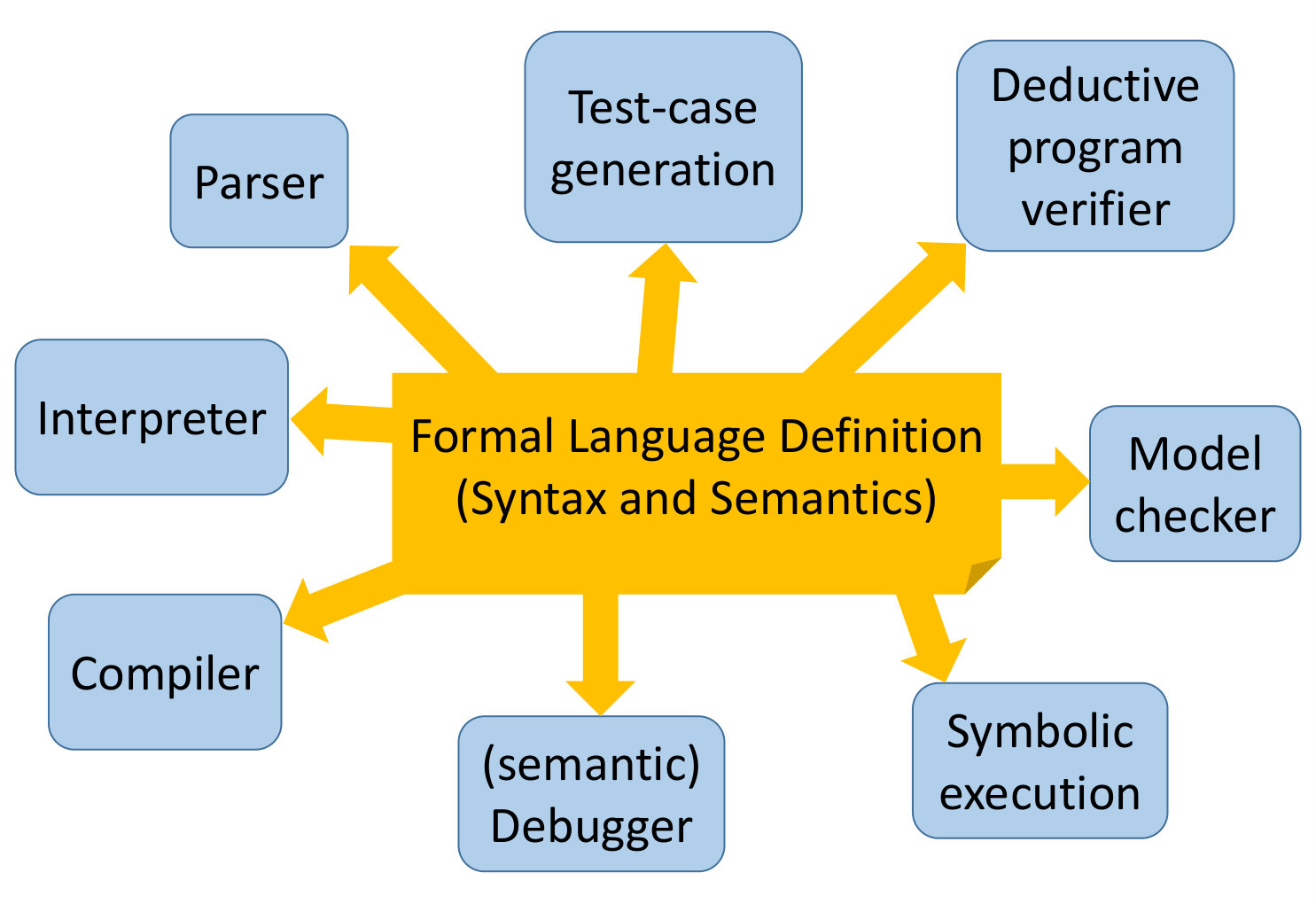 Figure 1
Peer Reviews
No public reviews on file for this paper yet. If you reviewed it on a platform where reviews are public (OpenReview, ICLR, NeurIPS, ICML), you can paste yours below so the community can read it here.
Videos
No videos yet. Explain this paper in a talk, walkthrough, or lecture? Add one.
Taxonomy
TopicsLogic, programming, and type systems · Formal Methods in Verification · Model-Driven Software Engineering Techniques
\lmcsheading
13(4:28)2017 1–LABEL:LastPage
Jan. 13, 2014 Dec. 20, 2017
\titlecomment\lsuper
*Extended version of an invited paper at the 26th International Conference on Rewriting Techniques and Applications (RTA’15), June 29 to July 1, 2015, Warsaw, Poland.
Matching Logic\rsuper*
Grigore Roşu
University of Illinois at Urbana-Champaign, USA
Abstract.
This paper presents matching logic, a first-order logic (FOL) variant for specifying and reasoning about structure by means of patterns and pattern matching. Its sentences, the patterns, are constructed using variables, symbols, connectives and quantifiers, but no difference is made between function and predicate symbols. In models, a pattern evaluates into a power-set domain (the set of values that match it), in contrast to FOL where functions and predicates map into a regular domain. Matching logic uniformly generalizes several logical frameworks important for program analysis, such as: propositional logic, algebraic specification, FOL with equality, modal logic, and separation logic. Patterns can specify separation requirements at any level in any program configuration, not only in the heaps or stores, without any special logical constructs for that: the very nature of pattern matching is that if two structures are matched as part of a pattern, then they can only be spatially separated. Like FOL, matching logic can also be translated into pure predicate logic with equality, at the same time admitting its own sound and complete proof system. A practical aspect of matching logic is that FOL reasoning with equality remains sound, so off-the-shelf provers and SMT solvers can be used for matching logic reasoning. Matching logic is particularly well-suited for reasoning about programs in programming languages that have an operational semantics, but it is not limited to this.
Key words and phrases:
Program logic; First-order logic; Rewriting; Verification
1991 Mathematics Subject Classification:
D.2.4 Software/Program Verification; D.3.1 Formal Definitions and Theory; F.3 LOGICS AND MEANINGS OF PROGRAMS; F.4 MATHEMATICAL LOGIC AND FORMAL LANGUAGES
The work presented in this paper was supported in part by the Boeing grant on "Formal Analysis Tools for Cyber Security" 2014-2017, the NSF grants CCF-1218605, CCF-1318191 and CCF-1421575, and the DARPA grant under agreement number FA8750-12-C-0284.
Contents
1. Introduction
In their simplest form, as term templates with variables, patterns abound in mathematics and computer science. They match a concrete, or ground, term if and only if there is some substitution applied to the pattern’s variables that makes it equal to the concrete term, possibly via domain reasoning. This means, intuitively, that the concrete term obeys the structure specified by the pattern. We show that when combined with logical connectives and variable constraints and quantifiers, patterns provide a powerful means to specify and reason about the structure of states, or configurations, of a programming language.
Matching logic was inspired from the domain of programming language semantics, specifically from attempting to use operational semantics directly for program verification. Recently, operational semantics of several real languages have been proposed, e.g., of C [33, 48], Java [14], JavaScript [13, 70], Python [45, 76], PHP [36], CAML [69], thanks to the development of semantics engineering frameworks like PLT-Redex [53], Ott [86], [81, 82], etc., which make defining an operational semantics for a programming language almost as easy as implementing an interpreter, if not easier. Operational semantics are comparatively easy to define and understand, require little formal training, scale up well, and, being executable, can be tested. Indeed, the language semantics above have more than 1,000 (some even more than 3,000) semantic rules and have been tested on benchmarks/test-suites that language implementations use to test their conformance, where available. Thus, operational semantics are typically used as trusted reference models for the defined languages. We would like to use such operational semantics of languages, unchanged, for program verification.
Despite their advantages, operational semantics are rarely used directly for program verification, because the general belief is that proofs tend to be low-level, as they work directly with the corresponding transition system. Hoare [49] or dynamic [46] logics are typically used, because they allow higher level reasoning. However, these come at the cost of (re)defining the language semantics as a set of abstract proof rules, which are harder to understand and trust. The state-of-the-art in mechanical program verification is to develop and prove such language-specific proof systems sound w.r.t. a trusted operational semantics [65, 51, 3], but that needs to be done for each language separately and is labor intensive.
Defining even one complete semantics for a real language like C or Java is already a huge effort. Defining multiple semantics, each good for a different purpose, is at best uneconomical, with or without proofs of soundness w.r.t. the reference semantics. It is therefore not surprising that many practical program verifiers forgo defining a semantics altogether, and instead they implement ad-hoc verification condition (VC) generation, sometimes via (unverified) translations to intermediate verification languages like Boogie [4] or Why3 [37]. For example, program verifiers for C like VCC [26] and Frama-C [37], and for Java like jStar [31] take this approach. Also, none of the 35 verifiers that participated in the 2016 software verification competition (SV-COMP) [10] appear to be based on a formal semantics of any kind. The consequence is that such tools cannot be trusted. We would like program verifiers, ideally, to produce proof certificates whose trust base is only an operational semantics of the target language, same as mechanical verifiers based on Coq [60] or Isabelle [66] do, but without the effort to define any other semantics of the same language, either directly as a separate proof system or indirectly by extending the operational semantics with language-specific lemmas. We would like program verifiers, ideally, to take an operational semantics of a language as input and to yield, as output, a verifier for that language which is as easy to use and as efficient as verifiers specifically developed for that language.
Matching logic was born from our belief that programming languages must have formal definitions, and that tools for a given language, such as interpreters, compilers, state-space explorers, model checkers, deductive program verifiers, etc., can be derived from just one reference formal definition of the language, which is executable. No other semantics for the same language should be needed. This belief is reflected in the design of the framework [81, 82] (http://kframework.org), illustrated in Figure 1. This is the ideal scenario and there is enough evidence that it is within our reach in the short term. For example, [28] presents a program verification module of , based on matching logic, which takes the respective operational semantics of C [48], Java [14], and JavaScript [70] as input and yields automated program verifiers for these languages, capable of verifying challenging heap-manipulating programs at performance comparable to that of state-of-the-art verifiers specifically crafted for those languages. A precursor of this verifier, MatchC [84], has an online interface at http://matching-logic.org where one can verify dozens of predefined programs or new ones; e.g., the program in Figure 2 is under the io folder and it takes about 150ms to verify.
To reason about programs we need to be able to reason about program configurations. Specifically, we need to define configuration abstractions and reason with them. Consider, for example, the program in Figure 2 which shows a C function that reads n elements from the standard input and prints them to the standard output in reversed order (for now, we can ignore the specifications, which are grayed). While doing so, it allocates a singly linked list storing the elements as they are read, and then deallocates the list as the elements are printed. In the end, the heap stays unchanged. To state the specification of this program, we need to match an abstract sequence of n elements in the input buffer, and then to match its reverse at the end of the output buffer when the function terminates. Further, to state the invariants of the two loops we need to identify a singly linked pattern in the heap, which is a partial map. Many such sequence or map patterns, as well as operations on them, can be defined using conventional algebraic data types (ADTs). But some of them cannot.
A major limitation of ADTs and of first-order logic (FOL) is that operation symbols are interpreted as functions in models, which sometimes is insufficient. E.g., a two-element linked list in the heap (we regard heaps as maps from natural number locations to values) starting with location 7 and holding values 9 and 5, written as , can allow infinitely many heap values, one for each location where the value 5 may be stored. So we cannot define as an operation symbol . The FOL alternative is to define as a predicate , but mentioning the map all the time as an argument makes specifications verbose and hard to read, use and reason about. An alternative, proposed by separation logic [77], is to fix and move the map domain from explicit in models to implicit in the logic, so that is interpreted as a predicate but the non-deterministic map choices are implicit in the logic. We then may need custom separation logics for different languages that require different variations of map models or different configurations making use of different kinds of resources. This may also require specialized separation logic provers needed for each, or otherwise encodings that need to be proved correct. Finally, since the map domain is not available as data, one cannot use FOL variables to range over maps and thus proof rules like “heap framing” need to be added to the logic explicitly.
Matching logic avoids the limitations of both approaches above, by interpreting its terms/formulae as sets of values. Matching logic’s formulae, called patterns, are built using variables, symbols from a signature, and FOL connectives and quantifiers. We can think of matching logic as collapsing the function and predicate symbols of FOL, allowing patterns to be simultaneously regarded both as terms and as predicates. When regarded as terms they build structure, when regarded as predicates they express constraints. Semantically, the matching logic models are similar to the FOL models, except that the symbols in the signature are interpreted as functions returning sets of values instead of single values. Patterns are then also interpreted as sets of values, where conjunction is interpreted as intersection, negation as complement, and the existential quantifier as union over all compatible valuations. The name “matching logic” was inspired from the case when the model is that of terms, common in the context of language semantics, where terms represent (fragments of) program configurations. There, a pattern is interpreted as the set of terms that match it.
The (grayed) specifications in Figure 2 show examples of matching logic patterns, over the signature used to define the semantics of C [48]. The signature includes symbols corresponding to the syntax of the language, to semantic constructs such as holding the remaining code fragment, holding the current heap as a map, and and holding the current input and resp. output buffers as sequences, among many others. Let us discuss the invariant pattern of the first loop (second grayed area). It says that the pattern is matched somewhere in the heap, and that the sequence of size is available at the beginning of the input buffer such that is the reverse of the sequence that points to, , concatenated with . The ellipses “” are syntactic sugar for existentially quantified variables, which we call “structural frame variables”. Note how symbols from the signature are mixed with logical constructs, and how variables can range over any data stored in configurations, including over heap fragments. In addition to the implicit existential quantifiers for “”, the sequence under the symbol is conjuncted with logical constraints about its length; also, the pair consisting of the and patterns at the top, which is itself a configuration pattern, is conjuncted with the equality constraint . While such mixes of symbols and logical connectives are disallowed in other logics, such as FOL or separation logic, they are not only well-formed but also strongly encouraged to be used in matching logic; besides succinctness of specifications, they also allow for local reasoning. This is discussed in detail shortly, in the example in Section 2.2.
Matching logic is particularly well-suited for reasoning about programs when their language has an operational semantics. That is because its patterns give us full access to all the details in a program configuration, at the same time allowing us to hide irrelevant detail using existential quantification (e.g., the “…” framing variables in Figure 2) or separately defined abstractions (e.g., the pattern in Figure 2). Also, both the operational semantics of a language and its reachability properties can be encoded as rules between patterns, called reachability rules in [28, 27, 79, 84], and one generic, language-independent proof system can be used both for executing programs and for proving them correct. In both cases, the operational semantics rules are used to advance the computation. When executing programs the pattern to reduce is ground and the application of the semantic steps becomes conventional term rewriting. When verifying reachability properties, the pattern to reduce is symbolic and typically contains constraints and abstractions, so matching logic reasoning is used in-between semantic rewrite rule applications to re-arrange the configuration so that semantic rules match or assertions can be proved. We refer the interested reader to [28] for full details on our recommended verification approach using matching logic.
Although we favor the verification approach above, which led to the development of matching logic, there is nothing to limit the use of matching logic with other verification approaches, as an intuitive and succinct notation for encoding state properties. For example, Proposition 29 tells us that any separation logic formula is a matching logic pattern as is. So one can, for example, take an existing separation logic semantics of a language, regard it as a matching logic semantics and then extend it to also consider structures in the configuration that separation logic was not meant to directly reason about, such as function/exception/break-continue stacks, input/output buffers, etc. For this reason, we here present matching logic as a stand-alone logic, without favoring any particular use of it.
This paper is an extended version of the RTA’15 conference paper [78], which was the first to allow the unrestricted mix of symbols and logical quantifiers in patterns. A much simpler variant of matching logic was introduced in 2010 in [80] as a state specification logic, and has been used since then in several verification efforts [83, 84, 85, 79, 27, 28], and implemented in MatchC [84] by reduction to Maude [25] (for matching) and to Z3 [29] (for domain reasoning). However, that matching logic variant shares only the basic intuition of “terms as formulae” with the logic presented in this paper, and was only syntactic sugar for first-order logic (FOL) with equality in a fixed model, essentially allowing only term patterns and regarding them as syntactic sugar for equalities (see Section 12).
Section 2 introduces the syntax and semantics of matching logic, as well as some basic properties. Sections 3 and 4 show how propositional calculus and, respectively, pure predicate logic fall as instances of matching logic. Section 5 shows how several important mathematical concepts can be defined in matching logic, such as definedness, equality, membership, and functions. Using these, Sections 6, 7, 8 and 9 then show how algebraic specifications, first-order logic, modal logic and, respectively, separation logic also fall as instances of matching logic. Section 10 shows that, like FOL, matching logic also reduces to pure predicate logic with equality. Section 11 introduces our sound and complete proof system for matching logic. Section 12 discusses related work and Section 13 concludes.
2. Matching Logic: Basic Notions
We assume the reader is familiar with many-sorted sets, functions, and first-order logic (FOL). For any given set of sorts , we assume Var is an -sorted set of variables, sortwise infinite and disjoint. We may write instead of , and when the sort of is irrelevant we just write . We let denote the powerset of a many-sorted set , which is itself many-sorted. We only treat the many-sorted case here, but we see no inherent limitations in extending the constructions and results in this paper to the order-sorted case.
2.1. Patterns
We start by defining the syntax of patterns.
{defi}
Let be a many-sorted signature of symbols. Matching logic -formulae, also called -patterns, or just (matching logic) formulae or patterns when is understood from context, are inductively defined as follows for all sorts :
[TABLE]
Let Pattern be the -sorted set of patterns. By abuse of language, we refer to the symbols in also as patterns: think of as the pattern .
We argue that the syntax of patterns above is necessary in order to express meaningful patterns, and at the same time it is minimal. Indeed, variable patterns allow us to extract the matched elements or structure and possibly use them in other places in more complex patterns. Forming new patterns from existing patterns by adding more structure/symbols to them is standard and the very basic operation used to construct terms, which are the simplest patterns. Complementing and intersecting patterns allows us to reason with patterns the same way we reason with logical propositions and formulae. Finally, the existential binder serves a dual role. On the one hand, it allows us to abstract away irrelevant parts of the matched structure, which is particularly useful when defining and reasoning about program invariants or structural framing. On the other hand, it allows us to define complex patterns with binders in them, such as -, -, or -bound terms/patterns (to be presented elsewhere).
To ease notation, means is a pattern, while or that it has sort . We adopt the following derived constructs (“syntactic sugar”):
[TABLE]
Intuitively, is a pattern that is matched by all elements, is matched by no elements, is matched by all elements matching or , and so on. We will shortly formalize this intuition. We assume the usual precedence of the FOL-like constructs, with binding tighter than tighter than tighter than tighter than tighter than the quantifiers.
We adapt from first-order logic the notions of free variable, (variable capture free) substitution, and variable renaming, briefly recalled below. Let denote the free variables of , defined as follows: , , , , and . Similarly, the usual variable capture free substitution: and when variable is different from , , , , and and when variable is different from and (to avoid variable capture). And variable renaming, , which can be used to avoid variable capture.
2.2. Example
There are many examples of patterns throughout the paper resulting from formulae in various other logics that are captured by matching logic, such as propositional logic (Section 3), predicate logic (Section 4), algebraic specifications (Section 6) first-order logic (Section 7) modal logic (Section 8), and separation logic (Section 9). We will discuss them in their respective sections, showing that formulae in these logics can be regarded as matching logic patterns. Here, instead, we discuss an example inspired from programming language semantics, which is the area that motivated the development of matching logic.
Consider the operational semantics of a real language like C, whose configuration has more than 100 semantic components [33, 48, 28]. The semantic components, here called “cells” and written using symbols , can be nested and their grouping (symbol) is governed by associativity and commutativity axioms. There is a top cell holding subcells , , , among many others, holding the current code fragment, heap, input buffer, output buffer, respectively. We cannot show the signature of all the symbols defining the configuration of a language like C for space reasons, but encourage the interested reader to check the aforementioned papers. We only show a small subset of symbols that is sufficient to write interesting patterns for illustration purposes, mentioning that nothing changes in the subsequent developments of matching logic as the signature grows or changes. That is, we do not have a matching logic for C, another for Java, another for JavaScript, etc.; all these languages have their respective signatures and patterns, and the same matching logic machinery applies to all of them in the same way.
To motivate certain patterns below, we will refer to results that are introduced later in the paper. The purpose of this example, however, is to illustrate and discuss various kinds of patterns, and especially to show that it is useful to mix symbols with logical connectives. The hasty reader can only skim the patterns and their descriptions below for now, and revisit the example later as other results back-reference it.
Consider the signature in Figure 3, consisting of symbols needed to construct semantic configurations for a C-like language. Usual terms are already patterns, in particular the first while loop in the program in Figure 2, say LOOP. So are terms with variables, e.g.:
[TABLE]
The intuition for this pattern is that it matches all the configurations whose code starts with LOOP (, the “code frame”, matches the rest of the code), whose environment binds program identifiers n and i to values and , respectively, and x to location (, the “environment frame”, matches the rest of the environment map) such that both and are allocated and bound to some values in the heap (, the “heap frame”, matches the rest of the heap), whose input buffer contains some sequence () and whose output buffer contains the empty sequence. This intuition will be formalized shortly. Also, we will show how the various symbols can be constrained or defined axiomatically, like in algebraic (Section 6) or FOL (Section 7) specifications; for example, sequences are associative and have as unit, maps and are both associative and commutative with “.” as unit, , etc.
The interesting patterns are those combining symbols and logical connectives. For example, suppose that we want to restrict the pattern above to only match configurations where . As discussed later in the paper (Section 5.2), equality can be axiomatized in matching logic and used in any sort context. Also, due to their ubiquity, Boolean expressions are allowed to be used in any sort context unchanged, with the meaning that they equal ; that is, we write just instead of (Section 5.8). With these, we can restrict the pattern above as follows (note the top-level conjuction):
[TABLE]
Quantifiers can be used, for example, to abstract away irrelevant parts of the pattern. Suppose, for example, that we work in a context where the code and the output cells are irrelevant, and so are the frames of the environment and heap cells. Then we can “hide” them to the context as follows:
[TABLE]
Following a notational convention proposed and implemented in (http://kframework.org [81, 82]), we use “…” as syntactic sugar for such existential quantifiers used for framing:
[TABLE]
It is often the case that program identifiers are bound to default mathematical variables (their symbolic values) in the environment, and then the mathematical variables are used in many other parts of the configuration pattern to state additional logical or structural constraints. For that reason, we typically want to match the program identifiers to their (symbolic) values once and for all with a separate, default (sub)pattern, which is then not mentioned anymore in subsequent patterns:
[TABLE]
Note that the pattern above contains two (top-level) sub-pattern constraints and one logical constraint, . This pattern will be matched by precisely those configurations that match both sub-patterns and satisfy the constraint, which are the same configurations that match the previous pattern. Therefore, the last two patterns are equal (pattern equality is formalized in Section 5.2; see Notation 5.2 and Proposition 11)).
Now suppose that we want to state that location in the heap points to a linked list over the list data-structure in the program in Figure 2, which comprises a mathematical sequence of integers . The precise locations of the various nodes in the list are irrelevant. Such a linked-list pattern can be defined by adding a symbol representing it to the signature, say , together with two axioms (similar to those in separation logic, Section 9); it is shown in Section 9.2 that the pattern is matched by precisely all the (infinitely many) linked lists starting with location and containing the sequence of elements . This shows why we want pattern symbols to be interpreted into power-set domains, so they can evaluate to sets of elements (all those that match them) instead of just elements. Matching logic also allows us to axiomatically state that a symbol is to be interpreted as a function (Section 5.4); in fact, in this simple example we assume all the symbols of our signature above to be constrained to be functions, except for those of results. We can now refine the pattern above as follows:
[TABLE]
Inspired from the invariant of the first loop in Figure 2, let us add some more constraints:
[TABLE]
The pattern above is additionally stating that the cell starts with a prefix of size equal to which appended to the reverse of the sequence that points to in the heap equals the original input sequence . We can arrange the pattern to better localize the logical constraints to the sub-patterns for which they are relevant. For example, the first two constraints are relevant for the sequence , so we can move them to their place:
[TABLE]
The above transformation is indeed correct, thanks to Proposition 13 (constraint propagation). Similarly, the remaining constraint can be localized to the two cells that need it. Using also the fact that cell concatenation is commutative, we rewrite the pattern into:
[TABLE]
The pattern above is very similar to the first invariant in Figure 2; the latter does not mention the top cell because our implementation adds it automatically. The top cell is not necessary anyway, we added it mostly for uniformity in our notation for configurations.
So constraints can be propagated up and down a pattern to where they are needed. But how are the constraints generated? One way to generate constraints is through reasoning using language semantic rules, such as the case analysis and consequence rules in [28]. Another way to generate constraints is by local reasoning about patterns. For example, using the axioms of in Section 9.2, we can infer , where is (the empty map “” with constraint “ is the empty sequence”) and is . By Proposition 3 (structural framing) and propositional reasoning we can then infer the following pattern:
[TABLE]
Since symbol application distributes over (Proposition 4), the pattern to the right of above becomes (again via propositional reasoning):
[TABLE]
We can now propagate the constraints of each of and up into their respective disjunct above, to be used in combination with the other constrains on sequences.
We stop here with our example. Note that we made no effort above to construct a signature that does not allow junk configurations (for example, there is nothing to stop us from adding two or more heaps in a configuration); such junk configurations can be dismissed either by adding stronger sorting or by well-formedness predicates/patterns. Also, our syntax for empty maps (“”) and for map merging (“”) above is different from that in Section 9.2. The syntax above is close to the one we use in our implementation, while the syntax in Section 9.2 was specifically chosen to be similar to that of separation logic in order to support the subsequent results in Section 9.3.
2.3. Semantics
In their simplest form, as terms with variables, patterns are usually matched by other terms that have more structure, possibly by ground terms. However, sometimes we may need to do the matching modulo some background theories or modulo some existing domains, for example integers where addition is commutative or , etc. For maximum generality, we prefer to impose no theoretical restrictions on the models in which patterns are interpreted, or matched, leaving such restrictions to be dealt with in implementations (for example, one may limit to free models, or to ones for which decision procedures exist, etc.). This has the additional benefit that it yields complete deduction (Section 11).
{defi}
A matching logic -model , or just a -model when is understood, or simply a model when both and are understood, consists of:
- (1)
An -sorted set , where each set , called the carrier of sort of , is assumed non-empty; and 2. (2)
A function for each symbol , called the interpretation of in .
Note that symbols are interpreted as relations, and that the usual -algebra models are a special case of matching logic models, where for any , …, . Similarly, partial -algebra models also fall as special case, where , since we can capture the undefinedness of on , …, with . We tacitly use the same notation for its extension to argument sets, , that is,
[TABLE]
where .
{defi}
Given a model and a map , called an -valuation, let its extension be inductively defined as follows:
- •
, for all
- •
for all and appropriate
- •
for all
- •
for all patterns of the same sort
- •
where “ ” is set difference, “” is restricted to , and “” is map with and if . If then we say matches (with witness ).
It is easy to see that the usual notion of term matching is an instance of the above; indeed, if is a term with variables and is the ground term model, then a ground term matches iff there is some substitution such that . It may be insightful to note that patterns can also be regarded as predicates, when we think of “ matches pattern ” as “predicate holds in ”. But matching logic allows more complex patterns than terms or predicates, and models which are not necessarily conventional (term) algebras.
The extension of works as expected with the derived constructs:
- •
and
- •
- •
- •
(“” is the set symmetric difference operation)
- •
Interpreting formulae as sets of elements in models is reminiscent of modal logic, where they are interpreted as the “worlds” in which they hold, and of separation logic, where they are interpreted as the “heaps” they match. We discuss the relationship between matching logic and these logics in depth in Sections 8 and, respectively, 9.
Therefore, the matching logic interpretation of the logical connectives is not two-valued like in classical logics. In particular, the interpretation of is the set of all the elements that if matched by then are also matched by . One should be careful when reasoning with such non-classical logics, as basic intuitions may deceive. For example, the interpretation of is the total set (i.e., same as ) iff all elements matching also match , but it is the empty set iff is matched by no elements (same as ) while is matched by all elements (same as ). If in doubt, thanks to the set-theoretical interpretation of the matching logic connectives, we can always draw diagrams to enhance our intuition; for example, Figure 4 depicts the semantics of pattern implication and of pattern equivalence.
When doing logical reasoning with patterns, we sometimes want to think of a pattern exclusively as a “predicate”, that is, as something which is either true or false. To avoid using quotes in such situations, we introduce the following:
{defi}
Pattern is an -predicate, or a predicate in , iff for any -valuation , it is the case that is either (it holds) or (it does not hold). Pattern is a predicate iff it is a predicate in all models .
Note that and are predicates, and if , and are predicates then so are , , and . That is, the logical connectives of matching logic preserve the predicate nature of patterns. Section 5 will introduce several useful predicate constructs.
{defi}
satisfies , written , iff for all .
Proposition 1**.**
Unless otherwise stated, assume the default pattern sort to be . Then:
- (1)
If , then 2. (2)
If then iff 3. (3)
If and are patterns of sorts , respectively, then we have iff for any 4. (4)
* iff for any * 5. (5)
* iff and * 6. (6)
If closed, iff ; hence, 7. (7)
* iff for all * 8. (8)
* iff for all * 9. (9)
* iff *
Proof 2.1**.**
The proof of each of the properties is below:
- (1)
Structural induction on . The only interesting case is when has the form , so . Then
[TABLE] 2. (2)
* iff for all , iff for all , iff has only one element.* 3. (3)
* iff for all valuations , iff for any .* 4. (4)
* iff for any , iff for any , iff for any .* 5. (5)
* iff for any , iff for any , iff and for any , iff and .* 6. (6)
* iff for any , iff for any , iff (by the first property in this proposition, since ) for any , iff . In particular, if then , so .* 7. (7)
* iff for all , iff for all , iff for all , iff for all , iff for all .* 8. (8)
Follows from the previous similar properties for and . 9. (9)
* iff for all , iff for all with , iff for all , iff .*
Therefore, all properties hold.
Since is satisfied by all models (by (6) above), we could have also defined as instead of as . Properties (9) and (2) in Proposition 1 imply that the pattern is satisfied precisely by the models whose carrier of the sort of contains only one element.
Note that property “if closed then iff ”, which holds in classical logics like FOL, does not hold in matching logic. This is because means is matched by all elements, i.e., is matched by no element, while means is not matched by some elements. These two notions are different when patterns can have more than two interpretations, which happens when can have more than one element.
{defi}
Pattern is valid, written , iff for all . If then iff for all . entails , written , iff for each , implies . A matching logic specification is a triple with .
2.4. Basic Properties
A natural question is how to formally reason about patterns. Although they can be inductively built with symbols, like terms are, the following result says that pure predicate logic reasoning is sound for matching logic when we regard patterns as predicates. By pure predicate logic we mean predicate logic with just predicate symbols, without constants or function symbols. As shown in Section 11, the Substitution axiom of non-pure predicate logics ( is not sound when is an arbitrary matching logic pattern (it needs to be modified to only allow patterns which interpret to singletons).
Proposition 2**.**
The following properties hold for patterns of any sort , so the Hilbert-style axioms and proof rules that are sound and complete for pure predicate logic [38], are also sound for matching logic, for any sort (more axioms and proof rules are needed for completeness, as shown in Section 11):
- (1)
, where is a propositional tautology over patterns of sort . 2. (2)
Modus ponens: and imply . 3. (3)
* when .* 4. (4)
Universal generalization: implies . 5. (5)
Substitution: , with variable of same sort as .
Proof 2.2**.**
Indeed,
- (1)
Let be a propositional tautology over propositional variables , …, , such that is obtained from by substituting patterns , …, of sort for propositional variables , …, , respectively. Let be any matching logic model, whose carrier of sort is , and let be any -valuation. It is well-known that power-sets are Boolean algebras, in our case with the complement w.r.t. , and that all Boolean algebras are models of propositional calculus. Therefore, no matter how we interpret the variables , …, as subsets of , in particular as , …, , respectively, the interpretation of is the entire set . Hence, . 2. (2)
If is a matching logic model valuation such that and , then it must be that . 3. (3)
By (7) in Proposition 1, it suffices to show that for any valuation . A stronger result (equality) holds, as expected:
[TABLE] 4. (4)
Immediate by (9) in Proposition 1. 5. (5)
Follows by (7) and (1) in Proposition 1, because for any valuation , we have where is defined as and (this holds also when ), while is the intersection of all for all with and is one of these .
Therefore, pure predicate logic reasoning can also be used to reason about patterns.
Proposition 2 tells us that the proof system of pure predicate logic is actually sound for matching logic, unchanged. That is, we do not need to attempt to translate patterns to predicate logic formulae in order to reason about them, we can simply regard them as predicates the way they are. Section 11 shows that a few additional proof rules yield a sound and complete proof system for matching logic, similarly to how (term) Substitution together with the other four proof rules of pure predicate logic brings complete deduction to FOL.
Sometimes we can show that patterns are two-valued: {defi}
Pattern is called a predicate in , or simply a predicate when is understood, iff it is an -predicate (Definition 2.3) in all models with .
However, note that Proposition 2 applies to any patterns, not only to predicates. Moreover, there are also interesting properties that appear to be very specific to patterns and their dual logical-structural nature, and not to predicates, such as the following:
Proposition 3**.**
(Structural Framing) If and such that for all , then .
Proof 2.3**.**
Immediate by (7) in Proposition 1, because for any model , the extension of as a function is monotone.
This structural framing property generalizes to positive, or monotone contexts: if then for any positive context . By a positive/monotone context we mean a context with no negation on the path to the placeholder.111In the context of programming language semantics, reasoning typically happens in semantic cells in the program configuration and the program configuration is typically a term with variables, possibly domain-constrained, so requiring a context to be positive is not a strong requirement. Indeed, except for , the matching logic constructs are interpreted as monotone functions over powerset domains. Structural framing is crucial for localizing reasoning. Consider, for example, the property
[TABLE]
proved in Section 11 for the matching logic specifications of maps (which captures separation logic: Section 9). Taking as the map/heap merge operation , Proposition 3 implies
[TABLE]
where is a free map/heap variable. So the property we “locally” proved can be “framed” within any map/heap. Of course, one can go further and “globalize” the property in any positive context. For example, consider the operational semantics of a real language like C, whose configuration was partly discussed in the example in Section 2.2. Recall from Section 2.2 that semantic cells, written using symbols , can be nested and their grouping (symbol) is governed by associativity and commutativity axioms. Also, there is a top cell holding a subcell among many others. Proposition 1 then implies
[TABLE]
where and are free variables (the “heap” and, respectively, “configuration” frames).
As discussed in the example in Section 2.2, sometimes it is useful to move the logical connectives from inside terms to the top level, or viceversa. While disjunction and existential quantification can be propagated both ways through symbol applications (), conjunction and universal quantification weaken the pattern as they are propagated from the inside to the outside of a symbol application (), and negation appears to not be movable at all:
Proposition 4**.**
(Distributivity of symbol application) Let and for all . Pick a particular . Let be another pattern of sort and let be the context (a context is a pattern with one occurrence of a free variable, “”, and is ). Then:
- (1)
** 2. (2)
, where 3. (3)
** 4. (4)
, where
Proof 2.4**.**
Trivial, using the basic set properties that for any function (i.e., relation in ), if is a family of subsets of , i.e., for all , then and , where . Note the inclusion for intersection, as opposed to equality for disjunction. The inclusion for intersection becomes equality when is injective as a relation, that is, when implies .
The other implications in (3) and (4) above in Proposition 4 do not hold in general. Consider a signature containing only one sort, two constants and , and a binary symbol . Consider also a model containing only two elements, and , with constants and interpreted as and , respectively, and with interpreted as the injective function , , , . Let be the context and let and be and , respectively. Then the pattern , that is , is interpreted by any valuation to as the (total) set , while , that is , as the empty set (because is interpreted as the empty set). Therefore, . Similarly, because and are interpreted as and , respectively, by any valuation to .
The reason for which the counter-examples above worked was that the context , that is , did not yield an injective relation in : indeed, it was not the case that the interpretations of and were disjoint whenever and were interpreted as distinct elements. We can define a general notion of injectivity, for any context , which generalizes the usual notion of injectivity of a function or relation:
{defi}
With the notation in Proposition 4, is injective in specification iff , where are distinct variables which do not occur in . We drop when understood. Symbol is injective on position iff is injective with , …, , ,…, chosen as distinct variables.
It is easy to check that is injective on position iff for any model with , is injective on position as a relation in . Recall that functions are particular relations, and that injectivity is a property of relations in general: is injective on position iff and implies . Regarding as such a relation, its injectivity on position means that implies .
Proposition 5**.**
(Distributivity of injective symbol application) With the notation in Definition 2.4, if is injective in and then:
- (1)
** 2. (2)
, where
Together with Proposition 4, this implies the full distributivity of injective contexts w.r.t. the matching logic constructs , , , (but not ).
Proof 2.5**.**
Let be a model with and let be a valuation.
To prove the first property, let , that is, and . Then there are such that and , and and . Let be two distinct variables that do not occur in and let be the valuation . Then we have and , that is, . The injectivity hypothesis then implies . Therefore, is non-empty, that is, is non-empty, that is, . Since and , it follows that . Since , it follows that .
For the second, let , that is, for all , that is, for any there is some such that (because , so ). The injectivity of implies that all such elements are equal. Indeed, let and and such that and . Let be two distinct variables that do not occur in , like in the Definition 2.4 of injectivity (but with instead of to avoid name collision), and note that the above implies . Then Definition 2.4 implies . Therefore , that is, . Since all the elements for all are equal, it follows that there is some element such that for all as above. Moreover, , that is, .
The notion of context injectivity in Definition 2.4 is the weakest theoretical condition we were able to find in order for the (bidirectional) distributivity of conjunction and universal quantification to hold. In practice, stronger conditions are met. For example, Section 5.7 discusses constructors, which are symbols whose interpretations are injective in all their arguments at the same time (i.e., implies , …, ). Contexts corresponding to constructors are injective in the sense of Definition 2.4.
We next demonstrate the usefulness of matching logic by a series of other examples.
3. Instance: Propositional Calculus
In Section 2, (1) in Proposition 2, we showed that propositional reasoning is sound for matching logic. Here we go one step further and show that we can can instantiate matching logic to become precisely propositional calculus, without any translation needed in any direction. The idea is to add a special sort for propositions, say Prop, then to use the already existing syntax of matching logic to build propositions as we know them, and then to show that the existing semantics of matching logic, given by , yields the expected semantics of propositions as we know it in propositional calculus (let us refer to it as ).
We build a matching logic signature as follows: contains only one sort, Prop, and is empty. Let us also drop the existential quantifier, so that the resulting syntax of patterns becomes exactly that of propositional calculus:
[TABLE]
Then the default matching logic semantics endows the resulting syntax of propositions with the desired propositional calculus semantics:
Proposition 6**.**
For any proposition , the following holds: iff .
Proof 3.1**.**
The implication “ implies ” follows by (1) in Proposition 2. For the other implication, let us suppose that and let be an arbitrary propositional valuation (it is often called a “model” in the literature, but we refrain from using that terminology to avoid confusion with our notion of model). All we have to do is show that . Let be the matching logic model with and let be the matching logic valuation where for each .
Note that, unlike in propositional calculus where propositions evaluate to precisely one of or for any given valuation , in matching logic can be any of the four subsets of . For example, if and are variables such that and , then , , , , , . Nevertheless, we can inductively show that the propositional validity of a proposition is dictated by the membership of to its matching logic evaluation as a set: iff . Indeed: if is a variable then , so the property holds; if is then , so iff , iff (by the induction hypothesis) , iff (by the two-valued semantics of propositional calculus) ; finally, if is then iff and , iff (by the induction hypothesis) and , iff .
Now implies , so . By the result proved inductively above we conclude that .
An alternative way to capture propositional logic is to add a constant symbol (i.e., a symbol without any arguments) to for each propositional variable, like we do for modal logic in Section 8. This is similar to how predicate logic captures propositional calculus, namely by associating a predicate without arguments to each propositional variable. We leave the details as an exercise to the interested reader.
4. Instance: (Pure) Predicate Logic
Recall from Section 2, Proposition 2 and the discussion preceding it, that by pure predicate logic in this paper we mean predicate logic or first-order logic (FOL) with only predicate symbols (no function and no constant symbols). Note that some works call the fragment of FOL with only constant (i.e., zero-argument function) symbols “predicate logic”, others use “predicate logic” as a synonym for FOL. We do not discuss the fragment of FOL with only constant symbols in this paper, so from here on we take the liberty to refer to “pure predicate logic” as just “predicate logic”. Proposition 2 showed that predicate logic reasoning is sound for matching logic. Similarly to propositional calculus in Section 3, here we go one step further and show that we can can instantiate matching logic to become precisely predicate logic; the FOL case will be discussed in Section 7. We follow the same approach like for propositional calculus: add a special sort for predicates, say Pred, then use the already existing syntax of matching logic to build formulae as we know them in predicate logic, and then show that the existing semantics of matching logic, given by , yields the expected semantics of pure predicate logic. We let denote the predicate logic satisfaction.
Recall that predicate logic is the fragment of first-order logic with just predicate symbols, that is, with no function (including no constant) and no equality symbols. We consider only the many-sorted case here. Formally, if is a sort set and is a set of predicate symbols, the syntax of pure predicate logic formulae is
[TABLE]
Without loss of generality, suppose that we can pick a fresh sort name, Pred; that is, . Let us now construct the matching logic signature , where are the only symbols in ; that is, contains precisely the predicate symbols of the predicate logic signature, but regarded as pattern symbols of result sort Pred. Suppose also that we disallow any variables of sort Pred in patterns. Then the matching logic patterns of sort Pred are precisely the predicate logic formulae, without any translation in any direction. Moreover, the following result shows that the default matching logic semantics endows these patterns with their desired predicate logic semantics:
Proposition 7**.**
For any predicate logic formula , the following holds: iff .
Proof 4.1**.**
That implies follows by Proposition 2: each of the proof rules of the complete proof system of (pure) predicate logic [38] is sound for matching logic. For the other implication, note that we can associate to any predicate logic model a matching logic model , where for all and (with some arbitrary but fixed element) and iff holds, and otherwise. Furthermore, we can show that for any PL formula , we have iff . Since does not contain any variables of sort Pred, by (1) in Proposition 1 it suffices to show that for any , it is the case that iff . We can easily show this property by structural induction on . The only relatively non-trivial case is the complement construct, which shows why it was important for to contain precisely one element: iff iff (by the induction hypothesis) iff iff .
Therefore, iff . Since the predicate logic model was chosen arbitrarily, it follows that implies .
5. Matching Logic: Useful Symbols and Notations
Here we show how to define, in matching logic, several mathematical instruments of practical importance, such as equality, membership, and functions. We also introduce appropriate notations for them, because they will be used frequently and tacitly in the rest of the paper.
The role of this section is twofold. On the one hand, it illustrates the expressiveness of matching logic. Indeed, we can define all the crucial mathematical notions above as matching logic specifications or as syntactic sugar, without any changes to the matching logic itself (recall, for example, that equality cannot be defined in first-order logics; the logic itself needs to be modified into “first-order logic with equality”—more details in Section 5.2). On the other hand, it shows that despite the apparently non-conventional interpretation of patterns as sets of values in matching logic, the conventional mathematical machinery used to reason about program states is still available, with its expected meaning.
Unless otherwise mentioned, for the rest of this section we assume an arbitrary but fixed matching logic specification .
5.1. Definedness and Totality
In classical logics, the interpretation of a formula under a given valuation is either true or false, and there is only one syntactic category for formulae while multiple syntactic categories for data. In contrast, matching logic patterns are interpreted as sets of values, those that match them, where the total set corresponds to the intution of “true”, or , and the empty set corresponds to “false”, or . Also, each matching logic syntactic category, or sort, admits both data constructs and its own logical connectives and quantifiers. These leave two questions open:
- (1)
How can we interpret patterns in a conventional, two-valued way? Are the patterns matched by proper (i.e., neither total nor empty) subsets of elements true, or false? 2. (2)
How can we lift reasoning within syntactic category to syntactic category ?
These questions are particularly important when attempting to combine matching logic reasoning with classical reasoning or provers for existing mathematical domains.
It turns out that the above can be methodologically achieved by adding some symbols and defining patterns for them to the matching logic specification . Specifically, for any pair of sorts of interest , which need not be distinct, we can add a symbol to and an axiom pattern to that makes behave like a definedness predicate for any pattern of sort , with two-valued result of sort : is either when is , or otherwise (i.e., if is matched by some values of sort ). The pattern that we can add to in order to achieve the above is in fact unexpectedly simple: .
Although we do not need it for many of the subsequent results, to simplify the overall presentation of the rest of the paper, from here on we tacitly work under the following:
{asm}
For any (not necessarily distinct) sorts , assume the following:
[TABLE]
We call the symbols definedness symbols.
We next show that the definedness symbol indeed has the expected meaning:
Proposition 8**.**
If then is a predicate (Definition 2.2). Specifically, if is any valuation then is either (i.e., ) when (i.e., undefined in ), or is (i.e., ) when (i.e., defined).
Proof 5.1**.**
By Definition 2.3, . The definedness pattern axiom states that is valid (Assumption 5.1), which implies for all , so if there is any then can only be . On the other hand, if then .
{nota}
We also define totality, , as a derived construct dual to definedness:
[TABLE]
The totality construct states that the enclosed pattern must be matched by all values:
Proposition 9**.**
If then is a predicate (Definition 2.2). Specifically, if is any valuation then is either (i.e., ) when (i.e., not total in ), or is (i.e., ) when (i.e., total).
Proof 5.2**.**
. So iff iff (by Proposition 8) iff . Similarly, iff iff (by Proposition 8) iff .
Totality is useful, for example, to define pattern equality as the totality of the pattern equivalence relation; this is discussed in depth shortly (Section 5.2). It is also useful when there is a need to restrict a pattern context, say of sort , to only instances where pattern of sort implies pattern of sort : . Indeed, is iff , and it is otherwise. For example, defines the set of all values of with the property that if they match then they also match . A concrete instance of this is the definition of “magic wand” in separation logic (Section 9).
The totality constructs satisfy, in a more general sorted setting, some of the basic properties of modal logic operators, such as (N), (K), (M) and (5) [7, 56, 44]:
Corollary 10**.**
If and , and are patterns of sort , then:
- (N)
If then
- (K)
**
- (M)
**
- (5)
**
Proof 5.3**.**
The (N) property is an immediate corollary of Proposition 9. For the (K) property, let be a model and a valuation. By Proposition 9 and the discussion in the paragraph following it, is either or , the latter happening iff . The first case makes our property vacuously hold. In the second case, we have to show that , that is, that , which follows by Proposition 9 from . To show (M), we have to show for any . By Proposition 9, we only need to consider the case where ; but this can only happen when , so the property holds. For (5), let be such that (by Proposition 8, the only other case is , so the property holds vacuously for that case). Then by Proposition 9 it follows that , so .
In Section 8 we show that the modal logic S5 is equivalent to a matching logic specification, where the definedness and totality constructs play the role of the and modalities.
{nota}
Since and can usually be inferred from context, we write or instead of or , respectively. If the sort decorations cannot be inferred from context, then we assume the stated property/axiom/rule holds for all such sorts.
For example, the generic pattern axiom “ where ” replaces all the axioms above for all the definedness symbols for all the sorts and .
{nota}
If is a predicate (Definition 2.2, then we write instead of or . This notation is justified, because if is a predicate then .
As Proposition 13 will shortly show, if is a predicate, then by “wrapping” it with square brackets, as , we can propagate it through the configuration symbols and conjunctive constraints to wherever it is needed, to facilitate local reasoning.
5.2. Equality
Here we show that, unlike in predicate logic or FOL, equality can be defined in matching logic. Before that, let us recall why equality cannot be defined in FOL. We only give a short intuitive explanation here; the interested reader is referred to authoritative FOL textbooks for full details, e.g., [55, 47]. Suppose that equality were definable in FOL, that is, that there existed some FOL specification in which a formula could only be interpreted as equality in models. Then we could use such a formula to state that all models have singleton carriers: . However, FOL is not expressive enough to define models of fixed carrier size. In FOL, if a specification admits a model of non-empty carrier then it also admits a model whose carrier is , where is some element that is not already in . Indeed, pick some arbitrary element and extend all the operations and predicates in the model to behave on exactly the same as on . Since the operation and predicate interpretations cannot distinguish between and , the model of carrier and the model of carrier satisfy exactly the same formulae. In particular, no FOL specification can admit only models of singleton carrier. One can define equivalence and congruence relations, but not actual equality. Since precise equality is sometimes desirable, extensions of FOL with equality have been proposed [55, 47], where a special binary predicate “” is added to the logic together with axioms like equality introduction “” and elimination “”, and interpreted as the equality/identity relation in models.
Let us first discuss why we cannot use as equality in matching logic. Indeed, since iff for all , one may be tempted to use as equality. E.g., given a signature with one sort and one unary symbol , one may think that the pattern defines precisely the models where is a function (because a function evaluates to only one value for any given argument, and the interpretation of variable pattern has precisely one value). Unfortunately, that is not true. Consider model with and the non-functional relation , . Let be any -valuation; recall (Definition 2.3) that ’s extension to patterns interprets “” as union and “” as the complement of the symmetric difference. If then . If then . Hence, , yet is not a function, so fails to capture the pattern equality.
The problem above is that the interpretation of , depicted in Figure 4, is not two-valued ( or ), as we are used to think in classical logics. Specifically, does not suffice for to hold. Indeed, and there is nothing to prevent, e.g., , in which case . What we would like is a proper equality over patterns, , which behaves as a two-valued predicate: when , and when . Moreover, we want equalities to be used with patterns of any sort and in contexts of any sort , similarly to the definedness and totality constructs in Section 5.1.
Equality can be defined quite compactly using the pattern totality and equivalence constructs, which were themselves defined using the assumed definedness symbols (Assumption 5.1, Section 5.1) and, respectively, the core and constructs (Section 2). Specifically,
{nota}
For each pair of sorts (for the compared patterns) and (for the context in which the equality is used), we define as the following derived construct:
[TABLE]
Intuitively, matches the grey area in the diagram depicting pattern equivalence in Figure 4 (complement of the symmetric difference), so is interpreted as iff the white area is empty, iff the two patterns match exactly the same elements. Formally,
Proposition 11**.**
Let . Then:
- (1)
* iff , for any * 2. (2)
* iff , for any * 3. (3)
* iff , for any model * 4. (4)
* iff *
Proof 5.4**.**
Recall that stands for , which stands for .
- (1)
Therefore, is equal to , which is further equal to . So iff , iff , iff . 2. (2)
Similarly to the above, we have iff , iff , iff . 3. (3)
* iff for any , iff for any , iff (by Proposition 1) .* 4. (4)
* iff for any model , iff (by the above) for any model , iff .*
Therefore, pattern equality satisfies all these properties.
Note that (4) in the proposition above is not in conflict with the discussion at the beginning of this section concluding that we cannot use equivalence instead of equality. The example there illustrated an equivalence which was nested under a quantifier (), while (4) above says that equivalence and equality are interchangeable at the pattern top.
Like for definedness and totality (Section 5.1), where we decided to drop the sorts and from and instead write because the sort of the enclosed pattern and that of the context dictate and , we also take the freedom to drop the sort embellishments of and instead write just . Like for definedness and totality, and can typically be inferred from context, and, if ambiguity arises, then we assume all instances. For example, “” means “” for any and . Note that the equality symbol in algebraic specifications and in FOL (with equality) is also implicitly indexed by the sort of the two terms, although that sort is typically not mentioned as subscript; but one needs to exercise more care in matching logic, because equality patterns can be nested now. For example, the pattern in Section 9.2 defining linked list data-structures within maps,
[TABLE]
is a sugared variant of the explicit patterns (one for each “equality context” sort ),
[TABLE]
To minimize the number of disambiguation parentheses, we assumed that equality () binds tighter than conjunction (). We also assume that negation () binds tighter than equality (). To avoid confusion, we may use disambiguation parentheses even if not strictly needed.
Despite the fact that patterns evaluate to any set of values and thus are more general than both terms (which evaluate to only one value) and predicates (which evaluate to one of two values), and despite the fact that Boolean combinations of patterns and quantification yield other patterns which can be used under any symbol in , as we saw in Proposition 2, the proof rule/axiom schemas of (pure) predicate logic continue to be sound for matching logic. Now that we have equality, a natural question is whether the equality proof rule/axiom schemas of FOL with equality [55, 47] are also sound. For example, in FOL with equality, “equality elimination” states that terms can be substituted with equal terms in any context. A similar result holds for matching logic, where terms are replaced with arbitrary patterns:
Proposition 12**.**
The following hold:
- (1)
Equality introduction: 2. (2)
Equality elimination:
Proof 5.5**.**
(1) follows by (4) in Proposition 11 and by Proposition 6. For (2), let be some model and . By Proposition 1, it suffices to show . If then by Proposition 11, so the inclusion holds. Now suppose that , which implies by Proposition 11, so it suffices to show . The stronger result in fact holds, because the first element is a function of , the second element is the same function but of , and .
{nota}
From here on in the rest of the paper we write instead of .
One may wonder what really made it possible to define equality in matching logic, which is not possible in predicate or first-order logic. Let us consider the simplest instance of equality, between two variables, which is sugar for . After all, definedness-like predicates can also be defined in predicate logic; following the translation in Section 10, for example, the unary matching logic symbols are associated binary predicates , and the definedness pattern axioms are translated into formula axioms . So the definedness symbol is not the key. The key is the capability to allow logical connectives between “terms”, which is not allowed in first-order logic. For example, already tells us whether and are interpreted as the same value or not: for any valuation , it is indeed the case that is the total set iff (see Proposition 1).
Equality elimination (Proposition 12) allows us to replace patterns by equal patterns in any context. Further, Proposition 11 allows us to replace any top-level with . In particular, the equivalences in Proposition 4 become and , respectively, meaning that we can propagate disjunction and existential quantification through symbols in any context, not only at the top level. Because of the stronger nature of equality, from here on we state properties in terms of equality instead of whenever possible. Below is an important such property:
Proposition 13**.**
(Constraint propagation) Assume the same hypothesis as in Proposition 4: and for all , a particular , and let be the context . Then for any pattern :
- (1)
** 2. (2)
** 3. (3)
* if is a predicate (Definition 2.2 and Notation 5.1).*
Proof 5.6**.**
We only show (1), because (2) and (3) are similar. Let and let be defined as . Then and . By Proposition 8, is either the empty set or the total set, regardless of the result sort context ( vs. ). If the empty set, then and . If the total set, then and . Therefore, .
Constraint propagation allows us to propagate, through symbols, any logical constraints that appear in a conjunctive context. Indeed, as seen in the rest of this section (in particular in Section 5.8) and in Section 7, domain constraints can be expressed as equalities or as FOL predicates, and both of these are instances of matching logic predicates. Recall from Definition 2.2 that (matching logic) predicates are patterns which interpret to either the empty or the total set of their carrier. The definedness symbol applied to a predicate, the square brackets in (Notation 5.1), does not change the semantics of the predicate, but thanks to its polymorphic nature (Notation 5.1) we can syntactically move from the sort context of the argument pattern () of to the sort context of ’s result ().
Proposition 13 (constraint propagation) and Proposition 3 (structural framing) are particularly useful to localize proof efforts, as illustrated in the example in Section 2.2.
5.3. Membership
Since in matching logic a pattern evaluates to a set of values while a variable (pattern) evaluates to just a (set containing only one) value, the membership question, “does hold?”, is natural. As seen later in Section 11, membership in fact plays a key role in proving the completeness of matching logic reasoning. Fortunately, membership can be quite easily defined as a derived construct in matching logic, making use of the definedness symbol (Section 5.1), in a similar way to equality (Section 5.2): {nota}
If , and , then we introduce the notation
[TABLE]
Like for definedness, totality and equality, there is a membership construct for each pair of sorts (for variable and pattern) and (for context); we take the freedom to omit them.
Proposition 14**.**
With the above, the following hold:
- (1)
* iff , for any * 2. (2)
* iff , for any * 3. (3)
, for any sort
Proof 5.7**.**
Recall that is .
- (1)
Therefore, we have , so iff , that is, iff . 2. (2)
Similarly to above, iff , that is, iff . 3. (3)
Let be some model and . By Proposition 11, the property holds iff we can show . Since the membership and equality patterns are predicates (Definition 2.3), and thus they evaluate either to the entire set or to the empty set, the following completes the proof: by (2) we have iff , iff , iff, by (2) in Proposition 11, ; and by (1) we have iff , iff , iff, by (1) in Proposition 11, ;
Therefore, these basic properties hold.
Property (3) in Proposition 14 suggests that the equality can be regarded as an alternative definition of membership , but we prefer because is simpler (the other one requires an additional sort, , for the context of the equality).
Proposition 2 showed that some of the proof rule/axiom schemas of FOL with equality are already sound for matching logic, namely the rules corresponding to (pure) predicate logic. Proposition 12 further showed that the equality-related rules/axioms are also sound. The soundness of several other rule/axiom schemas are shown below, essentially completing the soundness of the matching logic proof system (discussed later in Section 11), except for one rule, Substitution, which needs more discussion and we postpone it to Section 11:
Proposition 15**.**
The following hold:
- (1)
* iff * 2. (2)
* when * 3. (3)
** 4. (4)
** 5. (5)
, with and distinct 6. (6)
* *
Proof 5.8**.**
The proofs below make repetitive use of Propositions 11 and 14:
- (1)
Let be a model. Then iff (Proposition 1), iff for any , iff for any , iff for any , iff . 2. (2)
It suffices to show iff for any model and any , that is, that iff , which obviously holds. 3. (3)
It suffices to show iff for any model and any , that is, that iff , which obviously holds. 4. (4)
It suffices to show iff and for any model and any , which obviously holds. 5. (5)
It suffices to show for any model and any , that iff . It is easy to see that each of the two statements holds iff there exists some with such that . 6. (6)
It suffices to prove for any model and any valuation , that
[TABLE]
iff there exists a with such that and
[TABLE]
which obviously holds.
The proof is complete.
We next define several common relations using patterns, such as functions.
5.4. Functions
Matching logic makes no distinction between function and predicate symbols, treating all symbols uniformly as pattern symbols which are interpreted relationally. A natural question is whether there is any way, in matching logic, to state that a symbol is to be interpreted as a function in all models. We show a more general result, namely that there is a way to state that any pattern, not only a symbol, has a functional interpretation.
{defi}
Pattern is functional in a model iff for any valuation . Furthermore, is functional in , or simply functional when is understood, iff it is functional in all models with .
Recall from the preamble of Section 5 that was assumed to be an arbitrary but fixed matching logic specification. Therefore is understood, so we take the freedom to just say “ is functional” instead of “ is functional in ”.
The following trivial result relates functional patterns to (total) functions:
Proposition 16**.**
If and is a -model, then pattern is functional in iff is a total function in , that is, iff contains precisely one element for any elements , …, .
Proof 5.9**.**
Pattern is functional in iff for any valuation (by Definition 5.4), iff for any , …, .
The following proposition gives an axiomatic characterization of functional patterns:
Proposition 17**.**
Pattern is functional in model iff , where variable is chosen so that . Therefore, is functional iff .
Proof 5.10**.**
* is functional in iff for any (by Definition 5.4), iff for any there is some such that , iff for any there is some with such that (by (1) in Proposition 1), iff (by Definition 2.3 and Proposition 11).*
Corollary 18**.**
Variables are functional: for any variable .
Proof 5.11**.**
Immediate consequence of Definition 5.4 and Proposition 17, because variables are interpreted as singletons: for any valuation .
We have seen in the discussion at the beginning of Section 5.2 that if is a one-argument symbol, the pattern is not strong enough to enforce to be functional. However, thanks to Proposition 17, using equality instead of equivalence works:
Corollary 19**.**
If and is a -model, then is a total function iff .
Proof 5.12**.**
Hence, we can state that a symbol is a function in all models by requiring to be a functional pattern, which by Proposition 17 is equivalent to stating that the pattern holds (i.e., it is entailed by ), where , …, are free variables. The simplest way to ensure this is to add this pattern directly to , as an axiom. To avoid manually writing such trivial pattern axioms for lots of symbols which are meant to be interpreted as functions, we adopt the following notation and terminology:
{defi}
For a symbol , the notation
[TABLE]
is syntactic sugar for stating that contains the pattern . If is a symbol such that , then we call a function symbol. Patterns built with only function symbols are called term patterns, or simply just terms.
Definition 5.4 is instrumental to capturing algebraic specifications and first-order logic as instances of matching logic; full details are given in Sections 6 and 7.
Corollary 20**.**
Term patterns are functional: for any term pattern .
Proof 5.13**.**
Structural induction on term pattern . Obvious when is a variable. Let be with and term patterns of sorts , …, , respectively, and let . Then . By the induction hypothesis, are functional, that is, , …, are singleton sets (Definition 5.4), say , …, , respectively. Then , which is also a singleton set, say , as is a function (Corollary 19). The rest follows by Proposition 17.
In FOL, the Substitution axiom () allows for universally quantified variables to be substituted with any terms. Together with the proof rules and axioms of predicate logic, Substitution makes FOL deduction complete. An important property of term patterns in matching logic is that the Substitution axiom of FOL holds for them:
Corollary 21**.**
If is any pattern and is a term pattern of sort , then
Term Substitution:
Proof 5.14**.**
Let be any valuation. Then
[TABLE]
where is such that and . Such a exists thanks to Corollary 20 and can only be where , so .
Note Corollary 21 generalizes Corollary 20: pick to be ; then is a tautology and is , which by Proposition 17 implies that is functional. Corollary 21 also generalizes (5) in Proposition 2, because variables are particular terms.
Corollary 21, Proposition 12 and Proposition 2 imply that FOL reasoning with or without equality is sound for matching logic, provided that the Substitution axiom of FOL is only applied when is a term pattern. To avoid confusing the FOL Substitution axiom schema with the matching logic variant in Corollary 21, we called the later Term Substitution. As shown in Section 11, Term Substitution can be generalized a bit into Functional Substitution, which takes functional patterns instead of term patterns , but in general it is not sound for arbitrary patterns instead of .
Since functional patterns evaluate to singleton sets for any valuation, the conjunction of two functional patterns evaluate either to the empty set when the two patterns evaluate to different singleton sets, or to the same singleton set when the two patterns evaluate to the same singleton set. Formally,
Proposition 22**.**
If and are functional patterns of the same sort, then:
- (1)
** 2. (2)
** 3. (3)
**
Proof 5.15**.**
Trivial: pick a model and a valuation , and apply the definitions.
Particular functions with particular properties, such as injective of surjective functions, can be defined in a conventional way using conventional FOL. For example, pattern (one-argument functions only, for simplicity)
[TABLE]
states that is injective and pattern
[TABLE]
states that is surjective. We only show the former: if is any model satisfying , then must be injective. Indeed, let such that and . Pick such that and . Since satisfies the axiom above, we get . But Proposition 11 implies that and , which is a contradiction. We can also show that any model whose is injective satisfies the axiom. Let be any model such that is injective. It suffices to show for any , which follows by Proposition 11: if then , and if then because is injective.
With the notation for introduced in Section 5.2, is an alternative way to capture the injectivity of .
5.5. Partial Functions
In FOL, operation symbols are interpreted as total functions by default, meaning that they are defined on all the elements in their domain. Interpreting function symbols as partial functions leads to a completely different logic, called partial FOL in the literature (see, e.g., [34]), which has many different axioms to properly capture the desired properties of definedness and undefinedness. Our interpretations of symbols into powersets allows us not only to elegantly define definedness (Section 5.1), but also to define partial functions without a need to develop a different logic. Specifically, the pattern
[TABLE]
where can be equivalently replaced with , states that is a partial function. From now on we use the notation (note the “” symbol)
[TABLE]
to automatically assume a pattern like the above for . For example, a division partial function which is undefined iff the denominator is 0 can be specified as:
[TABLE]
which means a symbol with pattern axioms and ; the latter is equivalent to and to .
5.6. Total Relations
Recall from Section 5.4 that we can define total functions using patterns of the form , stating not only that the interpretation of in model , , is defined in any of its arguments, but also that it has only one value. We sometimes want to state that relations, not only functions, are total. All we have to do is to say that the relation is non-empty for any arguments, which can be easily stated with a pattern of the form , equivalent to . We write
[TABLE]
to automatically state that is a total relation.
5.7. Constructors, Unification, Anti-Unification
Constructors can be used to build programs, data, as well as semantic structures to define and reason about languages and programs. Hence, constructors have been extensively studied in the literature, using various approaches and logical formalisms. We believe that classic approaches to constructors can also be adapted to our matching logic setting, either directly by redefining the corresponding concepts (e.g., the matching logic analogous to initial algebras [43], etc.) or indirectly by translating them together with their underlying logic to matching logic (e.g., following the translations of FOL and algebraic specifications to matching logic in Sections 7 and 6, respectively). Here we discuss a different approach. Specifically, we show how the dual nature of patterns to specify both structure and constraints can make some of the definitions and notions related to constructors more elegant and appealing. For example, unification and anti-unification can be seen as conjunction and, respectively, disjunction of patterns.
One main property of constructors is that they collectively can construct all the elements of their target domain; i.e., the target domain has “no junk” [43]. One simple pattern stating that a unary symbol is to be interpreted as a surjective relation in every model is . Generalizing this idea to an arbitrary set of symbols
[TABLE]
that we want to be constructors for target sort , we get the following “no junk” pattern:
[TABLE]
For example, applied to the usual [math] and constructors of natural numbers, the above becomes . Indeed, the interpretation of this pattern in the model of natural numbers is the entire domain; or said differently, any number matches this pattern.
The other main property of constructors is that they yield a unique way to construct each element in the target domain; i.e., the target domain has “no confusion” [43]. That means two separate types of conditions, each specifiable with patterns. First, each constructor builds a set of elements distinct from that of any other constructor with :
[TABLE]
Recall that, by convention, free variables in pattern axioms are assumed universally quantified. For our [math] and example, the above becomes , stating that is different from [math] for any . Second, each constructor is injective in all its arguments at once (regarded as a tuple), which can be specified with a pattern as follows:
[TABLE]
Indeed, the above pattern ensures that in any model , if
[TABLE]
then it must be that , …, .
Putting all the above together, below we formally introduce constructors:
{defi}
Given a specification , the symbols in set
[TABLE]
are called constructors iff they have the following properties:
**No junk: **
For any sort ,
[TABLE]
**No confusion, different constructors: **
For any with ,
[TABLE]
**No confusion, same constructor: **
For any ,
[TABLE]
Additionally, if each is functional, then we call them functional constructors. The usual way to define a set of constructors is to have include all the patterns above.
It is easy to see that if the symbol that occurs in the context in Definition 2.4 is a constructor, then is injective, and thus, by Propositions 5 and 4, it enjoys full distributivity w.r.t. the matching logic constructs , , and . Thanks to Propositions 11 and 12, we can therefore apply these distributivity properties of constructors in any context. In addition to the distributivity properties, the following equality properties of constructors turned out to also be very useful in program verification efforts:
Proposition 23**.**
Given a set of constructors for a specification , the following hold:
**Case analysis: **
If is a pattern of sort , then
[TABLE]
Additionally, if the constructors and are all functional, then
[TABLE]
**Different constructors: **
If with , and , …, , and , …, , then
[TABLE]
**Same constructor: **
If , …, , then
[TABLE]
Proof 5.16**.**
Case analysis follows by Proposition 11, which reduces equality () to double implication (). The latter follows by the propositional distributivity of over and, of course, the “no junk” requirement of constructors in Definition 5.7. The part where the constructors and are functional is an immediate corollary, making use of Proposition 22.
Different constructors: Suppose that there is some model and valuation such that . Then there are some elements , …, , and , …, such that , which contradicts the “no confusion” requirement for different constructors in Definition 5.7.
Same constructor: By Proposition 11, we can replace with . The implication is immediate by structural framing, Proposition 3. For the implication, let be a model, a valuation, and . Then there are some elements , …, , and , …, such that , that is, , where is some valuation that takes to , …, to , and to , …, to . By the “no confusion” requirement for the same constructor in Definition 5.7 we conclude that , that is, . This can only happen when , …, . And in that case it can only be that .
The case analysis property is useful when additional constraints are needed on a pattern in order to reason with it. For example, if is a Boolean (symbolic) expression in a given positive context, , then we can replace with , and then by Propsitions 4 (distributivity) and 13 (constraint propagation) we can reduce to . Similarly, if is a (symbolic) expression in a positive context , then we can reduce the pattern to the pattern , which may be further reducible. The other two properties in Proposition 23 are self-explanatory and clearly useful for the same reasons why constructors are useful, but we found them particularly useful when attempting to do symbolic execution using the operational semantics rules of a language. As explained in [28], the main technical instrument there is unification: indeed, in order to check if a symbolic program configuration can be executed with an operational rule , a unification of and left is attempted. If it fails then the rule cannot be applied; if it succeeds then the rule can be applied and is advanced to , where is the constraints resulting from unifying and left. As discussed below, unification can be achieved in matching logic by pattern conjunction, which makes the last properties in Proposition 13 indispensable.
We next show how unification and anti-unification can be explained as conjunction and, respectively, disjunction of matching logic patterns. To fall into the conventional setting, for the reminder of this section assume that all the symbols are functional constructors and all the starting patterns are term patterns (Definition 5.4) built with such constructors.
Let us re-think unification in terms of matching logic and pattern matching. Consider two patterns and having the same sort. Each of them is matched by a potentially infinite set of elements. We are interested in the elements that match both and . Moreover, we are interested in some pattern that captures all these elements. Clearly and , and we would like the most general such , that is, if and then . We do not have to search for such a any further, because it is, by definition, . All we have to do then is to simplify to a convenient form, say a term pattern constrained with equalities telling how and fall as instances, using matching logic reasoning. Let us exemplify this when and where is a binary symbol (functional construct), is unary, and [math] is a constant:
[TABLE]
Therefore, using matching logic reasoning we obtained both the most general unifier of the two term patterns, encoded as a conjunction of equalities , and the unifying term pattern . We believe that unification algorithms should not be difficult to adapt into matching logic proof search heuristics capable of producing proofs like above, thus narrowing the gap between tools and certifiable program verification.
Anti-unification, or generalization, can be dually regarded as disjunction of patterns222The author thanks Traian Florin Şerbănuţă for observing this.. Let us briefly recall Plotkin’s original two-rule algorithm [75]:
- (1)
, 2. (2)
otherwise, where is a variable uniquely determined by and .
Given terms and , the term obtained by applying this algorithm to is their anti-unification; the corresponding substitutions instantiating it to and, respectively, are obtained by instantiating each variable to and, respectively, . For example, . Indeed, the term containing one variable, , is the least general term that is more general than both and . Also, the two original terms can be recovered by substituting with [math] and, respectively, .
Plotkin’s algorithm can be mimicked with inference in matching logic. For the example above, the following matching logic proof blindly follows the application of Plotkin’s algorithm (all proof steps correspond to applications of proof rules of FOL with equality):
[TABLE]
The resulting pattern contains both the generalization, , and the two witness substitutions that can recover the original terms (encoded as a disjunction of equalities).
5.8. Built-in Domains
Dedicated solvers and decision procedures specialized for particular but important mathematical domains abound in the literature. Some domains may not even have finite descriptions in certain logics; a classic example is the domain of natural numbers, which does not admit a finite, not even a recursively enumerable axiomatization in FOL (Gödel’s incompleteness [38, 39]). Therefore, to reason about certain properties that involve natural numbers, we need to leave FOL. The standard approach is to assume some oracle for the domain of interest, which is capable of answering validity questions within that domain. At the practical level, such an oracle may be implemented using specialized procedures and algorithms for that domain, such as those provided by Z3 [29], Yices [32], CVC [6, 5], etc. At the theoretical level, the set of models of the FOL specification in question is restricted to those that inherit the desired model for the built-in data-types, and thus we can assume all the valid FOL properties of that domain in the rest of the proof even if those properties are not provable using FOL.
Reasoning with built-in domains can be done exactly the same way in matching logic: assume the desired sorts and symbols for the built-in domains, together with all their valid patterns. Due to their ubiquitous nature, from now on we tacitly assume definitions of integers and of natural numbers, as well as of Boolean values, with common operations on them. We assume that these come with three sorts, , and , and the operations on them use the conventional syntax; e.g., , , , , , etc.
Boolean expressions are frequently used in matching logic specifications to constrain variables that occur in patterns of possibly other sorts. For example, suppose that in some domain of real numbers we want to refer to all numbers of the form where is a strictly positive integer. These numbers are precisely matched by the pattern . However, this pattern is too verbose. For the sake of a more compact and easy to read notation, we introduce the following:
{nota}
If is a proper Boolean expression, that is, a term pattern of sort (Definition 5.4), then we will write just instead of in any other sort context.
Notation 5.8 allows us to use Boolean expressions in any sort context, thanks to the additional notational conventions for equality in Section 5.2. For example, we can write instead of .
To avoid confusion or even introducing inconsistencies, we urge the reader to respect the underlined words proper and other in Notation 5.8. That’s because expressions, when regarded as patterns, evaluate to one of the singleton sets (the true value) or (the false value), while patterns of sort can evaluate to any of the four sets , , , or . For example, consider the patterns and , which are not proper expressions and evaluate to the sets and , respectively, and an equality pattern which is obviously (regardless of the sort context). If we carelessly apply the notation above to this pattern we get , that is, ; that’s because both and are , and is . So it is important to apply the notation “ as a shortcut for ” only when it is guaranteed that evaluates to either or , such as when is a proper Boolean expression term. It is also important to apply the notation only when occurs in sort contexts other than Bool. For example, consider the Boolean expression . If we carelessly apply the notation above to the Boolean sub-expressions and , which occur in above in contexts, then we get , which is , which is (by the second item in Definition 2.3). On the other hand, is .
When reasoning with matching logic patterns, it is often the case that various Boolean expression constraints come from various sub-patterns. We would like to combine them into larger Boolean expressions, which we can then send to SMT solvers. The following result allows us to do that:
Proposition 24**.**
If , and are proper expressions, then
- •
**
- •
**
Other similar properties for derived Boolean constructs can be derived from these.
Proof 5.17**.**
Trivial: each of , , and can only be or , for any valuation .
6. Instance: Algebraic Specifications and Beyond
An algebraic specification is a many-sorted signature together with a set of equations333We only consider unconditional equations here. over -terms with variables. The variables are assumed universally quantified over the entire equation. The models, called -algebras, are first-order -models without predicates where equality is interpreted as the identity relation. We let denote the algebraic specification satisfaction relation; in particular, means that any model that satisfies all the equations in also satisfies .
Algebraic specifications play a crucial role in theoretical computer science and program reasoning, because they are often used to define abstract data types (ADTs) [59, 40]. Some common ADTs, which have proved useful in many applications, are lists (or sequences), sets, multisets, maps, multimaps, graphs, stacks, queues, priority queues, double-ended queues, double-ended priority queues, etc. [90]. These ADTs can be found a variety of formal definitions using algebraic specifications in the literature, not necessarily always equivalent, and are easily definable or already pre-defined in algebraic specification languages such as Maude [25], CASL [62], CafeOBJ [30], OBJ [41], Clear [19], etc., as well as in many other languages with support for ADTs.
Here we show not only that algebraic specifications can be regarded as matching logic specifications, but also that the use of matching logic often allows for more expressive, concise and intuitive specifications of ADTs. To capture conventional ADTs as matching logic specifications, we need to do almost nothing besides recalling the conventions and notations introduced in Section 5. Specifically, algebraic equations in are regarded as matching logic equality patterns (Section 5.2), algebraic symbols in are interpreted as functional symbols (Section 5.4, Definition 5.4), and no other patterns but equations are allowed in specifications. The resulting matching logic specifications are then precisely the algebraic specifications not only syntactically, but also semantically:
Proposition 25**.**
Let be the matching logic specification associated to the algebraic specification as above, that is, contains an equality pattern for each equation in , as well as all the patterns stating that the symbols in are interpreted as functions (see Definition 5.4). Then for any -equation , we have iff .
Proof 6.1**.**
The key observation is that, in a similar style to the proof of Proposition 7, there is a bijection between the matching logic models satisfying and the -algebras satisfying , such that iff for any -equation . The model bijection is defined as follows:
- •
* for each sort ;*
- •
* with iff with . Note that this is well-defined because includes all the patterns stating that all the symbols are functional, so is a function.*
This model relationship is easy to prove a bijection, and everything else follows from it.
Using the notations introduced so far, Peano natural numbers, for example, can be defined as the following matching logic specification:
[TABLE]
This looks identical to the conventional algebraic specification definition, which is precisely the point and justifies our notation conventions in Section 5. In particular, the functional notation (Definition 5.4) for the three symbols ensures that they will be interpreted as functions in the matching logic models. Also, as seen in the proof of Proposition 25, there is a bijective correspondence between the matching logic models of the specification above and the conventional models of the Peano algebraic specification (we only discuss the loose semantics here, not the initial-algebra semantics [43]).
Note, however, that matching logic allows more than just equational patterns. For example, we can add to the pattern stating that any number is either 0 or the successor of another number. Nevertheless, since matching logic ultimately has the same expressive power as predicate logic (Proposition 30), we cannot finitely axiomatize in matching logic any mathematical domains that do not already admit finite FOL axiomatizations. As indicated in Section 5.8, we follow the standard approach to deal with built-in domains, namely we assume them theoretically presented with potentially infinitely many axioms but implemented using specialized decision procedures. Indeed, our matching logic implementation prototype in defers the solving of all domain constraints to Z3 [29].
6.1. Sequences, Multisets and Sets
Sequences, multisets and sets are typical ADTs. Matching logic enables, however, some useful developments and shortcuts. For simplicity, we only discuss collections over Nat, and name the corresponding sorts , , and , respectively. Ideally, we would build upon an order-sorted algebraic signature setting, e.g. following the approach in [42], so that we can regard not only as an element of sort , but also as one of sort (a one-element sequence), as one of sort , as well as one of sort . Extending matching logic to an order-sorted setting is beyond the scope of this paper. The reader who is not familiar with order-sorted concepts can safely assume that elements of sort used in a , , or context are wrapped with injection symbols. The symbols below can have many equivalent definitions.
Sequences can be defined with two symbols and corresponding equations:
[TABLE]
We assume that lowercase variables have sort and uppercase variables have the appropriate collection sort. To avoid adding initiality constraints on models, yet be able to do proofs by case analysis and elementwise equality, we can add the following patterns:
[TABLE]
The second axiom above holds strictly for sequences, but not for commutative collections, so it needs to be removed later when we add the commutativity axiom to define multisets and sets. We next define two common operations on sequences:
[TABLE]
To illustrate the flexibility of matching logic, we next define up-to and Fibonacci sequences of natural numbers.
[TABLE]
This specification needs to be explained. Let be a model satisfying the above. First recall Notation 5.8. For notational simplicity, assume that and are the sets of natural numbers and of comma-separated sequences of natural numbers, respectively. We show by induction on that . If then the second disjunct of the axiom is and thus the first disjunct ensures that . If then the first disjunct is and thus the second disjunct, with such that , yields , that is, , which by the induction hypothesis implies .
Similarly, we can specify a function that defines the sequence of Fibonacci numbers up to a given number :
[TABLE]
We conclude the discussion on sequences with an elegant means to sort sequences following a bubble-sort methodology:
[TABLE]
Since equations are symmetric, the above effectively allows to prove (so far only semantically, in a model) a sequence equal to any of its permutations, i.e., sequences become multisets. If the equations were oriented, like they are in reachability logic [79], then the above would yield a sequence sorting procedure.
We can transform sequences into multisets adding the equality axiom , and into sets by also including or . Here is one way to axiomatize intersection:
[TABLE]
6.2. Maps
Finite-domain maps are also a typical ADT. Due to their ubiquity in defining algebraic specifications, maps are usually predefined in languages like those mentioned in the preamble of this section (Section 6). For example, below is a snippet of Maude’s MAP module [25], which is parametric in both the source and the target domains:
fmod MAP{X :: TRIV, Y :: TRIV} is
sorts Entry{X,Y} Map{X,Y} .
subsorts Entry{X,Y} < Map{X,Y} .
op |-> : XElt -> Entry{X,Y} [ctor] .
op empty : -> Map{X,Y} [ctor] .
op , : Map{X,Y} Map{X,Y} -> Map{X,Y} [assoc comm id: empty ctor] .
...
endfm
Note that the map concatenation symbol, “,”, is associative (attribute “assoc”), commutative (“comm”), and has the “empty” map as identity (“id: empty”). The attribute “ctor” states that the corresponding symbols are constructors. Additional axioms, not shown here, ensure that maps are always well-formed, that is, maps with multiple bindings of the same key are disallowed. When instantiated with natural numbers for both the domain and the target, this MAP module defines well-formed finite-domain maps such as “1 |-> 5, 2 |-> 0, 7 |-> 9, 8 |-> 1”. In Section 9, to show how separation logic can be framed as a matching logic theory with essentially zero representational/encoding distance, we will pick an instance of maps with natural numbers as both the domain and the co-domain, and will rename empty to and , to .
7. Instance: First-Order Logic
First-order logic (FOL) extends predicate logic with function symbols and allows predicates to apply to terms with variables built using the function symbols. Recall from Section 4 that by “predicate logic” in this paper we mean what is also called “pure predicate logic” in the literature, namely FOL without any function or constant symbols.
Formally, given a FOL signature , the syntax of its (many-sorted) formulae is:
[TABLE]
Compare the above with the syntax of matching logic in Section 2. Unlike FOL, matching logic does not distinguish between the term and predicate syntactic categories, reason for which its syntax is in fact more compact than FOL’s. Moreover, matching logic allows logical constructs over all the syntactic categories, not only over predicates, and locally where they are needed instead of only at the top, predicate level. Also, matching logic allows quantification over any sorts, including over sorts of symbols thought of as predicates.
Like with predicate logic (Section 4), we can instantiate matching logic to capture FOL as is, modulo the notational conventions in Section 5 but without any translations from one logic to the other. Like in predicate logic, we add a Pred sort and regard the FOL predicate symbols as matching logic symbols of result Pred, and disallow variables of sort Pred and restrict the use of logical connectives and quantifiers to only patterns of sort Pred. Then there is a one-to-one correspondence between FOL formulae and matching logic patterns of sort Pred; we let range over them. Moreover, following the approach in Section 5.4, we constrain each FOL operational symbol to be interpreted as a function, that is, with the notation introduced in Section 5.4, we write the symbols meant to be functions as . Formally, let be the matching logic signature with and , and let be stating that each symbol in is a function.
Proposition 26**.**
For any FOL formula , we have iff .
Proof 7.1**.**
The proof is similar to that of Proposition 7. Like there, the implication “ implies ” follows by the completeness of FOL. Indeed, it is well-known that the properties in Proposition 2 and Corollary 21, when regarded as proof rules for deriving FOL formulae , yield a sound and complete proof system for FOL [38]. That is, “ iff ”. However, since Proposition 2 and Corollary 21 show that these proof rules are also sound for matching logic in the context of (Corollary 21 requires that is a term pattern in the substitution rule, which holds in the context of ), we conclude that “ implies ”. Therefore, “ implies ”.
For the other implication, we also follow the idea in Proposition 7. From any FOL model we can construct a matching logic model , where for all sorts and (with some arbitrary but fixed element), , and iff holds, and otherwise . Note that : indeed, contains precisely one element for any and any , …, , namely . It therefore suffices to show, for any FOL formula , that iff . Like in Proposition 7, we can show by structural induction on that for any , it is the case that iff . The induction proof differs from that in Proposition 7 only in the base case, where we need to notice that term patterns are functional in , thanks to Corollary 20, and that for a term in the FOL context (with ) iff in the matching logic context (where is regarded as , which is possible as we disallow Pred variables).
Consequently, FOL is also a methodological fragment of matching logic. Moreover, since the rules of FOL where we replace all the predicate meta-variables with pattern meta-variables are sound for matching logic, we can use off-the-shelf decision procedures and solvers for FOL or fragments of it unchanged when doing matching logic reasoning. The only thing we have to be careful about is to distinguish the term patterns from arbitrary patterns, and make sure that the Substitution rule of FOL is only applied with a term pattern, otherwise it may be unsound. Section 11 discusses this in detail.
Predicate logic and FOL with equality also fall as methodological fragments of matching logic. In addition to the constructions in Section 4 and, respectively, above in this section, all we have to do is to is to make use of the definedness symbols that we assume by convention included in all signatures (Section 5.1), which give us equality as an alias as described in Section 5.2. We leave the details as an exercise for the interested reader.
Like Boolean expressions, FOL is also frequently used in matching logic specifications to constrain variables that occur in patterns of possibly other sorts. Consider the same example we discussed before and after Notation 5.8, where we want to refer to all real numbers of the form with a strictly positive integer, but this time using a given predicate that tells whether is positive. We can use the pattern , but that is too verbose. We would like to just write . Following Notation 5.8, we introduce the following similar notation for predicates instead of Boolean expressions:
{nota}
If is a FOL formula, we take the freedom to write instead of .
Since both the FOL formulae and the patterns of Pred sort evaluate to only two possible values, or , unlike Notation 5.8 we can freely apply the notation above in any contexts, including of sort Pred. Note, however, that care must be exercised to ensure that is indeed a FOL formula. For example, if one extends FOL with additional formula constructs, like separation logic does for example (Section 9), then the above notation may lead to inconsistencies. As discussed in Section 9 in detail, matching logic has a different way to deal with such extensions (allowing different sorts of “predicates”), without polluting the universe of FOL formulae and thus allowing the notation above to still apply.
Same as with Boolean expressions in Proposition 24, we sometimes need to combine various FOL constraints resulting from various sub-patterns in order to make appropriate calls to FOL provers, e.g., SMT solvers. The following result allows us to do that:
Proposition 27**.**
If , and are FOL formulae, then
- •
**
- •
**
Other similar properties for derived FOL constructs can be derived from these.
Proof 7.2**.**
Trivial: each of , , and can only be or , for any valuation .
8. Instance: Modal Logic
It turns out that the vanilla matching logic over just one sort with (countably many) constants and definedness (as defined in Section 5.1) captures one of the most popular modal logics, S5 [7, 56, 44]. At the end of this section we briefly discuss how other modal logics can also be framed as matching logic instances, but until there we only discuss S5 and thus take the liberty to implicitly mean the “S5 modal logic” whenever we say “modal logic”.
We start by giving the syntax and semantics of modal logic. Let be a countable set of propositional variables , , etc. Then the modal logic syntax is defined as follows:
[TABLE]
The remaining propositional constructs , and , can be defined as derived constructs. Therefore, syntactically, modal logic adds the construct to propositional logic, which is called necessity: is read “it is necessary that ”. The dual possibility construct can be defined as a derived construct: is read “it is possible that ”. Semantically, the truth value of a formula is relative to a “world”. Propositions can be true in some worlds but false in others, and thus formulae can also be true in some worlds but not in others:
{defi}
Let be a set of worlds. Mappings , called (modal logic) -valuations, state that each proposition only holds in a given (possibly empty or total) subset of worlds. Valuations extend to modal logic formulae:
- •
iff
- •
iff or
- •
iff for every
Formula is valid in , written , iff for any -valuation and any . Formula is valid, written , iff for all .
Modal logic (S5) admits the following sound and complete proof system [7, 56]:
- (N)
Rule: If derivable then derivable
- (K)
Axiom:
- (M)
Axiom:
- (5)
Axiom:
We next show that we can define a matching logic specification which faithfully captures modal logic, both syntactically and semantically. The idea is quite simple: contains precisely one sort, say ; contains one constant symbol for each propositional variable , plus a unary symbol ; and contains precisely one axiom stating that is the definedness symbol (Section 5.1), namely ( is a free variable in this pattern). Then we let be the totality construct (Notation 5.1), that is, syntactic sugar for . Note that any modal logic formula can be regarded, as is, as a ground matching logic pattern over this signature; by “ground” we mean a pattern without variables, so the other implication is also true, because disallowing variables includes disallowing quantifiers. Moreover, Corollary 10 implies that the modal logic proof system above is sound for the resulting matching logic specification, so implies . We show the stronger result that the world/valuation models of modal logic are essentially identical the the matching logic -models, and thus:
Proposition 28**.**
For any modal logic formula , we have iff .
Proof 8.1**.**
For any world and -valuation (Definition 8), let be the matching logic -model whose carrier is , whose constant symbols (i.e., ) are interpreted as the sets of worlds , and is the total set for each . Similarly, for each matching -model let be its carrier and let be defined as iff . It is clear that the two mappings defined above, and respectively , are inverse to each other.
Since a modal logic formula can be regarded as a matching logic pattern with no variables, only depends on the model but not on any particular valuation (by (1) in Proposition 1). Let us then use the notation for the (unique) interpretation of in matching logic model ; note that .
We show that for any and any -valuation , we have iff . We show it by structural induction on . The cases when is a propositional symbol or a logical connective are trivial. For the necessity modal construct , we have iff for all (Definition 8), iff for all (induction hypothesis), iff , iff (by Proposition 9), iff (by Proposition 9). Therefore, iff .
We are now ready to prove the main result: iff for any and -valuation and (Definition 8), iff for any and -valuation and (by the property proved above by structural induction), iff for any and -valuation , iff for any and -valuation (by Proposition 2.3), iff for any matching logic -model (because of the bijective correspondence between pairs and -models proved above), iff .
The result above, together with the general translation of matching logic to predicate logic with equality discussed in Section 10, will also give us a translation of modal logic to predicate logic with equality. Translations from modal logic to various types of first-order (or second-order or other even more expressive) logics are well-known in the literature, one of them to predicate logic being called the “standard translation” [89, 11]. Our goal in this section was not to propose yet another translation, but to show how modal logic can be framed as a matching logic specification without any translation.
There are many variants of modal logic [89, 11, 44]. One may naturally wonder if all of them can be similarly regarded as matching logic theories. While systematically investigating each and everyone of them seems tedious and likely not worth the effort, it is nevertheless interesting to note that there is an immediate connection between one of the most general variants of modal logic, called multi-dimensional or polyadic modal logic [11], and matching logic. Instead of particular unary modal operators like and , polyadic modal logic allows arbitrary operators taking any number of formula arguments; if is such an operator of arguments and , …, are formulae, then is also a formula. In models, called general frames, each such operator is associated a relation of arguments. Propositional variables are also interpreted as sets (of “worlds in which they hold”) by valuations, and given set of worlds , valuation and world , we have iff there are such that , …, and .
It is easy to associate a matching logic specification to any polyadic modal logic. Like for , we let contain precisely one sort, , and contain one constant symbol for each propositional variable . Further, we add a symbol of arguments for each polyadic modal operator taking arguments. Then any polyadic modal logic formula can be regarded without any change/translation as a matching logic formula. Further, any axioms/schemas in polyadic modal logic can be added as matching logic axioms/schemas in . Then we can extend Proposition 28 to show in the polyadic modal logic iff in matching logic; the key technical insight here is that there is a bijective correspondence between relations of arguments and functions of arguments returning sets of elements.
When compared to polyadic modal logic, matching logic has a couple of advantages which, in our view, make it more appealing to use in practice. First, it has sorts. Thus, unlike polyadic modal logic which only has “formulae”, matching logic allows us to have patterns of various types. For example, in Section 2.2 we show how heap patterns interact with program patterns and how all can be put together in configuration patterns; while possible in theory, it would be quite inconvenient to force all patterns to have the same sort. Second and more importantly, modal logic and matching logic have a different interpretation for “variables”. In modal logic (propositional) variables are interpreted as sets and we are not allowed to quantify over them, while in matching logic variables are interpreted as just elements and we can quantify over them. Like shown above, the set interpretation can be recovered in matching logic by associating constant symbols to propositional variables. But the singleton interpretation of variables in matching logic, combined with the capability to quantify over variables of any sort, allows us to elegantly define many useful properties, such as those in Section 5. For example, the simple pattern defines the semantics of the definedness symbol , which as seen above gives us the construct of S5. It is critical that ranges over singleton elements in models. If one attempts to do the same in polyadic modal logic naively replacing with a propositional variable , then one gets an inconsistent theory (because we want to be false when is interpreted as the empty set of worlds). Definedness then allows us to define membership and equality, and thus allows us to use patterns like to state that symbol is a function, etc.
Whether the results and observations above have practical relevance remains to be seen. We hope they at least enhance our understanding of both matching logic and modal logic.
9. Instance: Separation Logic
Matching logic has inherent support for structural separation, without a need for any special logic constructs or extensions. Indeed, pattern matching has a spatial meaning by its very nature: matching a subterm already separates that subterm from the rest of the context, so matching two or more terms can only happen when there is no overlapping between them. Moreover, matching logic patterns can combine structure with logical constraints, which allows not only to define very sophisticated patterns, but also to reason about patterns as if they were logical formulae, and to achieve modularity by globalizing local reasoning. Finally, since matching logic allows variables of any sorts, including of sort when heaps are concerned, it has inherent support for heap framing and local reasoning, too.
9.1. Separation Logic Basics
Separation logic (originating with ideas in [68, 67], followed by canonical work in [77], with more recent developments in [72, 18, 24, 17, 54] and with several provers supporting it in [8, 2, 15, 63, 9, 64, 71, 74, 72]), is a logic specifically crafted for reasoning about heap structures. There are many variants, but here we only consider the original variant in [67, 77]. Moreover, here we only discuss separation logic as an assertion-language, used for specifying state properties, and not its extension as an axiomatic programming language semantic framework. We regard the latter as an orthogonal aspect, which can similarly be approached using matching logic.
Separation logic extends the syntax of formulae in FOL (Section 7) as follows:
[TABLE]
Its semantics is based on a fixed model of stores and heaps, which are finite-domain maps from variables and, respectively, locations (which are particular numbers), to integers. Below we recall the formal definition of satisfaction in the original variant of separation logic, noting that subsequent variants of separation logic extend the underlying model to include stacks (instead of stores) as well as various types of resources that are encountered in modern programming languages. Such extensions are ignored here because they would only complicate the presentation without changing the overall message: they would only add more symbols to the corresponding matching logic signature with appropriate interpretations in the underlying model, and Theorem 29 would still hold. Nevertheless, we leave the thorough analysis of the diversity of separation logic variants proposed in the last 15 years through the lenses of matching logic as a subject for future work.
{defi}
(Separation logic semantics, adapted from [67, 77]) Partial finite-domain maps are called stores, partial finite-domain maps are called heaps, and pairs of a store and a heap are called states. The semantics of the separation logic constructs are given in terms of such states, as follows:
- •
for a FOL formula iff (the heap portion of the model is irrelevant for the FOL fragment);
- •
iff ;
- •
where and are terms of sort (thought of as “expressions”) iff and , where is the (partial function) extension of to expressions (with variables) of sort , defined similarly to the extension of valuations to patterns in Definition 2.3;
- •
iff there exist and such that and (the merge of and , a partial function on maps written as an associative/commutative comma in Section 6.2) and , ;
- •
(s,h)\models_{\it SL}\varphi_{1}\mbox{-!*,}\varphi_{2} iff for any with , if then ; i.e., the semantics of “magic wand” is defined as the states whose heaps extended with a fragment satisfying result in ones satisfying .
Separation logic formula is valid, written , iff for any state .
9.2. Map Patterns
One of the most appealing aspects of separation logic is that it allows us to define compact and elegant specifications of heap abstractions using inductively defined predicates. Such an abstraction which is quite common is the linked-list abstraction stating that points to a linked list containing an abstract sequence of natural numbers :
[TABLE]
Above, is the empty sequence, is the sequence starting with natural number and followed by sequence , and is syntactic sugar for . So a linked list starting with address takes either empty heap space, in which case must be 0 and the abstracted sequence is , or there is some node in the linked list at location in the heap that holds the head of the abstracted sequence () and a link () to another linked list that holds the tail of the abstracted sequence (). The implicit properties of the implicit map model (the heap) in Definition 9.1 ensures the well-definedness of this abstraction, which essentially means that all the locations reached by unfolding a list abstraction using the inductive properties above are distinct. The symbol , sometimes written in the literature, is not part of separation logic; it is a meta-logical means to define inductive, or recursive predicates, also encountered in the context of first-order logic: the predicate in question is interpreted in models as the least-fixed point of its defining (meta-)equations.
We next show that similar heap patterns can be defined directly in matching logic. Specifically, we pick a particular signature (for maps/heaps) together with desired axioms, that is, a matching logic specification, and show how additional patterns can be defined in the context of that specification. The definitions are as compact and elegant as those in separation logic, and no meta-logical constructs, such as or , appear to be necessary.
In what follows, we only discuss maps from natural numbers to natural numbers, but they can be similarly defined over arbitrary domains as keys and as values. Consider a matching logic specification of maps like the one shown in Section 6.2, but instantiated to natural numbers as both keys and values, with its axioms explicitly listed, and with a syntax that deliberately resembles that of separation logic (i.e., we use “*” instead of “,”):
[TABLE]
Recall that there are no predicates here, only patterns. When regarding the above ADT as a matching logic specification, we can prove that the bottom two pattern equations above are equivalent to and, respectively, , giving the and the feel of “predicates”. Maps, like natural numbers, do not admit finite (or even recursively enumberable) equational (or first-order) axiomatizations, so adding a “good enough” subset of equations is the best we can do in practice. We chose ones that have been proposed by algebraic specification languages and by separation logics for several reasons. First, they have been extensively used, so there is a good chance they are “good enough” for many purposes. Second, we do not want to imply that we propose a novel axiomatization of maps; our novelty is the presentation of known specifications of maps using the general infrastructure of matching logic at no additional translation cost, without a need to craft a new logic to address the particularities of maps. Third, this will ease our presentation in Section 9.3 where the connection with such a logic specifically crafted for maps is discussed.
Consider the canonical model of partial maps , where: ; partial maps from natural numbers to natural numbers with finite domains and undefined in 0, with interpreted as the map undefined everywhere, with interpreted as the corresponding one-element partial map except when the first argument is 0 in which case it is undefined (note that was declared using ), and with interpreted as map merge when the two maps have disjoint domains, or undefined otherwise (note that was also declared using ). satisfies all axioms above.
Following similar definitions in the context of separation logic, we next define several patterns that are commonly used when proving properties about programs that can allocate and de-allocate data-structures in the heap. We emphasize that our matching logic specifications below look almost identical, if not identical, to their separation logic variants. Which is, in fact, the main point we are making in this subsection. That is, that matching logic allows us to specify the same complex heap predicates as separation logic, equally compactly and elegantly, but without a need to devise any new heap-specific logic for that.
We start with matching logic definitions for complete linked lists and for list fragments. Let and be two symbols together with patterns
[TABLE]
Note that and are not meant to be functions, so we did not use the functional notation (Section 5.4) for them. Moreover, note that is not even meant to be a totally defined relation (Section 5.6); indeed, is (and not ) for all .
The main difference between our definitions above and their separation logic variants is that the latter cannot use the (FOL) equality symbol as we did. Indeed, and are predicates there, same as equality, and predicates cannot take predicates as arguments. To define predicates like and , as seen at the beginning of this section, we have to explicitly use the meta-logical notation or for defining “recursive predicates”: predicates satisfying desired properties which have a least fixed-point interpretation in models. We emphasized “explicitly” above to distinguish it from the implicit least fixed-point principles used when mathematically defining the semantics of any logic. For example, in our context, the extension of to in Definition 2.3 uses a least-fixed point construction, similar to any other logic with terms, but that is orthogonal to how symbols are interpreted in the given model (symbol interpretation is given by the model, not by ).
There are two important questions about the matching logic specification above:
- (1)
Does this specification admit any solution in , i.e., total relations and satisfying the patterns above? 2. (2)
If yes, is the solution unique? This is particularly important because we do not require initiality constraints on nor smallest fixed-point constraints on solutions.
We answer these questions positively. We only discuss , because the other is similar and simpler. A solution exists iff it satisfies the two pattern axioms for above; explicitly, that means that any solution must satisfy:
[TABLE]
where is ’s merge function explained above extended to sets of maps for each argument; recall that the map merge function is undefined (i.e., it yields an empty set of maps) when the two argument maps are not merge-able. Note that we had to split the interpretation of the second equation pattern for into two equalities, reflecting a case analysis on whether the first argument is 0 or not. Note also that when , and that contains only non-empty maps when and .
First, we claim that the following is a solution:
[TABLE]
Indeed, the first two equalities that need to be satisfied by any solution vacuously hold, while for the third all we need to note is that the “junk” maps where is 0 or in the domain of a map in are simply discarded by the map merge interpretation of .
Second, we claim that the above is the unique solution. Let be some solution satisfying the three equality constraints. It suffices to prove, by induction on the size of the domain of that: for iff either and (i.e., ), or otherwise and and and there are distinct , , …, distinct from such that . Since the maps in when and contain at least one binding, we conclude can only happen iff , and then . Now suppose , which can only happen iff for and , which can only happen iff and and for some and . It all follows now by the induction hypothesis applied to .
It should be clear that patterns can be specified in many different ways. E.g., the first list pattern can also be specified with a single pattern:
[TABLE]
We can similarly define more complex patterns, such as lists with data. But first, we specify a convenient operation for defining maps over contiguous keys, making use of a sequence data-type. The latter can be defined like in Section 6.1; for notational convenience, we take the freedom to use comma “,” instead of “” for sequence concatenation in some places:
[TABLE]
In our model , we can take to be the finite sequences of natural numbers, with and interpreted as the empty sequence and, respectively, sequence concatenation.
We can now define lists with data as follows:
[TABLE]
Note that, unlike in the case of lists without data, this time we have not required the side conditions and , respectively. The side conditions were needed in the former case because without them we can infer, e.g., (from the second equation of ), which using the first equation would imply . However, they are not needed in the latter case because it is safe (and even desired) to infer for any and . We can show, using a similar approach like for lists without data, that the pattern matches in precisely the lists starting with , exiting to , and holding data sequence .
We can similarly define other data-type specifications, such as trees with data:
[TABLE]
Therefore, in the model of partial maps described above, there is a unique way to interpret and , namely as the expected linked lists and, respectively, linked list fragments. Fixing the interpretations of the basic mathematical domains, such as those of natural numbers, sequences, maps, etc., suffices in order to define interesting map patterns that appear in verification of heap properties of programs, in the sense that the axioms themselves uniquely define the desired data-types. No logic extensions (such as adding free models with induction/recursion principles as a matching logic equivalent to “recursive predicates”, or least fixed-point constraints, or even fixed points of any kind) were needed to define them. The defining axioms were precise enough to capture the intended concept in the intended model. Choosing the right basic mathematical domains is, however, crucial. For example, if we allow the maps in to have infinite domains then the list patterns without data above (the first ones) also include infinite lists. The lists with data cannot include infinite lists, because we only allow finite sequences. This would, of course, change if we allow infinite sequences, or streams, in the model. In that case, and would not admit unique interpretations anymore, because we can interpret them to be either all the finite domain lists, or both the finite and the infinite-domain lists. Writing patterns which admit the desired solution in the desired model suffices in practice; our reasoning techniques developed in the sequel allow us to derive properties that hold in all models satisfying the axioms, so any derived property is sound also for the intended model and interpretations.
9.3. Separation Logic as an Instance of Matching Logic
Consider the FOL fragment in Section 7, where the signature includes the signature of maps in Section 9.2. Any additional FOL constructs, background theories, and/or built-in domains that one wants to consider in separation logic specifications, are handled as already explained in Sections 7 and 5.8. It is clear then that all the syntactic constructs of separation logic, except for the magic wand, , are given by the above matching logic signature. The magic wand, on the other hand, can be defined as the following derived construct:
[TABLE]
Recall from Section 5.1 that is (it matches the entire set) iff its enclosed pattern is ; otherwise, if does not match some elements, then is (it matches nothing). In words, \varphi_{1}\mbox{-!*,}\varphi_{2} matches all maps which merged with maps matching yield only maps matching . Thanks to the notational convention that Booleans , respectively usual predicates , stand for equalities , respectively (Notation 5.8),
Any separation logic formula is a matching logic pattern of sort .
Semantically, note that separation logic hard-wires a particular model of maps. That is, its satisfaction relation is defined using a pre-defined universe of maps, which is conceptually the same as our model of maps in Section 9.2. Since separation logic extends FOL, its models are still allowed to instantiate the FOL part of its syntax in the usual FOL way, but the maps are rigid and the models cannot touch them. It is therefore not surprising that we also have to fix the maps in our matching logic models corresponding to the syntax described so far in order to faithfully capture separation logic semantically. For the rest of this section, we only consider models for the matching logic specification above whose reduct to the syntax of maps is precisely the map domain in Section 9.2. We let denote the resulting satisfaction relation: iff for any model like above.
In separation logic formulae, variables range only over the domains of data (e.g., natural numbers), but not over heaps/maps; for example, “” is not a proper separation logic formula (although it is one in matching logic). Also, stores are mappings of variables to particular values. In matching logic, variables range over all syntactic categories, including over heaps in our case, and valuations can map such variables to any values in the model; for example, the variable of sort in the pattern defining above is a heap variable. Since separation logic formulae contain no heap variables, we can regard separation logic stores as -valuations with the property that contains precisely the heaps which together with satisfy the original separation logic formula . We prove this in the next proposition showing that separation logic is not only syntactically an instance of matching logic (modulo notations in Section 5), but also semantically:
Proposition 29**.**
If is a separation logic formula, then .
Proof 9.1**.**
Like in the proofs of Propositions 7, 25, and 26, there is a bijection between the models of separation logic and the matching logic -models. The bijection works as described in the aforementioned propositions for the FOL part, and adds the map model in Section 9.2 to the resulting matching logic models. To keep the notation simple, we use the same name, , to refer both to a separation logic model and to its corresponding matching logic model, remembering from the proofs of Propositions 7 and 25 that the latter’s carrier of sort Pred is a singleton . The context makes it clear which one we are referring to.
We show by structural induction on the separation logic formula the more general result that for any store and any heap , we have iff .
If is a FOL formula then its desugared matching logic correspondent is (Notation 7). Then iff (Definition 9.1), iff (see proof of Proposition 26), iff , iff (by Proposition 11), iff (Proposition 11 again: equality is interpreted as either or ).
Conjunction and negation are trivial. Existential quantification: iff there exists some of appropriate (non-heap) sort such that , iff (induction hypothesis), iff , iff . We next discuss the heap-related constructs of separation logic.
If then iff , iff , iff .
If then iff and (Definition 9.1), iff is the partial-domain map (which is undefined when —see Section 9.2), iff .
If then iff there exist and of disjoint domains such that (the merge of and , which is a partial function on maps—see Definition 9.1 and Section 9.2) and and , iff and and (induction hypothesis), iff , iff .
The only case left is the “magic wand”, \varphi\equiv\varphi_{1}\mbox{-!,}\varphi_{2}:*
[TABLE]
The proof is complete.
Although matching logic is complete (Section 11), so its validity is semi-decidable, while results in [21, 1] state that the validity problem in separation logics is not semi-decidable, note that there is no conflict here because we restricted matching logic validity to -models. As an analogy, it is well-known that the validity of predicate logic formulae can be arbitrarily hard when particular (and not all) models are concerned. All the above says is that the results in [21, 1] carry over to the particular matching logic theory restricted to -models discussed in this section. Most likely one can obtain even more general instances of the results [21, 1] for matching logic, but that is beyond the scope of this paper.
The loose-model approach of matching logic is in sharp technical, but not conceptual, contrast to separation logic. In separation logic, the syntax of maps and separation constructs is part of the syntax of the logic itself, and the model of maps is intrinsically integrated within the semantics of the logic: its satisfaction relation is defined in terms of a fixed syntax and the fixed model of the basic domains (maps, sequences, etc.). Then specialized proof rules and theorem provers need to be devised. If any changes to the syntax or semantics are desired, for example adding a new stack, or an I/O buffer, etc., then a new logic is obtained. Proof rules and theorem provers may need to change as the logic changes. In matching logic, the basic ingredients of separation logic form one particular specification, with its particular signature and pattern axioms, together with particular but carefully chosen models. This enables us to use generic first-order reasoning in matching logic (Section 11), as well as theorem provers or SMT solvers for reasoning about the intended models. Nevertheless, several high performance automated provers for separation logics have been developed, e.g. [8, 2, 15, 63, 9, 64, 71, 74, 72], while there are no automated provers available for matching logic yet. A technical challenge, left for future work, is to investigate the techniques and algorithms underlying the existing separation logic provers and to generalize them if possible to work with matching logic in general or at least with common fragments of it.
Like for modal logic (Section 8), the result above in combination with the reduction of matching logic to predicate logic with equality in Section 10 yields a translation from separation logic to predicate logic with equality. Note that many of the separation logic provers above are implicitly or explicitly based on translations to FOL, and specific translations to FOL or fragments of it have been already studied [20, 22, 12]. Like for modal logic (Section 8), our goal in this section was not to propose yet another translation. Our goal was to show how separation logic can be framed as a matching logic specification both syntactically and semantically, without any translation (but only with syntactic sugar notations). Such results can help us better understand both logics, as well as their strengths and limitations.
10. Matching Logic: Reduction to Predicate Logic with Equality
It is known that FOL formulae can be translated into equivalent predicate logic with equality formulae (i.e., no function or constant symbols—see Section 4), by replacing all functions with their graph relations (see, e.g., [55]). Specifically, function symbols are replaced with predicate symbols , and then terms are transformed into formulae by adding existential quantifiers for subterms. Let us define such a translation, say . It takes each FOL predicate into a pure predicate logic formula as follows:
[TABLE]
where is a translation of term into a predicate stating that equals variable :
[TABLE]
Axioms stating that the predicate symbols associated to function symbols are interpreted as total function relations are also needed:
[TABLE]
We can similarly translate matching logic patterns into equivalent predicate logic formulae. Consider predicate logic with equality (and no function or constant symbols) whose satisfaction relation is . For matching logic signature , let be the predicate logic signature with , like above but without the axioms stating that these predicates have a functional interpretation in models (because the matching logic symbols need not be interpreted as functions). We define the translation of matching logic -patterns into predicate logic -formulae inductively:
[TABLE]
The predicate logic formula captures the intuition that “ matches ”. The top transformation above, , is different from (and simpler than) the corresponding translation of predicates from FOL to predicate logic. It captures the intuition that the pattern is valid iff it is matched by all values . Then the following result holds:
Proposition 30**.**
If is a set of patterns and is a pattern, iff .
Proof 10.1**.**
It suffices to show that there is a bijective correspondence between matching logic -models and predicate logic -models , such that iff for any -pattern . The bijection is defined as follows:
- •
* for each sort ;*
- •
* with iff with .*
To show iff , it suffices to show iff for any , which follows easily by structural induction on .
It is informative to translate the definedness and equality patterns in Sections 5.1 and Section 5.2 using the above, and especially to sanity check that the equality pattern of matching logic indeed translates to the equality predicate of predicate logic with equality. Recall that the definedness symbols were axiomatized with pattern axioms , and that we assumed them always available (Assumption 5.1). Then is . We can drop the universal quantifier and therefore assume as an axiom formula in the translated predicate logic specification. Let us now show that the matching logic equality , which is syntactic sugar for , translates to the equality in predicate logic. Applying the translation above, we get is , which is equivalent, in predicate logic with equality, to , which is further equivalent to . Similarly, we can show that the translation of the equational pattern stating that is functional, namely , indeed corresponds to the predicate logic formula , as expected. We leave this as an exercise to the interested reader.
Proposition 30 gives us a sound and complete procedure for matching logic reasoning: translate the specification and pattern to prove into the predicate logic specification and formula , respectively, and then derive it using the sound and complete proof system of predicate logic. However, translating patterns to predicate logic formulae makes reasoning harder not only for humans, but also for computers, since new quantifiers are introduced. For example,
[TABLE]
discussed and proved in a few steps in Section 11, translates into the following formula (to keep it small, we do not translate the numbers), which takes dozens, if not hundreds of steps to prove using the predicate logic proof system:
[TABLE]
What we would like is to reason directly with matching logic patterns, the same way we reason directly with terms in FOL without translating them to predicate logic.
11. Matching Logic: Sound and Complete Deduction
In Figure 5, we propose a sound and complete proof system for matching logic (under Assumption 5.1). The first group of rules/axioms are those of FOL with equality, discussed and proved sound in Section 2 (predicate logic: Proposition 2), Section 5.2 (equational: Proposition 11), and Section 5.4 (FOL Substitution, called Term Substitution there: Corollary 21), with a slightly generalized Substitution axiom that we call Functional Substitution (discussed below), which requires another axiom (shown sound by Corollary 18), called Functional Variable, stating that variables are functional. The second group of rules/axioms are about membership and were proved sound in Section 5.3 (Proposition 14).
Substitution must be used with care. Recall FOL’s Substitution: . Since matching logic makes no syntactic distinction between terms and predicates, we would like to have a proof system that does not make such a distinction either. Ideally, since terms and predicates are particular patterns, we would like to take the proof system of FOL with equality and turn it into a proof system for matching logic by simply replacing “predicate” and “term” with “pattern”. This actually worked for all the rules and axioms, except for Substitution: . Unfortunately, Substitution is not sound if we replace with any pattern. For example, let be (Corollary 18). If FOL’s Substitution were sound for arbitrary patterns instead of , then the formula , stating that is a functional pattern (i.e., it evaluates to a unique element for any valuation: Definition 5.4), would be valid for any pattern . That is, any pattern would be functional, which is neither true nor desired (e.g., evaluates to the total set, to the empty set, etc.).
Nevertheless, as proved in Corollary 21, Substitution stays sound if is a term pattern (Definition 5.4), that is, a pattern build with only functional symbols (interpreted as functions in all models) and no other constructs: holds if is any pattern but is a term pattern. It turns out that the fact that is built with only functional symbols is irrelevant, and all that matters is that is a functional pattern (all term patterns are functional: Corollary 20). We therefore generalize the Term Substitution axiom:
Functional Substitution:
This is more general than the original Substitution in FOL (which allowed only predicates for ) and than Term Substitution (Corollary 21): it can also apply when is not a term pattern but can be proved to be functional. It is interesting to note that a similar modification of Substitution was needed in the context of partial FOL (PFOL) [34], where the interpretations of functional symbols are partial functions, so terms may be undefined; axiom PFOL5 in [34] requires to be defined in the Substitution rule, and several rules for proving definedness are provided. Note that our condition is equivalent to definedness in the special case of PFOL, and that, thanks to the definability of equality in matching logic, we do not need any special axiomatic or rule support for proving definedness.
We have made no effort to minimize the number of rules and axioms in our proof system in Figure 5. On the contrary, our approach was to include all the rules and axioms that turned out to be useful in proof derivations, especially if they already existed in FOL. Moreover, we preferred to frame “unexpected” properties of matching logic as axioms or proof rules, so that users of the proof system are fully aware of them. For example, we could have merged the Functional Substitution and Functional Variable axioms into the conventional predicate logic Substitution ((5) in Proposition 2) or the FOL Term Substitution (Corollary 21), but we preferred not to, because we want the user of our proof system to be fully aware of the fact that they cannot substitute arbitrary patterns for variables; they should first prove that the pattern is functional. Additionally, our Functional Substitution is more general, in that it applies in more instances, so proof derivations are shorter.
Proposition 31**.**
With the proof system in Figure 5, the following are derivable:
- (1)
Predicate Logic Substitution ((5) in Proposition 2): 2. (2)
Term patterns are functional (Corollary 20): for any term pattern 3. (3)
Term Substitution (Corollary 21):
Proof 11.1**.**
By propositional calculus reasoning, which is subsumed by our proof system (1. and 2. in Figure 5), for any patterns , , and , if and then . To prove (1), pick as , as , as . Then by Functional Substitution and by Functional Variable, so , i.e., .
We prove (2) and (3) together, by structural induction on . If is a variable then they follow by Functional Variable and, respectively, by (1). Suppose that is for some functional symbol , i.e., one for which we have an axiom (Definition 5.4), and for some appropriate term patterns , …, . By the induction hypothesis of (2), we have , …, . By the induction hypothesis on (3) with as and as , we derive
[TABLE]
Since by the functionality axiom of and Universal Generalization, we derive . By the induction hypothesis on (3) with as and as , we derive . Since by the previous derivation and Universal Generalization, we derive . Iterating this process for all the arguments of , we eventually derive , that is, . The only thing left is to prove . We prove it similarly to (1), using (2): in the propositional calculus property at the beginning of the proof, pick as , as , and as . Then by Functional Substitution and by (2) above, so , i.e., .
Our approach to obtain a sound and complete proof system for matching logic is to build upon its reduction to predicate logic with equality in Section 10. Specifically, to use Proposition 30 and the complete proof system of predicate logic with equality. Given a matching logic signature , let be the predicate logic (with equality) signature obtained like in Section 10. Besides the translation there, we also define a backwards translation of predicate logic with equality -formulae into -patterns:
[TABLE]
Recall from Section 5.2 that we assume equality and membership in all specifications.
Theorem 32**.**
The proof system in Figure 5 is sound and complete: iff .
Proof 11.2**.**
Propositions 2 and 12 showed the soundness of all rules except for Substitution. Corollary 21 showed the soundness of the stronger Term Substitution. To show the soundness of Functional Substitution, we show for any model and valuation . Let be the sort of and be the sort of . We have . Since , it follows that . Therefore, all we have to show is the following: if for some then . This holds because .
We now show the completeness. First, note that Proposition 30 and the completeness of predicate logic imply that iff . Second, note that implies , because the translation only replaces predicates with and the proof rules of predicate logic, except for Substitution, are a subset of the proof rules in Figure 5, while the predicate logic Substitution is derivable in matching logic ((1) in Proposition 31). Third, notice that the completeness result holds if we can show iff for any pattern : indeed, if that is the case then , which together with implies , which further implies .
Let us now prove that iff for any pattern . We first show by induction on . The cases , , , and are immediate consequences of the axioms 9-12 in Figure 5, using the induction hypothesis and Equality Elimination (rule 7). For the case , we can first derive using the induction hypothesis and Equality Elimination, and then using axiom 13 in Figure 5 and conventional FOL reasoning. Therefore, . Our result now follows by proof rules 8 in Figure 5, since .
As an example, let us informally use the proof system in Figure 5 together with the axiom patterns in Section 9.2, to derive . For simplicity, like in separation logic, let us assume that the axioms of commutativity, associativity and idempotence of are axiom schemas, so we do not need to explicitly use the substitution rule to instantiate them; in a mechanical verification setting, their soundness as schemas can be proved separately from the basic axioms.
Recall the following axiom patterns about linked lists with data from Section 9.2:
[TABLE]
Using the left axioms, axioms for sequences in Section 6.1, and axioms of maps, by Functional Substitution and Equality Elimination (Figure 5) we derive and , respectively. By the first axiom for above, . Note that Functional Substitution is equivalent to (by propositional reasoning, e.g., ), so we get , which by the second axiom of above yields . Following similar reasoning for the other binding, we can construct the following (informal) proof derivation:
[TABLE]
When applying structural framing (Proposition 3) above, we assumed the completeness of the matching logic proof system (Theorem 32). It is an insightful exercise to directly prove Proposition 3 with instead of , without using the completeness theorem but only the proof rules in Figure 5 (hint: use the membership rules).
The example proof above was neither difficult nor unexpected, and it followed almost the same steps as the corresponding separation logic proof. Indeed, in spite of matching logic’s simplicity (recall that its syntax is even simpler than that of FOL: Definition 2.1) and domain-independence, it has the necessary expressiveness and capability to carry out proof derivations for particular domains given as matching logic specifications that are as abstract and intuitive as in logics specifically crafted for those domains. Additionally, its patterns are expressive enough to capture complex structural and logical properties about program configurations, at the same time giving us the peace of mind that any such properties are derivable with a uniform, domain-independent proof system.
12. Additional Related Work
Matching logic builds upon intuitions from and relates to at least five important logical frameworks: (1) Relation algebra (RA) (see, e.g., [88]), noticing that our interpretations of symbols as functions to powersets are equivalent to relations; although our interpretation of symbols captures better the intended meaning of pattern and matching, and our proof system is quite different from that of RA, like with FOL we expect a tight relationship between matching logic and RA, which is left as future work; (2) Partial FOL (see, e.g., [34] for a recent work and a survey), noticing that our interpretations of symbols into powersets are more general than partial functions (Section 5.2 shows how we defined definedness); (3) Separation logics (SL) (see, e.g.,[67]), which we discussed in Section 9; and (4) Precursors of matching logic in [80, 83, 84, 85, 79, 27], which proposed the pattern idea by extending FOL with particular “configuration” terms (grayed box below is the only change to FOL):
[TABLE]
where is the set of terms of a special sort (from “configurations”) over variables in set . To avoid terminology conflicts, we here strengthen the proposal in [78] to call the variant above topmost matching logic from here on. Topmost matching logic can trivially be desugared into FOL with equality by regarding a particular pattern predicate as syntactic sugar for “(current state/configuration is) equal to ”, i.e., . One major limitation of topmost matching logic, which motivated the generalization in [78] with full details added in this paper, is that its restriction to patterns of sort Cfg prevented us to define local patterns (e.g., the heap list pattern) and perform local reasoning. They had to be defined globally, as patterns of sort with structural frames for everything else except their target cell (e.g., the heap), which was not only more verbose but also less modular.
The basic idea of regarding terms with variables as sentences/patterns that are satisfied/matched by ground terms, goes back to [58] and it was further studied in [57, 87, 35, 73, 61]. Furthermore, terms enriched with Boolean conditions over their variables, called constrained terms, were studied in [23], together with their relation to narrowing. These approaches allow certain Boolean algebra operations to be applied to patterns, and study the expressiveness of such operations w.r.t. the languages of ground terms that they define, in particular conditions under which negation can be eliminated. In addition to Boolean algebra operations and conditions on terms with variables, matching logic also allows quantification over variables, as well as using the resulting patterns nested inside other patterns. The richer syntax of patterns in matching logic is motivated by needs to specify complex structures with mixed constraints over program configurations, as shown in Section 2.2. Also, matching logic allows models with any data, not only term models, interprets symbols as relations with the axiomatic capability to constrain them as functions, and organizes the patterns and their models in a logic that admits a sound and complete proof system.
The idea of regarding terms as patterns is also reminiscent of pattern calculus [52], although note that matching logic’s patterns are intended to express and reason about static properties of data-structures or program configurations, while pattern calculi are aimed at generally and compactly expressing computations and dynamic behaviors of systems. So far we used rewriting to define dynamic semantics; it would be interesting to explore the combination of pattern calculus and matching logic for language semantics and reasoning.
13. Conclusion and Future Work
Matching logic is a sound and complete FOL variant that makes no distinction between function and predicate symbols. Its formulae, called patterns, mix symbols, logical connectives and quantifiers, and evaluate in models to sets of values, those that “match” them, instead of just one value as terms do or a truth value as predicates do in FOL. Equality can be defined and several important variants of FOL fall as special fragments. Separation logic can be framed as a matching logic theory within the particular model of partial finite-domain maps, and heap patterns can be elegantly specified using equations. Matching logic allows spatial specification and reasoning anywhere in a program configuration, and for any language, not only in the heap or other particular and fixed semantic components.
We made no efforts to minimize the number of rules in our proof system (Figure 5), because our main objective in this paper was to include the proof system for FOL with equality as part of our proof system, to indicate that conventional reasoning remains valid and thus automated provers can be used unchanged. It is likely, however, that a minimal proof system working directly with the definedness symbols can be obtained such that the equality and membership axioms and rules in Figure 5 can be proved as lemmas.
Our completeness result in Section 11 relies heavily on equality and on membership patterns, whose definitions require the existence of the definedness symbols . On the other hand, Proposition 30 translates arbitrary matching logic validity to validity in predicate logic with equality, even when there are no definedness symbols. Since predicate logic with equality admits complete deduction, we conjecture that matching logic must admit an alternative complete proof system which does not rely on definedness symbols.
We have not discussed any computationally effective fragments of matching logic or heuristics to automate matching logic deduction. These are crucial for the development of practical provers and program verifiers. The systematic study of such fragments and heuristics is left for future work. Also, complexity results in the style of [21, 1, 16, 50] for separation logic can likely also be obtained for fragments of matching logic.
Many of the results related to localizing/globalizing reasoning, such as Propositions 3, 13, and 4, extend to monotone/positive contexts, that is, to ones without negations on the path to the placeholder. While non-monotonic contexts do not seem to occur frequently in program verification efforts, it would nevertheless be worthwhile investigating techniques for the elimination of negation, likely generalizing those in [57, 87, 35], or intuitionistic variants of matching logic where negation is not allowed at all in patterns.
Finally, the main application of matching logic so far was as a pattern language for reachability logic [28, 27, 79, 84], where reachability rules, which are pairs of patterns , can be used to specify both operational semantics rules and properties to prove about programs. Reachability logic has its own (language independent) sound and relatively complete proof system. We conjecture that we can capture reachability logic as an instance of matching logic, too, in a similar vein to how we did it for modal logic in Section 8: add some new symbols with their (axiomatized) semantics and then prove the proof rules of reachability logic as lemmas/corollaries. For example, we can extend the world models in Section 8 with a Kripke transition relation by adding a symbol and assuming iff , then define and other CTL or even CTL∗ operators as least fixed points, and finally the reachability rules as sugar.
Acknowledgments. This is an extended version of an RTA’15 invited paper [78]. The author warmly thanks the RTA’15 program committee for the invitation and to the anonymous reviewers. The author also expresses his deepest thanks to the team (http://kframework.org), who share the belief that programming languages should have only one semantics, which should be executable, and formal analysis tools, including fully fledged deductive program verifiers, should be obtained from such semantics at little or no extra cost. I would like to also warmly thank the following colleagues and friends for their comments and criticisms on previous drafts of this paper: Nikolaj Bjorner, Xiaohong Chen, Claudia-Elena Chiriţă, Maribel Fernández, Ioana Leuştean, Dorel Lucanu, José Meseguer, Brandon Moore, Daejun Park, Cosmin Rădoi, Traian Florin Şerbănuţă, and Andrei Ştefănescu.
The reference list from the paper itself. Each links out to its DOI / PubMed record.
- 1[1] T. Antonopoulos, N. Gorogiannis, C. Haase, M. I. Kanovich, and J. Ouaknine. Foundations for decision problems in separation logic with general inductive predicates. In FOSSACS’14 , volume 8412 of LNCS , pages 411–425, 2014.
- 2[2] A. Appel and S. Blazy. Separation logic for small-step Cminor. In TPHO Ls’07 , volume 4732 of LNCS , pages 5–21, 2007.
- 3[3] A. W. Appel. Verified software toolchain. In ESOP’11 , volume 6602 of LNCS , pages 1–17, 2011.
- 4[4] M. Barnett, B. yuh Evan Chang, R. De Line, B. Jacobs, and K. R. M. Leino. Boogie: A modular reusable verifier for object-oriented programs. In FMCO’05 , volume 4111 of LNCS , pages 364–387, 2006.
- 5[5] C. Barrett, C. L. Conway, M. Deters, L. Hadarean, D. Jovanovic, T. King, A. Reynolds, and C. Tinelli. CVC 4. In CAV’11 , volume 6806 of LNCS , pages 171–177. Springer, 2011.
- 6[6] C. Barrett and C. Tinelli. CVC 3. In CAV’07 , volume 4590 of LNCS , pages 298–302, 2007.
- 7[7] O. Becker. Zur logik der modalitäten. Jahrbuch für Philosophie und Phänomenologische Forschung , 11:497–548, 1930.
- 8[8] J. Berdine, C. Calcagno, and P. O’Hearn. Smallfoot: Modular Automatic Assertion Checking with Separation Logic. In FMCO’05 , volume 4111 of LNCS , pages 115–137, 2005.