This paper explores the relationship between certain degree 2 hypersurfaces in the Grassmannian $Gr(3,n)$ and generic hyperplane arrangements in $\
Contribution
It establishes a connection between discriminantal arrangements with triple intersections and specific hypersurfaces in the Grassmannian $Gr(3,n)$.
Findings
01
Points in these hypersurfaces correspond to hyperplane arrangements with triple intersection multiplicities.
02
The work links algebraic geometry of Grassmannians with combinatorial properties of hyperplane arrangements.
03
Provides a geometric characterization of arrangements via hypersurfaces in Grassmannian.
Abstract
We show that points in specific degree 2 hypersurfaces in the Grassmannian Gr(3,n) correspond to generic arrangements of n hyperplanes in C3 with associated discriminantal arrangement having intersections of multiplicity three in codimension two.
No public reviews on file for this paper yet. If you reviewed it on a platform where reviews are public (OpenReview, ICLR, NeurIPS, ICML), you can paste yours below so the community can read it here.
Videos
No videos yet. Explain this paper in a talk, walkthrough, or lecture? Add one.
Full text
Discriminantal Arrangement, 3×3 Minors of Plücker Matrix and hypersurfaces in Grassmannian Gr(3,n).
S. Sawada
,
S. Settepanella
and
S. Yamagata
Department of Mathematics,
Hokkaido University, Japan.
We show that points in specific degree 2 hypersurfaces in the Grassmannian Gr(3,n) correspond to generic arrangements of n hyperplanes in C3 with associated discriminantal arrangement having intersections of multiplicity three in codimension two.
The second named author was supported by JSPS Kakenhi Grant Number 26610001.
1. Introduction
In 1989 Manin and Schechtman (cf.[10])
considered a family of arrangements of hyperplanes
generalizing classical braid arrangements which they called
the discriminantal arrangements (cf. [10] p.209).
Such an arrangement B(n,k),n,k∈N
for k≥2 depends on a choice
H10,...,Hn0 of collection of hyperplanes in
general position in Ck. It consists of
parallel translates of H1t1,...,Hntn,(t1,...,tn)∈Cn
which fail to form a generic arrangement in Ck.
B(n,k) can be viewed as a
generalization of the pure braid group arrangement (cf. [12]) with which
B(n,1) coincides.
These arrangements have several beautiful
relations with diverse problems including combinatorics (cf. [10], [1], [3] and also
[4], which is an earlier appearance of discriminantal
arrangmements), Zamolodchikov equation with its relation to
higher category theory (cf. Kapranov-Voevodsky [7]),
and vanishing of cohomology of bundles on toric varieties
(cf. [13]).
Paper [10] concerns with arrangements
B(n,k) which combinatorics is constant on a Zariski open set Z in the
space of generic arrangements Hi0,i=1,...,n
but does not describe the set Z explicitly.
In 1994 (see [5]) Falk showed
that, contrary to what was frequently
stated (see for instance [11], sect. 8, [12] or [8]), the combinatorial type of B(n,k) depends on
the arrangement A of hyperplanes
Hi0,i=1,...,n by providing an example of A
for which the corresponding discriminantal arrangement has combinatorial
type distinct from the one which occurs when A
varies within the Zariski open set Z. In 1997 Bayer and Brandt ( cf. [3] ) called the arrangements A in Zvery generic and conjectured the full description of intersection lattice of B(n,k) if A∈Z. In 1999 Athanasiadis proved their conjecture (cf. [1]). In particular, for the case of arrangement A in Rk, endowed with standard metric, he introduced a degree m polynomial pT(aij) ( section 1 in [1] and subsection 2.3 in this paper ) in the indeterminates (aij) where αi=(aij) is the normal vector to hyperplane Hi0, i∈Lh∈T, Lh is a subset of cardinality k+1 of {1,…,n} and T is a set of cardinality m. Since null space of this polynomial corresponds to intersection of hyperplanes in B(n,k), he provided, in case of very generic arrangements, a full description of sets T such that pT(aij)=0 (cf. Theorem 3.2 in [1]). In particular all codimension 2 intersections of hyperplanes in B(n,k) have multiplicity 2 or k+2 if A is very generic.
More recently, in 2016 ( cf. [9]), Libgober and second author gave a sufficient geometric condition for an arrangement A not to be very generic. In particular they gave a necessary and sufficient condition for multiplicity 3 codimension 2 intersections of hyperplanes in B(n,k) to appear ( Theorem 3.8 [9] and Theorem 2.2 in this paper).
The purpose of this short note is double. From one side to rewrite the result obtained in [9] in terms of the polynomial pT(aij) introduced by Athanasiadis and prove that, in case of non very generic arrangements, if T is a set of cardinality 3 such that pT(aij)=0, then polynomial pT(aij) has a simpler polynomial expression pT(aij).
On the other side to show, by mean of a more algebraic point of view, that non very generic arrangements A of cardinality n in C3 are points in a well defined degree 2 hypersurface in the projective Grassmannian Gr(3,n). Indeed the space of generic arrangements of n lines in (P2)n is Zariski open set U in the space of all arrangements of n lines in (P2)n. On the other hand in Gr(3,n) there is open set U′ consisting of 3-spaces intersecting each coordinate hyperplane transversally (i.e. having dimension of intersection equal 2). One has also one set U~ in Hom(C3,Cn) consisting of embeddings with image transversal to coordinate hyperplanes and U~/GL(3)=U′ and U~/(C∗)n=U.
Hence generic arrangements can be regarded as points in Gr(3,n).
The content of paper is the following.
In section 2 we recall definition of discriminantal arrangement from [10], basic results in [9], definition of pT(aij) in [1] and basic notions on Grassmannian ( cf. [6] ). In section 3 we give a full description of main example B(6,3) of 6 hyperplanes in R3. Section 4 contains the result stating equivalence of polynomial pT(aij) with its reduced form pT(aij) (cf. Theorem 4.4). The last section contain the last result of this paper (cf. Theorem 5.4) describing a family of hypersurfaces in projective Grassmannian Gr(3,n) in terms of non very generic arrangements A in C3. Notice that in Sections 3 and 4A is an arrangement in Rk while in Sections 5A is an arrangement in Ck.
Finally, authors want to thank A. Libgober and an anonymous referee for very useful comments.
2. Preliminaries
2.1. Discriminantal arrangement
Let Hi0,i=1,...,n be a generic arrangement in Ck,k<n i.e.
a collection of hyperplanes such that dim⋂i∈K,∣K∣=kHi0=0.
Space of parallel translates \SS(H10,...,Hn0) (or simply \SS when
dependence on Hi0 is clear or not essential)
is the space of n-tuples
H1,...,Hn such that either Hi∩Hi0=∅ or
Hi=Hi0 for any i=1,...,n.
One can identify \SS with n-dimensional affine space Cn in
such a way that (H10,...,Hn0) corresponds to the origin. In particular, an ordering of hyperplanes in A determines the coordinate system in \SS (see [9]).
We will use the compactification of Ck viewing it
as Pk∖H∞ endowed with collection of hyperplanes
Hˉi0 which are projective closures of affine hyperplanes
Hi0. Condition of genericity is equivalent to ⋃iHi0
being a normal crossing divisor in Pk.
For a generic arrangement A in Ck
formed by hyperplanes Hi,i=1,...,nthe trace at infinity (denoted by A∞) is the arrangement
formed by hyperplanes
H∞,i=Hˉi0∩H∞.
The trace A∞ of an arrangement A determines the space of parallel translates S (as a subspace in the space of n-tuples of hyperplanes in Pk). For a t-tuple Hi1,…,Hit (t≥1) of hyperplanes in A, recall that the arrangement which is obtained by intersections of hyperplanes H∈A,H=His, s=1,…,t with Hi1∩⋯∩Hit, is called the restriction of A to Hi1∩⋯∩Hit.
For a generic arrangement A∞, consider the closed subset of S formed by those collections which fail to form a generic arrangement. This subset is a union of hyperplanes with each hyperplane DL corresponding to a subset L={i1,…,ik+1}⊂[n]:={1,…,n} and consisting of n-tuples of translates of hyperplanes H10,…,Hn0 in which translates of Hi10,…,Hik+10 fail to form a generic arrangement. The arrangement B(n,k,A∞) of hyperplanes DL is called thediscriminantalarrangement and has been introduced by Mannin and Schectman (see [10]). Notice that since combinatorics of discriminantal arrangement depends on the arrangement A∞ rather than A, we denote it by B(n,k,A∞) following notation in [9].
2.2. Good 3s-partitions
Given s≥2 and n≥3s, consider the set T={L1,L2,L3}, with Li subsets of [n] such that ∣Li∣=2s, ∣Li∩Lj∣=s (i=j), L1∩L2∩L3=∅ (in particular ∣⋃Li∣=3s) with a choice L1={i1,…,i2s},L2={is+1,…,i3s},L3={i1,…,is,i2s+1,…,i3s}. We call the set T={L1,L2,L3}a good 3s-partition.
Given a generic arrangement A in Ck, subsets Li define hyperplanes DLi in the discriminantal arrangement B(n,k,A∞). In the rest of the paper we will always use DL to denote hyperplanes in discriminantal arrangement.
With above notations the following lemma holds.
Lemma 2.1**.**
(Lemma 3.1 [9]) Let s≥ 2, n=3s, k=2s−1 and A be a generic arrangement of n hyperplanes in Ck. Given a good
3s-partition T={L1,L2,L3} of [n] = [3s], consider the triple of codimension s subspaces H∞,i,j=⋂t∈Li∩LjH∞,t of the hyperplane at infinity H∞. Then H∞,i,j span a proper subspace in H∞ if and only if the codimension of DL1∩DL2∩DL3 is 2.
In [9] authors define a notion of dependency for a generic arrangement A∞={W∞,1,…,W∞,3s} in P2s−2,s≥2 based on Lemma 2.1 as follows. If there exists a partition I1,I2 and I3 of [3s] such that Pi=⋂t∈IiW∞,t span a proper subspace in P2s−2, then A∞ is called dependent. Remark that if {L1,L2,L3} is a good 3s-partition and we set I1=L1∩L2, I2=L1∩L3, I3=L2∩L3 then the the assumption of Lemma 2.1 is that the trace at infinity A∞ of A is dependent and the following theorem holds .
Theorem 2.2**.**
(Theorem 3.8 [9])
Let A be a generic arrangement of n hyperplanes in Ck and A∞ the trace at infinity of A.
1. The arrangement B(n,k,A∞) has (k+2n) codimension 2 strata of multiplicity k+2.
2.
There is one to one correspondence between
(a) restriction arrangements of A∞ which are dependent, and
(b) triples of hyperplanes in B(n,k,A∞) for which the codimension of their intersection is equal to 2.
3. There are no codimension 2 strata having multiplicity 4 unless k=3. All codimension 2 strata of B(n,k,A∞) not
mentioned in part 1, have multiplicity either 2 or 3.
4. Combinatorial type of B(n,2,A∞) is independent of A.
2.3. Matrices A(A∞) and AT(A∞)
Let αi=(ai1,…,aik) be the normal vectors of hyperplanes Hi0, 1≤i≤n, in the generic arrangement A in Ck. Normal here is intended with respect to the usual dot product
[TABLE]
Then the normal vectors to hyperplanes DL, L={s1<⋯<sk+1}⊂ [n] in S≃Cn are nonzero vectors of the form
[TABLE]
where {ej}1≤j≤n is the standard basis of Cn (cf. [1]).
Let Pk+1([n])={L⊂[n]∣∣L∣=k+1} be the set of cardinality k+1 subsets of [n], we denote by
[TABLE]
the matrix having in each row the entries of vectors αL normal to hyperplanes DL and by AT(A∞) the submatrix of A(A∞) with rows αL, L∈T, T⊂Pk+1([n]) of cardinality m.
2.4. Polynomial pT(aij)
Construction in Subsection 2.3 naturally holds also in real case, i.e. A arrangement in Rk. In this case Athanasiadis (see [1] ) defined the polynomial
[TABLE]
in the variable aij given by the sum of the squares of determinants of the m×m submatrices AT,J of AT(A∞) obtained considering columns j∈J.
Notice that if A is a generic arrangement in Rk, if T={L1,L2,L3} is a good 3s-partition then condition in Lemma 2.1 is equivalent to pT(aij)=0.
2.5. Grassmannian Gr(k,n)
Let Gr(k,n) be the Grassmannian of k-dimensional subspaces of Cn and
[TABLE]
the Plücker embedding. Then [x]∈P(⋀kCn) is in γ(Gr(k,n)) if and only if the map
[TABLE]
has kernel of dimension k, i.e. ker φx=<v1,…,vk>. If e1,…,en is a basis of Cn then eI=ei1∧…∧eik, I={i1,…,ik}⊂[n],i1<⋯<ik, is a basis for ⋀kCn and x∈⋀kCn can be written uniquely as
[TABLE]
where homogeneous coordinates βI are the Plücker coordinates
on P(⋀kCn)=P(kn)−1 associated to
the ordered basis e1,…,en of Cn. With this choice of basis for Cn the matrix Mx=(bij) associated to φx is the (k+1n)×n matrix with rows indexed by ordered subsets I⊆[n],∣I∣=k, and entries bij=(−1)iβI∪{j}∖{i} if i∈I, bij=0 otherwise. Plücker relations, i.e conditions for dim(ker φx) = k, are vanishing conditions of all (k+1)×(k+1) minors of Mx. It is well known (see for instance [6]) that Plücker relations are degree 2 relations and they can also be written as
[TABLE]
for any 2k-tuple (i1,…,ik−1,j0,…,jk).
Remark 2.3**.**
Notice that vectors αL in equation (1) normal to hyperplanes DL correspond to rows I=L in the Plücker matrix Mx, that is
[TABLE]
For this reason in the rest of the paper we will call A(A∞) Plücker coordinate matrix.
Notice that, in particular, det(αs1,…,αsi^,…,αsk+1) is the Plücker coordinate βI,I={s1,s2,…,sk+1}\{si}.
In the following section we give an example to illustrate the general Theorem in section 4. This example appears also in [5], [9] and, in the context of oriented matroids, in [2].
3. Example B(6, 3, A∞) in real case
Consider A={H10,H20,…,H60} be a generic arrangement of hyperplanes in R3 with normal vectors
αi=(ai1,ai2,ai3), 1≤i≤6 and Hiti be hyperplane obtained by translating Hi0 along direction αi, i.e., Hiti=Hi0+tiαi, ti∈R.
Let T={L1,L2,L3} be the good 6-partition with L1={1,2,3,4},L2={1,2,5,6} and L3={3,4,5,6}, then
[TABLE]
is a submatrix of the Plücker coordinate matrix A(A∞).
Let αi×αj be the cross product of αi,αj corresponding to the direction orthogonal to both αi and αj and denote by (αi×αi+1) the matrix α1×α2α3×α4α5×α6. Then αi×αj is the direction of the line Hi∩Hj, since αi and αj are, respectively, directions orthogonal to Hi and Hj and rankAT(A∞)=2 if and only rank(αi×αi+1)=2. Indeed rank(AT(A∞))=2 is equivalent to codim (DL1∩DL2∩DL3) = 2, hence by Lemma 2.1, the points i∈L1∩L2⋂Hˉiti∩H∞=Hˉ3t3∩Hˉ4t4∩H∞,i∈L1∩L3⋂Hˉiti∩H∞=Hˉ1t1∩Hˉ2t2∩H∞, and i∈L2∩L3⋂Hˉiti∩H∞=Hˉ5t5∩Hˉ6t6∩H∞ are collinear, that is
directions of Hiti∩Hi+1ti+1 are dependent and hence rank(αi×αi+1)=2 (see Fig. 1 ).
Rank of AT(A∞) is equal to 2 if and only if βijk are solutions of the system:
On the other hand the condition rank(αi×αi+1)=2
is simply
det(αi×αi+1)=0 and if we define
[TABLE]
Δ1l cofactors of (αi×αi+1), then pT(aij)=0 if and only if pT(aij)=0. That is polynomial pT(aij) is a polynomial of, in general, lower degree than pT(aij) with the same set of zeros.
4. Polynomial pT(aij) in B(n,k,A∞) in real case
4.1. Case B(n, 3, A∞)
It is straightforward to generalize the example in section 3 to the case of n hyperplanes in R3. Denote by (αij×αij+1) the matrix αi1×αi2αi3×αi4αi5×αi6, the following Theorem holds.
Theorem 4.1**.**
Let A be a generic arrangement of n hyperplanes in R3 with normal vectors
αi=(ai1,ai2,ai3). Let T={L1,L2,L3} be a good 6-partition with a choice L1={i1,i2,i3,i4},L2={i3,i4,i5,i6} and L3={i1,i2,i5,i6} and AT(A∞) be the matrix with rows αL1, αL2, αL3. Then the followings are equivalent:
(1)
rankAT(A∞)=2;
2. (2)
pT(aij)=0;
3. (3)
rank(αij×αij+1)=2;
4. (4)
pT(aij)=[det(αij×αij+1)]2=0.
Proof.
The equivalences (1) ⇔ (2) and (3) ⇔ (4) are obvious by definitions of pT(aij) and pT(aij). The proof that (1) ⇔ (3) can be obtained by remarks in Section3 relabeling indices 1,…,6 with i1,…,i6.
∎
Remark 4.2**.**
Notice that since pT(aij)=[det(αij×αij+1)]2, then pT(aij)=0 if and only if det(αij×αij+1)=0 and equivalence of conditions (1),(3) and (4) in Theorem 4.1 holds also for generic arrangements in C3.
4.2. Generalization to B(n,k,A∞)
Let A={H1,…,Hn} be a generic arrangement of hyperplanes in Rk and T={L1,L2,L3} be a good 3s-partition of indices in [n]. If ατ are normal vectors to Hτ∈A, τ=1,…,n, T={j1,⋯,jt} a subset of [n] which has empty intersection with L1∪L2∪L3, define vector spaces
[TABLE]
where v⋅ατ is the scalar product of v and ατ, and
[TABLE]
Then WT is the vector space associated to τ∈T⋂Hτ and Ui,j⊥∩WT={v∈Rk∣v⋅ατ=0,τ∈(Li∩Lj)∪T} is a vector space of dimension k−(s+t), where s and t are, respectively, cardinalities of Li∩Lj and T. With above notations, define the polynomial
pT,T(aij)=U∈UT,T∑[detU]2,
where UT,T is the set of all k×k submatrices of the 3(k−s−t)×k matrix having as rows the vectors spanning Ui,j⊥∩WT.
If k=2s−1 and n=3s, s≥2, we have T=∅ and hence Ui,j⊥∩WT=Ui,j⊥ is a space of dimension dimUi,j⊥=s−1. UT,∅ is the set of all (2s−1)×(2s−1) submatrices of the 3(s−1)×(2s−1) matrix having as rows the vectors spanning Ui,j⊥ and the following lemma equivalent to Lemma 2.1 holds.
Lemma 4.3**.**
Let s≥2, n=3s, k=2s−1, i.e. T=∅, and A be a generic arrangement of n hyperplanes in Rk. Given a good 3s-partition T={L1,L2,L3} of [3s]=[n], Ui,j⊥ span a proper subspace of Rk if and only if the rank of AT(A∞) is 2. That is pT,∅(aij)=0 if and only if pT(aij)=0.
Proof.
Since T is a good 3s-partition and AT(A∞)=(αL)L∈T is a 3×n matrix, the rank of the matrix AT(A∞) is equal to 2 if and only if αL,L∈T, are linearly dependent that is the intersection DL1∩DL2∩DL3 of hyperplanes in B(n,k,A∞) is a space of codimension 2. Then by Lemma 2.1 this corresponds to H∞,i,j=⋂τ∈Li∩LjHˉτ∩H∞⊂H∞ span a proper subspace in H∞. Let Vτ be the associated vector spaces to hyperplanes Hτ, hence Vi,j=⋂τ∈Li∩LjVτ are the associated vector spaces to Hi,j=⋂τ∈Li∩LjHτ and Vi,j=Ui,j⊥ since v∈Vi,j if and only if v⋅ατ=0 for any τ∈Li∩Lj. It follows that H∞,i,j span a proper subspace of H∞ if and only if Ui,j⊥ span a proper subspace of Rk. That is detU=0 for any U∈UT,∅ or, equivalently, pT,∅(aij)=0.
∎
Notice that if s = 2, i.e. case B(6, 3, A∞), pT,∅(aij) coincides with pT(aij) defined in Section 3. In this case 1-dimensional subspaces U1,2⊥, U1,3⊥ and U2,3⊥ are spanned, respectively, by α1×α2,α3×α4 and α5×α6, that is they are the lines drown in Figure 1.
Analogously to [9] we call a generic arrangement A = {W1,⋯,W3s} in R2s−1, s≥2, dependent if there exists a good 3s-partition such that Ui,j⊥ span a proper subspace of R2s−1. With this notation, by Lemma 2.1 and Theorem 2.2, the following theorem holds.
Theorem 4.4**.**
Let A be a generic arrangement of n hyperplanes in Rk, T a good 3s-partition, 3s≤n, and T=[n]∖∪L∈TL. If WT is the vector space defined in equation (10), then rank of AT(A∞) is equal to 2 if and only if the restriction arrangement
[TABLE]
is dependent. With this choice of T and T we get that pT(aij)=0 if and only if pT,T(aij)=0.
Remark 4.5**.**
*For a fixed good 3s-partition T, equation pT(aij)=0 corresponds to (3sn)(s3s) nonlinear relations on Plücker coordinates βI, (2s−1)×(2s−1) minors of the matrix A=(aij).
On the other hand pT,T(aij)=0 is equivalent to vanishing of (2s−1)×(2s−1) minors of the matrix with rows given by solutions of system AI⋅x=0, AI=(aij)i∈I, i.e.
(3sn)(2s−13s−3) equations on aij. That is pT,T(aij)=0 is reduced form of pT(aij)=0.*
5. Hypersurfaces in complex Grassmannian Gr(3,n)
Let now A be a generic arrangement of 6 hyperplanes in C3 (i.e. the example in Section 3 in C3 instead of R3) and
[TABLE]
be the matrix having in each row normal vectors αi to hyperplanes Hi0∈A. Since A is generic, columns of A are independent vectors in C6 and they span a subspace of dimension 3 in C6, i.e. an element in the Grassmannian Gr(3,6). The non null 3×3 minors of A are Plücker coordinates βijk and the matrix A(A∞) is the matrix of the map
[TABLE]
where
x=∑1≤i<j<k≤nβijk(ei∧ej∧ek). If A∞ is dependent then βijk have to satisfy both, classical Plücker relations and relations in equation (8) (notice that since relations in equation (8) come directly from condition rankAT(A∞)=2, we get exactly same relations in real and complex case) . The latter can be simplified as:
(I):⎩⎨⎧(a):β134β256−β234β156=0(b):β124β356−β123β456=0(c):β125β346−β126β345=0
and
(II):⎩⎨⎧(d):β234β126β456+β124β256β346=0(e):β234β125β456+β124β256β345=0(f):β234β126β356+β123β256β346=0(g):β234β125β356+β123β256β345=0(h):β134β126β456+β124β156β346=0(i):β134β125β456+β124β156β345=0(j):β134β126β356+β123β156β346=0(k):β134β125β356+β123β156β345=0.
Where equation (I)(a) is obtained dividing the first four equations in system (I) in (8) respectively by −β456,β356,−β346,β345=0 and, similarly, equations (I)(b) and (c) are obtained dividing, respectively, equations from 5 to 8 and equations from 9 to 12 in system (I) in (8) by, respectively, −β256,β156,−β126,β125=0 and −β234,β134,−β124,β123=0. While equations in (II) (8) are left unchanged except for a change of sign. Remark that this is only possible since A is a generic arrangement which implies that all βijk=0 and hence we can divide equations in (8) (I) opportunely by them.
In the following we refer to equations in (I) and (II) by using corresponding letters, for example (a) will refers to equation β134β256−β234β156. Plücker relations in equation (7) for k=3 becomes:
[TABLE]
Fixing i1=1,i2=2,k0=4,k1=3,k2=5,k3=6, we obtain
[TABLE]
that is (b)=(c), and fixing i1=5,i2=6,k0=2,k1=1,k2=3,k3=4 we get (a)=(b). That is relations in (I) are equivalent.
Next we focus on type (II) relations and vanishing of all 4×4 minors of Plücker matrix . Fixed a good 6-partition T={L1,L2,L3}, for any subset L4⊂[6] of cardinality 4 such that L4∈/T, define the submatrix
[TABLE]
of A(A∞). The matrix PlT(DL4) is obtained adding one row to the matrix AT(A∞). Hence since relations in equation (8)
correspond to vanishing of 3×3 minors of AT(A∞), T={{1,2,3,4},{1,2,5,6},{3,4,5,6}}, then zero of 4×4 minors of matrix PlT(DL4) for same fixed T naturally give rise to relations among relations in (8). For example (d)=0 and (e)=0 correspond to vanishing of minors obtained considering, respectively, 1st, 3rd and 5th columns and 1st, 3rd and 6th columns of AT(A∞). Adding to AT(A∞) the normal vector to the hyperplane D{2,4,5,6} as 4th row we get
and calculating the determinant of submatrix obtained by 1st, 3rd, 5th and 6th columns we get the relation among (e) and (d) :
[TABLE]
Anagously vanishing of minor obtained by 1st, 4th, 5th and 6th columns gives:
[TABLE]
Applying similar considerations to opportunely chosen L4∈/T we get the following additional syzygies.
Vanishing of minors obtained considering 1st, 4th, 5th and 6th columns and 1st, 3rd, 5th and 6th columns of
[TABLE]
correspond, respectively, to relations β236⋅(g)−β235⋅(f)=0 and β256β234⋅(c)+β236⋅(e)−β235⋅(d)=0. Those relations, jointly with the one in equations (13) and (14), state dependency of (d),(e),(f) and (g) from (c) which, in turn, is equivalent to (a), i.e. they are all zero if and only if (a) is zero.
By vanishing of minors given by 2nd, 3rd, 5th and 6th columns and 2nd, 4th, 5th and 6th columns of submatrix
[TABLE]
we get, respectively, β146⋅(i)−β145⋅(h)=0 and β156β134⋅(c)−β146⋅(k)+β145⋅(j)=0.
Finally vanishing of minors given by 2nd, 4th, 5th and 6th columns and 2nd, 3rd, 5th and 6th columns of
[TABLE]
give relations β136⋅(k)−β135⋅(j)=0 and −β156β134⋅(c)−β136⋅(i)+β135⋅(h)=0.
That is relations in equation (8) are all equivalent and we are left with only one independent relation
[TABLE]
This degree 2 homogeneous polynomial defines a degree 2 hypersurface on the projective variety Gr(3,6).
The above computations are a direct consequence of the following more general Lemma.
Lemma 5.1**.**
Let A(A∞) be the Plücker matrix associated to a generic arrangement A of n hyperplanes in C3 and T a good 6-partition of indices i1,…,i6∈[n]. If entries βI of the matrix A(A∞) satisfy Plücker relations, then rankAT(A∞)=2 if and only if one of its 3 × 3 minor vanishes.
Proof.
⇒) Since rankAT(A∞)=2 if and only if all 3 × 3 minors of AT(A∞) vanish, it is obvious.
⇐) Entries βI of A(A∞) satisfy Plücker relations if and only if any 4×4 minor in A(A∞) vanishes. For any 4 columns s1<s2<s3<s4∈{i1,…,i6} of matrix A(A∞) let Mi and Mj be the two 3×3 minors in AT(A∞) obtained considering, respectively, columns {s1,s2,s3,s4}\{si} and {s1,s2,s3,s4}\{sj}. If we add to submatrix AT(A∞) the row of A(A∞) corresponding to vector αL, L={si,sj,s5,s6}, with {s5,s6}={i1,…,i6}\{s1,s2,s3,s4}, then the 4×4 minor of the matrix (AT(A∞)αL)
obtained considering columns {s1,s2,s3,s4} vanishes, that is
[TABLE]
where βL\{st} is the entry of the row αL in the column st,t=i,j. Dividing by βL\{si}=0 (entries of A(A∞) are all not zero by A generic) we get
[TABLE]
that is Mi=0 if and only if Mj=0. Applying the above considerations to any subset {s1<s2<s3<s4}⊂{i1,…,i6} and transitivity of equality, we get that if a 3 × 3 minor of A(A∞) vanishes then all minors vanish.
∎
Remark 5.2**.**
*Recall that if A is an arrangement of n hyperplanes in C3 then the matrix A(A∞) is an (4n)×n matrix such that for any L={s1<s2<s3<s4}, entries (x1,…,xn) of row vector αL are all zeros except xij=(−1)jβIj,Ij=L∖{sj},j=1,…,4. Hence for any fixed 6 indices s1<…<s6∈[n] we get a (46)×6 submatrix of A(A∞) obtained considering all rows αL, L⊂{s1,…,s6},∣L∣=4 and columns {s1,…,s6} ( all columns j∈/{s1,…,s6} of the matrix (αL)L⊂{s1,…,s6},∣L∣=4 are zero). It follows that the general case of n hyperplanes in C3 essentially reduce to the case n=6.
On the other hand it is an easy remark that, if s1<…<s6∈[n] are 6 fixed indices and T={{s1,s2,s3,s4}, {s1,s2,s5,s6},{s3,s4,s5,s6}} ( analogous of good 6-partition {{1,2,3,4}, {1,2,5,6},{3,4,5,6}} of indices {1,…6} ), then any other good 6-partition on indices {s1,…,s6} is of the form*
[TABLE]
where ij=σ(sj), σ∈S6, S6 being the group of all permutations of indices {s1,…,s6}. Notice that in general ij are not ordered and we can have ij>ij+1.
The following Lemma holds.
Lemma 5.3**.**
Let A be an arrangement of n hyperplanes in C3 and σ.T={{i1,i2,i3,i4}, {i1,i2,i5,i6},{i3,i4,i5,i6}}, a good 6-partition of indices s1<…<s6∈[n] such that rankAσ.T(A∞)=2 then A is a point in the hypersurface
[TABLE]
Proof.
Let σ.T={L1′={i1,i2,i3,i4},L2′={i1,i2,i5,i6},L3′={i3,i4,i5,i6}} be a good 6-partition of indices s1<…<s6∈[n] and denote by (L1′)=(i1,i2,i3,i4), (L2′)=(i1,i2,i5,i6) and (L3′)=(i3,i4,i5,i6) the ordered 4-uples of indices. Then there exist unique permutations τi, i=1,2,3 of indices s1<…<s6 such that τi fixes indices outside Li′ and, if Li′={sj1<sj2<sj3<sj4}, then (Li′)=τi.Li′=(τi(sj1),τi(sj2),τi(sj3),τi(sj4)), i=1,2,3. By determinant rule on permutations of columns we have that
[TABLE]
Hence, if we define the matrix σ.AT as the matrix having in its rows respectively the coefficients of the three vectors
[TABLE]
with respect to the ordered basis {ei1,…,ei6}, then i-th row of σ.AT is obtained from i-th row of Aσ.T(A∞) by permutation σ of columns and multiplication by sign(τi) (notice that σ∣Li′=τi ). That is rankσ.AT=rankAσ.T(A∞) and, more in details, the 3×3 minor given by columns {i,j,k} in Aσ.T(A∞) vanishes if and only if the 3×3 minor of columns {σ(i),σ(j),σ(k)} in σ.AT vanishes. Hence, by Lemma 5.1rankAσ.T(A∞)=rankσ.AT=2 if and only if one minor vanishes. In particular the first three columns {i1,i2,i3} in σ.AT are of the form
[TABLE]
from which we get that the 3×3 minor corresponding to them vanishes if and only if
[TABLE]
( recall that all entries βI in the matrix A(A∞) verify βI=0 ).
∎
By Remark 5.2 and Lemma 5.3, the following main Theorem follows.
Theorem 5.4**.**
The set of generic arrangements A of n hyperplanes in C3 that contains a dependent sub-arrangement is the set of points in an hypersurface in Grassmannian Gr(3,n) such that each component is intersection of Grassmannian with a quadric.
Bibliography13
The reference list from the paper itself. Each links out to its DOI / PubMed record.
1[1] C. A. Athanasiadis. The Largest Intersection Lattice of a Discriminantal Arrangement, Beiträge Algebra Geom., 40 (1999), no. 2, 283–289.
2[2] A. Bachemand and W. Kern, Adjoints of oriented matroids, Combinatorica 6 (1986) 299–308.
3[3] M. Bayer and K.Brandt, Discriminantal arrangements, fiber polytopes and formality, J. Algebraic Combin. 6 (1997), 229–246.
5[5] M. Falk, A note on discriminantal arrangements, Proc. Amer. Math. Soc., 122 (1994), no.4, 1221-1227
6[6] Joe Harris, Algebraic Geometry: A First Course, Springer-Verlag
7[7] M. Kapranov, V.Voevodsky, Braided monoidal 2-categories and Manin-Schechtman higher braid groups, Journal of Pure and Applied Algebra, 92 (1994), no. 3, 241–267.
8[8] R.J. Lawrence, A presentation for Manin and Schechtman’s higher braid groups, MSRI pre-print (1991): http://www.ma.huji.ac.il/ ruthel/papers/premsh.html .

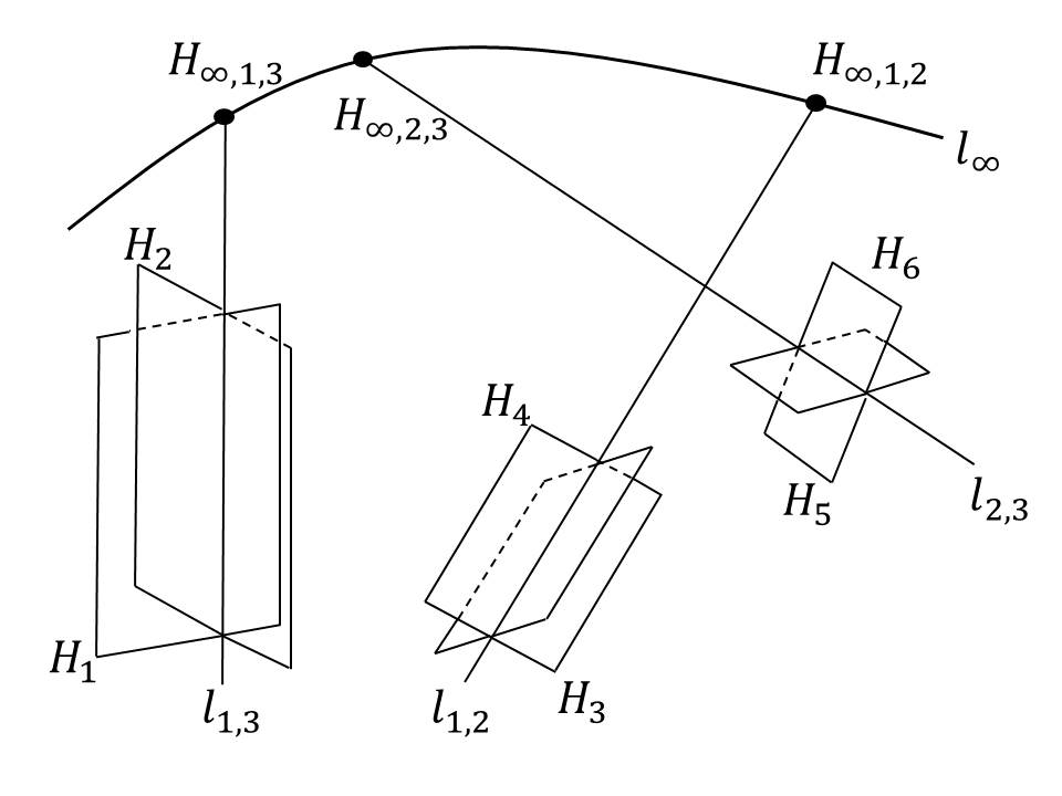 Figure 1