Exact Boson Sampling using Gaussian continuous variable measurements
A. P. Lund, S. Rahimi-Keshari, T. C. Ralph

TL;DR
This paper introduces a method for exact Boson Sampling using Gaussian continuous-variable measurements, demonstrating classical hardness for exact sampling, but not for approximate sampling, thus advancing quantum computational complexity understanding.
Contribution
It presents a novel device setup combining Fock states, linear interactions, and Gaussian measurements that achieves classically hard exact sampling, extending Boson Sampling concepts.
Findings
Exact sampling is classically hard for the proposed device.
Gaussian measurements do not imply hardness for approximate sampling.
The paper discusses conditions needed for approximate sampling hardness.
Abstract
BosonSampling is a quantum mechanical task involving Fock basis state preparation and detection and evolution using only linear interactions. A classical algorithm for producing samples from this quantum task cannot be efficient unless the polynomial hierarchy of complexity classes collapses, a situation believe to be highly implausible. We present method for constructing a device which uses Fock state preparations, linear interactions and Gaussian continuous-variable measurements for which one can show exact sampling would be hard for a classical algorithm in the same way as Boson Sampling. The detection events used from this arrangement does not allow a similar conclusion for the classical hardness of approximate sampling to be drawn. We discuss the details of this result outlining some specific properties that approximate sampling hardness requires.
Click any figure to enlarge with its caption.
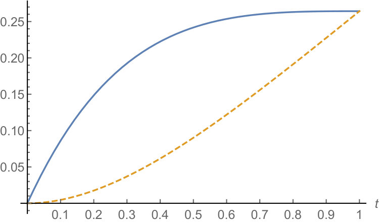 Figure 1
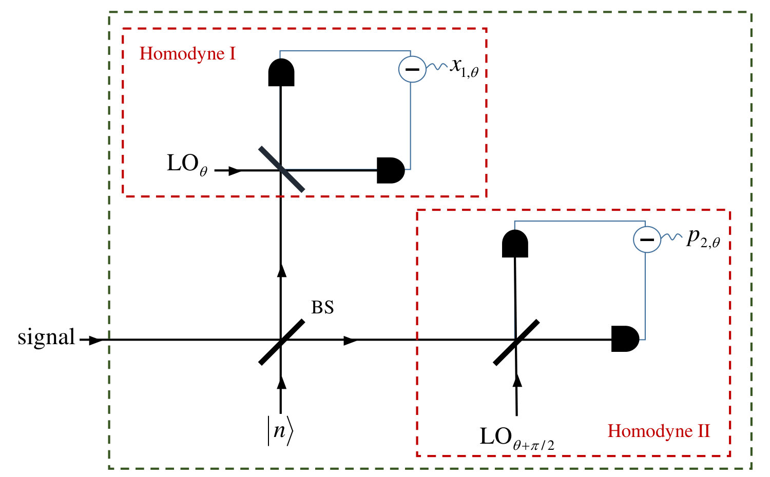 Figure 2
 Figure 2
Peer Reviews
No public reviews on file for this paper yet. If you reviewed it on a platform where reviews are public (OpenReview, ICLR, NeurIPS, ICML), you can paste yours below so the community can read it here.
Videos
No videos yet. Explain this paper in a talk, walkthrough, or lecture? Add one.
\newclass\SampP
SampP \newclass\SampBQPSampBQP \newclass\IQPIQP \newclass\BosonSamplingBosonSampling \newclass\FBPPFBPP
Exact BosonSampling using Gaussian continuous variable measurements
A. P. Lund
Centre for Quantum Computation and Communications Technology, School of Mathematics and Physics, The University of Queensland, St Lucia, Queensland, 4072, Australia
S. Rahimi-Keshari
School of Physics, Institute for Research in Fundamental Sciences (IPM), P.O.Box 19395-5531, Tehran, Iran
Centre for Quantum Computation and Communications Technology, School of Mathematics and Physics, The University of Queensland, St Lucia, Queensland, 4072, Australia
T. C. Ralph
Centre for Quantum Computation and Communications Technology, School of Mathematics and Physics, The University of Queensland, St Lucia, Queensland, 4072, Australia
Abstract
is a quantum mechanical task involving Fock basis state preparation and detection and evolution using only linear interactions. A classical algorithm for producing samples from this quantum task cannot be efficient unless the polynomial hierarchy of complexity classes collapses, a situation believe to be highly implausible. We present method for constructing a device which uses Fock state preparations, linear interactions and Gaussian continuous-variable measurements for which one can show exact sampling would be hard for a classical algorithm in the same way as Boson Sampling. The detection events used from this arrangement does not allow a similar conclusion for the classical hardness of approximate sampling to be drawn. We discuss the details of this result outlining some specific properties that approximate sampling hardness requires.
I Introduction
is the task of producing statistical samples from Fock basis measurements of a bosonic -mode linear scattering network with an input consisting of modes prepared with a single boson and the remaining modes prepared in the vacuum state. This task, whilst not universal for quantum computing, has been shown to not be efficiently computable by any classical algorithm (or the polynomial hierarchy of complexity classes collapses which is believe to be extremely unlikely) AA . However, a quantum implementation is efficient as one merely needs to build the scattering device as described within a sufficiently small error budget. This is many orders of magnitude easier than the construction of a fully universal quantum computer, but is still a challenge for current technology.
Attempts have been made to identify scenarios where the proof of classical hardness of can be used or adapted to other sampling problems. One particular scenario that is of experimental interest is in the use of continuous variable (CV) Gaussian states or measurements. For another restricted computational model based on sampling from qubit circuits involving commuting coherent rotations it has been shown that CV variants are hard to simulate classically Douce17 . It is known that for linear networks with Gaussian state inputs and Gaussian measurements it is efficient for classical algorithms to not only produce samples but compute the entire output distribution Bartlett03 . Never-the-less it has been shown that a hybrid approach which involves linear networks with input two-mode squeezed vacuum states and Fock basis detection has a similar classical hardness proof to the original problem Lund2014 . There is also evidence for the classical hardness of a more general construction involving squeezed-vacuum inputs, linear optics and Fock basis detection Rahimi2015 ; Ham2016 . The question this paper addresses is the reverse situation, Fock state inputs to linear networks and homodyne detection.
An important aspect of the hardness proof for is that the output probability distribution contains probabilities which are proportional to matrix permanents from sub-matricies of the matrix describing the linear scattering network. A matrix permanent is a quantity which is computed like a matrix determinant without the alternating addition and subtraction. In fact, when sampling with Fock state inputs and detection, all detection probabilities are proportional to sub-matricies derived from the linear scattering network Scheel04 . This special situation, given two plausible conjectures hold, allows for the hardness proof of “approximate” sampling to be shown AA . This is because an allowed error budget’s effect can be spread over all detection events provided the linear network appears randomly distributed.
Here we show that using single-photon input states and a particular Gaussian measurement one can extract sub-matrix permanents to within an exponentially small error. Therefore one can show that exact sampling from this distribution is hard. It is not necessarily the case that approximate sampling is still hard and we discuss this in relation to our construction.
In section II we present some of the background behind the hardness arguments for . Then in section III we present the CV-n detector model using a Fock state input with CV measurements. In section IV we will then describe exact sampling using the CV-1 model and the technical details involved in showing the hardness of computing samples from the CV output distribution. Finally we will discuss the issues preventing the hardness result from being used in this model to make definitive conclusions about the hardness or not of approximate sampling.
II Classical hardness of
A problem in the class is one where the statistical samples can be generated by an mode linear interaction between singly occupied bosonic modes (and bosonic vacua) which is subsequently detected in the Fock basis. is either inefficient using classical computational resources (not in ), or the “polynomial hierarchy” of complexity classes collapses to the third level, a situation believe to be implausible. It is not our goal to present in full the background and subsequent arguments towards the truth of this statement as this has been done elsewhere AA . We will, however, outline some of the key aspects used in this paper that are needed to understanding what is required for the proof presented in AA to hold.
II.1 Polynomial hierarchy
The polynomial hierarchy of complexity classes is a nested structure defined by the use of oracles. An oracle is essentially an assumption on the resources available to an algorithm which can greatly assist in proving statements in computational complexity. The hierarchy has a complex definition and we will concentrate on a simplified version.
The class is the set of decision (’yes’/’no’) problems whose satisfying input can be verified efficiently. This defines the first level of the polynomial hierarchy. The second level is then the class with access to an oracle from the first level. Subsequent levels are defined by continuing this recursion, e.g. the third level is the class with access to an oracle from the second level.
This structure has a strong connection to similarly defined hierarchies within number theory and set theory. In those cases each level of the hierarchy is strictly larger than lower levels. If two levels were to coincide, then the addition of levels stops growing the hierarchy is said to collapse. In terms of the computational complexity structure, a collapse of the hierarchy to the first level means that or that problems can be efficiently solved deterministically a situation believed to be highly implausible. A collapse to the second level would mean which is the same statement relative to an oracle. Being relative to the oracle means that the statement is slightly more plausible, but it is still believed to be not possible. The prevailing belief is that the polynomial hierarchy does not collapse to any level and this is the assumption on which the hardness of can be proven.
II.2 Stockmeyer’s approximate counting algorithm
Critical to the hardness proof of is the use of Stockmeyer’s approximate counting algorithm Stockmeyer1983 . This algorithm computes estimates of a quantity defined as
[TABLE]
where is a boolean function from length bitstrings onto a single bit. In other words is the number of inputs that result in an output of , a set we will call . The computed estimate of this quantity is multiplicative, which means the estimate of that the algorithm produces is satisfying
[TABLE]
where and for Stockmeyer’s algorithm is lower bounded by .
Stockmeyer’s algorithm computes the estimate by finding the smallest output with no collisions for a randomly chosen hash functions on . That is, choose randomly a function (for ) and if there exists no elements such that (a hash collision) then we have made an upper bounded estimate on the size of of .
Here we can see the elements which make up this algorithm: the estimate of size is multiplicative, it requires finding hash collisions, which is an problem, and involves random choices. This results in Stockmeyer’s algorithm being contained within a class (if the function is efficiently computable). The superscript notation describes access to an oracle, which in the case of Sockmeyer’s algorithm is used to find hash collisions. means the algorithm proceeds by making random (probabilistic) choices with a probability of success at least . The prefix ’F’ is used to describe the output from this algorithm, which is a number (function) rather than a decision or ’yes’/’no’ output. This is therefore not an algorithm one would expect to be efficiently computable when realistically implemented. But it is used here to establish if a problem lives within the “polynomial” hierarchy of complexity classes. In this case, this algorithm lives within the third level as Sip ; Laut .
This algorithm is used to make multiplicative estimations of the underlying probabilities of a distribution from samples of the distribution. In the model of classical computation, unlike quantum mechanical models, there is no inherent randomness. Randomness is introduced by external means and can be regarded as an input to the algorithm. If the function above represent a sampling algorithm for a two-outcome distribution, then it can be thought of as converting input random bits distributed uniformly into samples of the desired probability distribution. One can then estimate the probability of the outcome by counting how many inputs produce the outcome relative to the total number of possible inputs. This would mean dividing the estimate by which will also produce a multiplicative estimate even though it has been divided by an exponentially increasing factor.
A polynomial hierarchy collapse is triggered if is efficient to compute and the probability it produces samples from is a quantity for which multiplicative estimation is known to be outside the third level of the polynomial hierarchy.
II.3 Multiplicative and additive errors
Producing approximations within multiplicative errors is particularly powerful. It is more natural to consider the case of additive errors. An additive estimate of would be one satisfying
[TABLE]
This kind of estimation will arise from more natural models of errors within a computation. For example, the function above most likely admits errors which are of an additive nature and hence the estimations performed using this noisy model will also be additive. Only in the case of admitting exactly zero noise to , or in the sampling case a situation called “exact sampling”, can one generate a multiplicative estimation.
The crucial outcome of AA is that the polynomial hierarchy collapse can be shown to occur in even with a given level of total variation distance between the ideal and actual distributions. The total variation distance is an additive quantity and will generate additive errors in estimates. But as the probabilities in tend to decrease to zero exponentially, the introduction of additive errors will overwhelm the magnitude of the quantity being estimated. The trick of AA is to use the structure of the probabilities in to encode the estimated quantity within an exponentially large set of possible outcomes in a way that without knowledge of where the problem is encoded, looks like a Haar-random unitary matrix (i.e. the choice is hidden from the implementation). This means that the additive estimate generated will have bounds determined by the average case which turns out to be sufficient to additively estimate matrix permanents. Using this estimate it is then possible to trigger a polynomial hierarchy collapse to the third level, given that two plausible conjectures about the nature of estimating permanents of Gaussian random matrices hold true.
III The detector
We will now describe our continuous-variable detection model and how we use it to construct a probability distribution which can be used in the arguments of AA . The model is based on a measurement device for measuring in the displaced number state basis, which we refer to it as CV-n measurement, and two variations of this measurement, phase-randomised CV-n (PRCV-n) and discretised-phase-randomised CV-n (DPRCV-n). Only a brief outline of the model is presented here. The details of this calculation are given in Appendix A.
As depicted in Fig. 1, the measurement device works as follows. The input signal is overlapped on a 50:50 beamsplitter with a number state , and the outputs of the beamsplitter are measured by two conjugate homodyne detections whose local oscillators have phase difference. As shown in Appendix A, the POVM elements of this measurement are
[TABLE]
The two real numbers , form the results of a simultaneous measurement of two orthogonal quadratures. Notice that for , CV-0, we have heterodyne measurement.
Phase-randomised CV-n (PRCV-n). If the phase of the local oscillators is randomised, while the relative phase is fixed, we have PRCV-n measurement. As discussed in Appendix A, the outcome of this measurement is a single non-negative parameter with the corresponding POVM element
[TABLE]
with being the generalized Laguerre polynomials. Though this measurement has less information, we will concentrate on it as we are only interested in events where and having the POVM diagonal in the Fock basis greatly simplifies many calculations.
Discretized-phase-randomised CV-1 (DPRCV-1). The measurement model outputs continuous variables (i.e. ) and hence these POVMs are describing probability densities. To be able to use the methods of AA to make some definitive statement about computational hardness, one must work in probabilities and not probability densities. Hence, we will utilize the discretized version of the phase-randomized CV-1 (DPRCV-1) measurement through its ability to distinguish between the single-photon state and other number states. We divide the range of for the POVM elements in Eq. (5) for , to two parts which represents the smallest discrete region and which represents all the others. Thus, we have two POVM elements for each interval:
[TABLE]
where
[TABLE]
with being the lower incomplete Gamma function. As this is a two-outcome measurement and each of the elements is bounded above by the POVM for all other outcomes can then be written
[TABLE]
The POVM element in Eq. (6) can be expanded in a power series as
[TABLE]
Therefore, if is small such that , the POVM element associated with detecting is
[TABLE]
It is this form of the POVM which allows for a measurement that distinguishes a single photon Fock state from the remainder of the Hilbert space.
To demonstrate what this measurement is detecting consider the case of an input states being either or . Then when detecting the single photon state (and for any value of ),
[TABLE]
can be thought of as the efficiency of the detector. Also
[TABLE]
can be thought as the dark count probability. Fig. 2 compares these two quantities.
IV Boson sampling
We now consider the problem of sampling from the output probability distribution of a linear-optical network (LON) using CV-1, PRCV-1, and DPRCV-1 measurements (where the ancillary Fock state is ) introduced in the previous section. We first derive the output probability distribution for each measurement scheme, and then discuss the complexity of sampling from the probability distribution.
IV.1 Probability distributions
In this setup, the input state to the LON is
[TABLE]
Each output mode is measured by a CV-1 measurement; hence, the overall POVM elements are
[TABLE]
where . As shown in Fig. 3, this setup is equivalent to injecting single photons into a larger network and performing homodyne measurements at the output, i.e., boson sampling with homodyne measurements.
Therefore, the output probability density is given by
[TABLE]
Here is the unitary operation associated with the LON, and is the multimode Fock state. As a LON preserves the number of photons, the sum is restricted to ’s which satisfy .
We have Scheel04
[TABLE]
which is the permanent of an submatrix of the unitary matrix of LON, that is corresponding to the first rows and columns with multiplicity of . The unitary matrix is defined through the relation
[TABLE]
where and are modal creation operators for output and input , respectively. Also, using the expression for in Cah-Glau , one can simply verify that
[TABLE]
By using these relations, the output probability density (15) becomes
[TABLE]
From this expression we can see that if , the probability density is zero unless .
We define as a -tuple whose elements are either zero or one and the number of ones is , and define a vector of length whose element are given by , i.e., it has zero elements corresponding to . Using these notations, we can see that
[TABLE]
where the product is over nonzero elements of . This implies that if of ’s are zero, the probability density is proportional to the absolute value square of permanent of a submatix of . For example, for
[TABLE]
If we use PRCV-1 measurements at the output of LON, using the POVM (68), the output probability density is given by
[TABLE]
where and . Defining similar to , we have
[TABLE]
For DPRCV-1 measurements at the output, the probability of detecting outcome , that is, clicks within interval and clicks within , using Eq. (7), is given by
[TABLE]
If is very small, this probability can be expanded to leading order in a powers of as
[TABLE]
where are -tuples whose elements are equal to except one 0 and one 1 are interchanged.
Notice that the probability distribution (23) corresponding to DPRCV-1 measurements is coarse-grained version of probability density (21), and that itself is phase randomised version of (18). Therefore, if exact sampling from the probability distribution (23) is classically hard, exact sampling from the other probability distributions must be classically hard as well. In the following two subsections we discuss exact and approximate sampling from the probability distribution (23).
IV.2 Exact boson sampling
To leading order in , Eq. (24) give a distribution for which hardness of exact sampling can be determined as we shall show in this section. Merely setting the terms to zero results in a probability
[TABLE]
A probability of this form does not pose any problems for the argument of hardness in exact sampling. However, it is important to consider higher order terms as exact sampling allows for sampling using any matrix even those with vanishingly small permanents. For example, one could consider the case where the permanent but the unwanted higher order terms have . Furthermore, as defines a probability distribution over all (i.e. the distribution) we have
[TABLE]
This means that, using Eq. (24), the probability can be written as
[TABLE]
where is an “error” over the desired probability. Unfortunately contributes to the probability in an additive sense. However, as we have used the upper bound on the matrix permanents that contribute to we know that this bound is independent of . So if we choose to be a small constant, we need to quadratically vary to achieve that constant. Furthermore, with constant , the sizes of sub-matrix permanents that can be estimated must be lower bounded with a bound that depends on .
To make this more explicit consider the case where . If we used the approximate counting algorithm using from Eq. (27) then we would have an estimate which satisfies
[TABLE]
where is the multiplicative error factor from the estimation. We can also write
[TABLE]
and using
[TABLE]
Now if (arbitrarily, could be any constant less than 1), we have
[TABLE]
where we now have a multiplicative error estimate with error .
The #P-hardness of approximating (Theorem 28 from AA ) where is an matrix, requires a choice of that is polynomially dependent on . This will be achieved here if the extra term maintains a polynomial scaling.
At this point, we consider the origin of the added error term to argue how must scale in terms of . All of the schemes described in Section III depend on a continuous output parameter based on the CV-1 style measurement. However, any experimental realisation will output values to within some precision. One particular way to do this, with a connection to discrete computational outputs is to consider a discretisation of the results into -bit integers. The outcomes from PRCV-1 are non-negative, so in this case consider -bit non-negative integers. is unbounded for large values, but in our scheme we are only interested in small values so we can choose an arbitrary fixed boundary above which all values are assigned the same bitstring output. With these requirements, results can be partitioned into regions such that the largest result corresponds to all outcomes above some fixed value, say . In the simplest case, if then we would have the one bit binary string with ‘[math]’ representing all results of the continuous value between [math] and and the binary string ‘’ representing values greater than . Increasing and continuing this division of the results, we find that the range of values covered by equal size partitions of the values between [math] and we have . It is the scaling in , and not , that is required to be considered when analysing the complexity of the problems modelled on this device.
We will proceed with the analysis below assuming this simple partitioning of the values of . It should be noted that other discretisation strategies can be considered. For example, a change of the discretisation thresholds such that smaller regions around zero can be considered by using a common technique called “companding”. However, one must be careful here not to sacrifice too much probability by having the zero region scale super-exponentially. Any scaling which results in the region at zero scaling as is sufficient for the exact sampling argument below. This is due to the nature of the Stockmeyer approximate counting algorithm utilized in AA. As these strategies do not change the complexity hardness result we present, we will not consider them further in this paper.
Now we will return to considering the error term . This quantity, as stated above, scales as . But in the number of bits used for discretisation it will scale as as . To achieve a scaling of a scaling in of would counteract the error leaving a overhead.
So our procedure will achieve a multiplicative estimate with a very quickly decaying lower bound on the matrix permanents that can estimate. But what actually determines the choice of the lower bound that is permitted? The proof of the #P-hardness for approximating proceeds in AA by using this estimation polynomially many times to compute given that was a zero-one matrix. As part of the proof one needs to use the estimation procedure in a binary search towards a matrix whose permanent is zero and the procedure stops when sufficient precision has been achieved to determine the permanent of the zero-one matrix, as it must be an integer value. Introducing a lower bound on the permanents for which the estimation is valid would have to be compatible with this final precision.
Never-the-less, in the hardness proof for approximate , it is assumed that the input matrices have matrix elements that have a Gaussian distribution. If one is to accept the conjectures of AA , then there is a low probability of randomly having near zero. Specifically, using the words from AA :
…if is Gaussian then …a fraction of [’s] probability mass is greater than in absolute value, being the standard deviation.
Using this we could choose the lower bound of to scale as . However, we have written the bound for our construction in terms of the submatrix of the unitary matrix . Following the embedding procedure from AA this reduces the size of by a factor involving the matrix norm . Therefore the probability reduces by a factor of as (the number of input photons) is a proxy for the problem input size (i.e. the matrix ) which must be efficiently represented in . This results in a scaling of . In terms of the discretisation bits the scaling is where the in this scaling is from the polynomial which bounds . So a polynomial scaling in the size of the discretisation allows for approximation of permanents which are highly probable when using an approximate algorithm. This argument shows that the exact sampling problem presented here, which permits multiplicative permanent estimation with permanents with an exponentially decreasing lower bound, must also be hard to compute with classical resources.
IV.3 Approximate sampling
The arguments just made do not permit one to continue the hardness argument through to the case of approximate sampling as was done in AA for the CV distributions we have constructed above. The reason is quite simple, only an exponentially small subset of events (i.e. detections near the origin) are used to make the exact sampling argument. Conversely, for the same reason, one also cannot definitively conclude that approximate sampling from this distribution is an efficient classical task.
The approximate sampling criterion for this CV distribution would be
[TABLE]
where is the probability density for our distribution of CV events from the device described above and is the computable approximation. The event used for sampling above is the set of , where ’s are around a ball of radius around the origin. Hence all of this error could potentially be concentrated on our event. This would dominate any exponential pre-factors of the matrix permanent in the probability exponentially reducing the signal that is being fed into the approximate counting algorithm.
Approximate sampling is shown in AA by potentially utilising all possible (or more precisely the collision-free subspace of) events to perform the approximate counting. The algorithm cannot know which event is being probed, so a concentrate of error as described above would result in the approximate sampling algorithm being an exact sampling algorithm for almost all results.
So what is required in the CV case is more events. To show classical hardness for this distribution, one needs to argue that events away from the origin are also #P-hard when used exactly. This is difficult for this construction as these events do not reduce to Fock basis measurements under any approximation. Also, there must be combinatorially enough events so that the approximate sampling error can be considered low enough on average over all the events so that hardness is maintained. Even if this specific criterion cannot be met, this does not mean that the distribution is efficient for a classical computation. To show classical efficiency, either a constructive proof demonstrating efficiency (e.g. the methodology used in SRK16-suff ) or some other proof technique ruling out classical hardness would be required.
V Conclusion
We have constructed a continuous variable measurement model we call CV-n which measures in a displaced number state basis. The measurement model can be achieved by mixing a photon state with the input on a 50:50 beam splitter then making homodyne measurements on the output. We have shown how a Fock basis state measurement can be approximately achieved using this measurement utilising those cases when the homodyne measurement outcomes are simultaneously small.
We then showed that this measurement model is compatible with the exact problem, a computing task that has been shown to be inefficient for any classical device to simulate. We have discussed how this model as presented here is not compatible with approximate as the detection events utilised, when compared with the whole event space, is too small.
Acknowledgements
This work was supported by the Australian Research Council Centre of Excellence for Quantum Computation and Communications Technology (Project No. CE110001027).
Appendix A CV-n measurement: Continuous variable measurement in the displaced number state
In this appendix we obtain the POVM elements of the CV-n measurement; see Fig. 1. The POVM elements of this measurement are of this form
[TABLE]
where and are the outcomes of the fist and the second homodyne measurements, respectively, and is the normalization constant such that .
The POVM elements of the first homodyne measurement are
[TABLE]
where
[TABLE]
Notice that is an infinitely squeezed vacuum state, and can be written as
[TABLE]
with being the squeezing operator and being the vacuum state.
For the second homodyne measurement we have
[TABLE]
where
[TABLE]
Similarly, we have
[TABLE]
Now using Eqs. (34) and (37), in Eq. (33) is given by
[TABLE]
where is the normalization constant. Using the following relations for the 50:50 beamsplitter
[TABLE]
the expression in Eq. (40) becomes
[TABLE]
where
[TABLE]
and is the displacement operator. Thus, Eq. (40) becomes
[TABLE]
Using
[TABLE]
we can write Eq. (46) as
[TABLE]
It can be shown that
[TABLE]
where
[TABLE]
and the second equality can be seen using this expression
[TABLE]
with being the generalized Laguerre polynomials.
By substituting from Eq. (51) into Eq. (50), we get
[TABLE]
As this state must be normalized in the limit of , it is straightforward to see that
[TABLE]
As , we now have
[TABLE]
where
[TABLE]
Therefore, POVM elements of the CV-n measurement are
[TABLE]
Notice that, it can be simply checked that
[TABLE]
A.1 Phase randomized CV-n measurement
If the phase of the local oscillator is randomized, with the relative phase being fixed, we have
[TABLE]
where
[TABLE]
The matrix elements of this operator in the Fock basis are
[TABLE]
Therefore, the POVM elements of the phase randomized measurement are given by
[TABLE]
It can be simply verified that
[TABLE]
For , using
[TABLE]
we have
[TABLE]
so the POVM elements (68) becomes
[TABLE]
Notice that
[TABLE]
as expected.
The reference list from the paper itself. Each links out to its DOI / PubMed record.
- 1(1) S. Aaronson and A. Arkhipov, Theory Comput. 9 , 143 (2013).
- 2(2) S. D. Bartlett, B. C. Sanders, S. L. Braunstein, K. Nemoto, Phys. Rev. Lett. 88 , 097904 (2002); S. D. Bartlett and B. C. Sanders. Journal of Modern Optics, 50 , 2331–2340 (2003).
- 3(3) A. P. Lund, A. Laing, S. Rahimi-Keshari, T. Rudolph, J. L. O’Brien and T. C. Ralph, Phys. Rev. Lett. 113 , 100502 (2014).
- 4(4) S. Rahimi-Keshari, A. P. Lund and T. C. Ralph, Phys. Rev. Lett. 114 , 060501 (2015).
- 5(5) C. S. Hamilton, R. Kruse, L. Sansoni, S. Barkhofen, C. Silberhorn, I. Jex, ar Xiv:1612.01199 [quant-ph].
- 6(6) T. Douce, D. Markham, E. Kashefi, E. Diamanti, T. Coudreau, P. Milman, P. van Loock, and G. Ferrini Phys. Rev. Lett. 118 , 070503 (2017).
- 7(7) Stefan Scheel, quant-ph/0406127 (2004).
- 8(8) L .J. Stockmeyer. The complexity of approximate counting. In Proc. ACM STOC , pp 118–126 (1983).