Three Asymptotic Regimes for Ranking and Selection with General Sample Distributions
Jing Dong, Yi Zhu

TL;DR
This paper investigates three asymptotic regimes for ranking and selection problems with general distributions, establishing their validity, efficiency, and interconnections, and comparing algorithm performances in these regimes.
Contribution
It introduces and analyzes three novel asymptotic regimes for R&S with general distributions, providing theoretical validation and performance comparisons.
Findings
Asymptotic regimes are valid and efficient for R&S.
Connections among different regimes are characterized.
Pre-limit algorithm performances are compared.
Abstract
In this paper, we study three asymptotic regimes that can be applied to ranking and selection (R&S) problems with general sample distributions. These asymptotic regimes are constructed by sending particular problem parameters (probability of incorrect selection, smallest difference in system performance that we deem worth detecting) to zero. We establish asymptotic validity and efficiency of the corresponding R&S procedures in each regime. We also analyze the connection among different regimes and compare the pre-limit performances of corresponding algorithms.
Click any figure to enlarge with its caption.
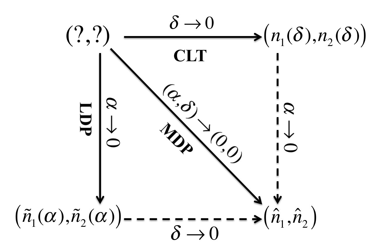 Figure 1
| Regime | Probability of Incorrect Selection | |
|---|---|---|
| CLT Regime | ||
| LD Regime | ||
| MD Regime |
| Regime | Probability of Incorrect Selection | |
|---|---|---|
| CLT Regime | ||
| LD Regime | ||
| MD Regime |
Peer Reviews
No public reviews on file for this paper yet. If you reviewed it on a platform where reviews are public (OpenReview, ICLR, NeurIPS, ICML), you can paste yours below so the community can read it here.
Videos
No videos yet. Explain this paper in a talk, walkthrough, or lecture? Add one.
Taxonomy
TopicsGame Theory and Voting Systems · Auction Theory and Applications · Consumer Market Behavior and Pricing
Three Asymptotic Regimes for Ranking and Selection with General Sample Distributions
Jing Dong, Yi Zhu
Abstract
In this paper, we study three asymptotic regimes that can be applied to ranking and selection (R&S) problems with general sample distributions. These asymptotic regimes are constructed by sending particular problem parameters (probability of incorrect selection, smallest difference in system performance that we deem worth detecting) to zero. We establish asymptotic validity and efficiency of the corresponding R&S procedures in each regime. We also analyze the connection among different regimes and compare the pre-limit performances of corresponding algorithms.
1 Introduction
Ranking and selection (R&S) refers to the statistical procedure to select the simulated systems with the best performance (largest or smallest mean) among a finite number of alternatives with high probability. Most of the existing procedures are constructed under the assumption that the samples follow a Gaussian distribution or some other rather restricted class of distributions (e.g. sub-Gaussian, bounded support) to gain control over the probability of correct selection. When these assumptions are violated, the desired performance can only be guaranteed in an asymptotic sense.
Asymptotic analysis is achieved by sending the sample size to infinity. However, simply sending the sample size to infinity will not convey any meaningful information. By law of large numbers, it simply implies that the probability of correct selection will converge to one. To define the asymptotic regimes in a proper and meaningful way, we consider two parameters that characterize the “difficulty” of the problem: 1) the difference between the best system and the second best system, which we denote as ; 2) the probability of incorrect selection (PIS), which we denote as . Under the indifference zone formulation, denotes the smallest difference in system performance that we deem worth detecting. Thus, is also known as the indifference-zone parameter. As either one of these parameters gets smaller, it requires more samples to achieve the desired performance.
In this paper, we study asymptotic regimes that can be applied for R&S problems with general sample distributions. The first limiting regime is called the central limit theorem regime, which is derived by sending to zero. The second limiting regime is called the large deviation regime, which is derived by sending to zero. The third limiting regime is called the moderate deviation regime, which is derived by sending to zero at an appropriate rate. We present the theoretical foundation of each limiting regime and develop sequential stopping procedures for problems with unknown variance.
The central limit theorem regime has been applied in the R&S literature, mostly under the the indifference zone formulation. [10] defined that an indifference zone procedure is asymptotically consistent if . [11] propose a sequential stopping procedure for R&S problems with unknown variance and show that their algorithm is asymptotically consistent. [9] develop a fully sequential selection procedure for steady-state simulation that is shown to be asymptotically consistent. This limiting regime has also been used to establish the asymptotic validity of sequential stopping procedures to construct fixed-width confidence intervals [7]. The limit is achieved by sending the width of the confidence interval to zero. We will provide more details about this limiting regime in §2.1.
The large deviation regime has been applied in the ordinal optimization literature. The appealing fact is that while the width of the confidence interval decreases at rate (due to the central limit theorem), the PIS actually decays exponentially fast in (due to the large deviation theory) [3]. Results from this limiting regime, in particular, the large deviation rate function of the PIS, has been applied to find the optimal budget allocation rules, i.e. to minimize PIS under a fixed budget (see for example [5], [13] and [8]). The large deviation type of upper bound on the probability of incorrect selection has also been applied in the multi-arm bandit literature [2]. Compared to the R&S literature, the key performance measure for the multi-arm bandit literature is the regret, which measures the cumulative opportunity cost of not knowing the optimal system. Two of the well-known sampling strategies in this literature is the upper confidence bound strategy and the Thompson sampling. Both are shown to achieve an regret bound, under the assumption that we have access to the large deviation rate function or an upper bound of the rate function in closed form. This assumption imposes constrains on the type of sample distributions we can work with. We will survey more details about this limiting regime in §2.2.
To the best of our knowledge, the moderate deviation regime studied in this paper has not been applied in the R&S or the ordinal optimization literature, though the moderate deviation theory is well-studied in the applied probability literature [4]. As we shall explain in subsequent development (§2.3), this asymptotic regime tends to strike a balance between the central limit theorem regime and the large deviation regime.
2 The Three Asymptotic Regimes
To demonstrate the basic ideas, we restrict our discussion to the comparison between two systems. To formalize the asymptotic analysis, we first define a suitable sequence of distributions. Let and be two random variables with the same mean and potentially different variance, and , respectively. We define , indexed by , as a sequence of random variables with cumulative distribution function , i.e. . In particular, . We denote , , as i.i.d. copies of , and , , as i.i.d. copies of . Let
[TABLE]
denote the sample means of and . We also denote the sample variances as
[TABLE]
Our goal is to select the system with the largest mean value when comparing and . In particular, if we draw samples from and samples from , and select the system with the largest sample mean, then
[TABLE]
Remark 1**.**
Other definitions of the sequence of random variables may also work. In general, we need to assume that the variances of ’s do not depend on .
Recall that denotes the required level of the PIS, and denotes the difference in mean between the two systems ( and ). We consider the following three asymptotic regimes. i) Keep fixed and send to zero; ii) Keep fixed and send to zero; iii) Send both and to zero at an appropriate rate. We shall elaborate on each of these three regimes next.
2.1 The Central Limit Theorem Regime
In this limiting regime, we keep fixed and send to zero. We start with the known variance case. For fixed satisfying , we set the required sample sizes as
[TABLE]
where is the -th upper tail quantile of a standard normal distribution. We draw samples from system i, and pick the system with the largest mean. The following theorem establishes the asymptotic validity of this procedure.
Theorem 1**.**
Under the assumption that for ,
[TABLE]
Proof of Theorem 1.
We notice that
[TABLE]
The convergence follows by Central Limit Theorem. ∎
We next introduce some possible choices of the parameter ’s. i) If we are to minimize for each value of , then we set and . In this case
[TABLE]
ii) If we want to draw equal amount of samples from both systems, then we set , for . In this case
[TABLE]
iii) If we want to run the simulation without taking into account the information of the other system, then we can set, for example, . In this case
[TABLE]
When the variances are not known. We can apply the following sequential stopping procedure to decide the appropriate number of samples needed. In this paper, we will focus on the case of equal sample sizes only. We define the stopping time
[TABLE]
where is introduced to avoid early stopping. We keep sampling the two systems until the total sample variance over the sample size is smaller than , and then we pick the system with the largest sample mean. The following theorem establishes the asymptotic validity of the sequential stopping procedure.
Theorem 2**.**
Under the assumption that for ,
[TABLE]
Proof of Theorem 2.
For general , define , , and . We first notice that
[TABLE]
As and in as , where ,
[TABLE]
As is continuous and monotonically decreasing in [14],
[TABLE]
We next notice that
[TABLE]
As \frac{t}{\delta}(\bar{X}_{1}(t/\delta^{2})-\bar{X}_{2}^{0}(t/\delta^{2}))\Rightarrow\sqrt{\sigma_{2}^{2}+\sigma_{2}^{2}}B(t)\mbox{ in D[0,\infty)\delta\rightarrow 0}, using standard random time change and convergence together argument, we have
[TABLE]
in as . Thus,
[TABLE]
∎
Remark 2**.**
Alternatively, we can also set
[TABLE]
Then we can show that . The separation of the simulation of the two systems may become handy in parallelization.
2.2 The Large Deviation Regime
In this limiting regime, we keep fixed and send to zero. We impose light tail assumptions on the sample distribution.
Assumption 1**.**
There exists such that and .
We next introduce a few notations. Let and , i.e. the log moment generating functions. We also write which is known as the Fenchel-Legendre transformation of , for . Let and . It is well-known that is strictly convex and for . We also make the following assumption on the sample distribution
Assumption 2**.**
The interval .
We assume that ’s are known. For fixed with . We can interpret as the proportion of sampling budget allocated to system , . We denote . Then set the sample size
[TABLE]
We draw from system , , and pick the system with largest sample mean. The following theorem establishes the asymptotic validity, in a logarithmic sense, of the procedure.
Theorem 3**.**
[TABLE]
The proof of the theorem follows from the same line of analysis as in [5]. We shall only provide an outline here. Let . Then for . We also denote . Then the rate function of , is (Lemma 1 in [5])
[TABLE]
Then we have,
[TABLE]
Thus,
We next provide some special choices of ’s. i) If we want to minimize the sampling cost, then we pick that solves
[TABLE]
ii) If we want to draw equal amount of samples from the two systems, then we set . In this case
[TABLE]
iii) It is also possible to draw samples from each system without taking into account the information of the other system. For example, we can pick any and set
[TABLE]
However, in this case we “overshoot” the PIS. In particular, following the proof of Theorem 3, it is easy to check that
[TABLE]
In applications, the assumption that ’s are known is rather restrictive. When ’s are not known, estimating this function would in general be a more difficult task than estimating the means. Recently, [6] conduct an extensive analysis of this issue.
2.3 The Moderate Deviation Regime
In this regime, we send both and to zero at an appropriate rate. In particular, we consider a sequence of ’s, indexed by , satisfying that and as , and
[TABLE]
for some and , independent of .
We start by assuming that the variances are known. In this case, for fixed with , we set
[TABLE]
where . For , , we draw samples from system , and then choose the system with the largest sample mean. The following theorem establishes the asymptotic validity, in a logarithmic sense, of the procedure.
Theorem 4**.**
Under Assumption 1,
[TABLE]
Proof of Theorem 4.
Let , .
[TABLE]
Let , then
[TABLE]
By Gartner-Ellis theorem, satisfies a LDP with rate and rate function
[TABLE]
In particular,
[TABLE]
As , we have
[TABLE]
∎
We next provide some special choices of ’s. i) If we want to minimize the total sampling cost for each , then we pick for . In this case
[TABLE]
ii) When , we draw equal amount of samples from the two systems. In this case
[TABLE]
iii) It is also possible to draw samples from each system without taking into account the information of the other system. In particular, when ,
[TABLE]
When the variances are not known a priori, we introduce a sequential stopping procedure. In this paper, we shall focus on the case of equal sample sizes only. We also impose the following assumption on sample distribution (mainly for technical reasons).
Assumption 3**.**
There exist such that and .
We define the stopping time
[TABLE]
We keep sampling the two systems until the total sample variance over the sample size is smaller than , and then we pick the system with the largest sample mean. The following theorem establishes the asymptotic validity of the sequential stopping procedure.
Theorem 5**.**
Under Assumption 3,
[TABLE]
Remark 3**.**
Alternatively, we can also set
[TABLE]
Then following the same line of analysis as in the Proof of Theorem 5, we have
[TABLE]
The separation of the simulation of the two systems may become handy in parallelization.
2.3.1 Proof of Theorem 5
We first notice that as ,
[TABLE]
As the distribution of does not depend on . We shall drop the superscription when there is no confusion. Let for . As as , by Continuous Mapping Theorem
[TABLE]
We next establish an upper bound for for any small enough.
[TABLE]
for . Thus,
[TABLE]
where . By Gartner-Ellis Theorem, satisfies a LDP with rate function . Then we have
[TABLE]
and
[TABLE]
We denote for any . Then Let and . Then for any .
[TABLE]
We also notice that
[TABLE]
Thus,
[TABLE]
where the second inequality use the fact that is independent of , the third inequality follows from the proof of Theorem 4 and the fact that . Similarly,
[TABLE]
As and can be arbitrarily small, we have
[TABLE]
3 Comparison of the Three Asymptotic Regimes
The three asymptotic regimes are closely related to each other. Figure 1 provide an overview of their relationships. We’ve established the three solid arrows in the figure in §2. We next show the two dotted arrows for some special cases (Lemma 1 and Lemma 2).
Lemma 1**.**
The -th quantile of standard Normal distribution, , satisfies,
[TABLE]
Lemma 1 implies for small enough, and , we have , , and .
For the large deviation regime, when we impose equal sample sizes from the two systems, then we have . Let . We also define and . If we write , then .
Lemma 2**.**
For ,
[TABLE]
Lemma 2 implies that for small, , .
3.1 Pre-Limit Performance
We next provide some comments about the pre-limit performance, i.e. for fixed and . For simplicity of exposition, we shall restrict our discussion to the case of equal sample sizes.
In the Central Limit Theorem regime, when and are Gaussian random variables, we have . In general, the performance of “” depends on the “rate” of convergence of the central limit theorem. Assume that and is non-lattice. Let
[TABLE]
denote the skewness of . Skewness is a measure of asymmetry of a random variable about its mean. We also write
[TABLE]
as the Kurtosis of . Kurtosis measures the heaviness of the tail of a random variable. Let and denote the tail cumulative distribution function and the probability density function of a standard normal distribution. Using the Edgeworth expansion [12], we can show that
[TABLE]
We make the following observations. a) with . b) For distribution with large skewness or Kurtosis, the pre-limit PIS may be quite different from . A common practice to reduce the approximation error (improve the rate of convergence) is to use the Cornish-Fisher expansion [12] to refine the scaling parameter , but this would require us to know higher moments of the sample distributions.
For the large deviation regime, we first notice that, using Chernoff’s bound,
[TABLE]
To quantify how much smaller is, compared to , we refer to a refinement of the large deviation asymptotic approximation due to [1]. Assume that is steep on the right and is non-lattice. We denote . Then we can show that
[TABLE]
As , when is small enough, decays at rate approximately, which is slightly faster than . Therefore, sampling rules derived from the large deviation regime provide a guarantee on PIS but tend to over-sample in practical examples.
For the moderate deviation regime, we first notice that for fixed value of . Thus, we tend to sample more than “needed” when the central limit theorem regime works well. However, this also provides us with a safety buffer when the central limit theorem regime doesn’t work well.
3.2 Numerical Comparison
The following numerical experiments illustrate the pre-limit performance of the sampling rules derived from the three asymptotic regimes (Table 1 & 2). The probability of incorrect selection are calculated based independent experiments. In Table 1, we assume both systems have Exponential sample distributions. We observe that in this case, the CLT regime sampling rule achieves the desired probability of incorrect selection, but the other two regimes overshoot the probability of incorrect selection, i.e. . Table 2 illustrate an extreme example, where system 1 has constant output while system 2 has Bernoulli sample distribution with very small probability of success (highly skewed). There the CLT regime doesn’t achieve the desired probability of incorrect selection while the LD regime over-samples. We would also like to point out that among the three regimes, the LD regime is the only one that is guaranteed to have regardless of the sample distributions.
Appendix A Proofs
Proof of Lemma 1.
We first notice that As as , then
[TABLE]
Similarly,
[TABLE]
Thus,
[TABLE]
∎
Proof of Lemma 2.
Applying Taylor expansion, we have for
[TABLE]
Let . Then and
[TABLE]
We also notice that Thus, . The results then follows by noting that , and for . ∎
The reference list from the paper itself. Each links out to its DOI / PubMed record.
- 1[1] R.R. Bahadur and R.R. Rao. On deviations of the sample mean. Annals of Mathematical Statistics , 31(4):1015–1027, 1960.
- 2[2] S. Bubeck and N. Cesa-Bianchi. Regret analysis of stochastic and nonstochastic multi-armed bandit problems. Foundations and Trends in Machine Learning , 5(1):1–122, 2012.
- 3[3] L. Dai. Convergence properties of ordinal comparison in the simulation of discrete event dynamic systems. Journal of Optimization Theory and Applications , 91(2):363–388, 1996.
- 4[4] A. Dembo and O. Zeitouni. Large deviation techniques and applications . Springer, New York, 1998.
- 5[5] P. Glynn and S. Juneja. A large deviation perspective on ordinal optimization. In R.G. Ingalls, M.D. Rossetti, J.S. Smoth, and B.A. Peters, editors, Proceedings of the 2004 Winter Simulation Conference , pages 577–585, Piscataway, New Jersey, 2004. IEEE, inc.
- 6[6] P. Glynn and S. Juneja. Ordinal optimization - empirical large deviations rate estimators, and stochastic multi-armed bandits. Working paper, available at http://arxiv.org/pdf/1507.04564 v 1.pdf, 2015.
- 7[7] P. Glynn and W. Whitt. The asymptotic validity of sequential stopping rules for stochastic simulations. The Annals of Applied Probability , 2(1):180–198, 1992.
- 8[8] S.R. Hunter and R. Pasupathy. Optimal sampling laws for stochastically constrained simualtion optimization on finite sets. INFORMS Journal on Computing , 25(3):527–542, 2013.