Stability and $\ell^2$-gain Analysis of Adaptive Control Systems with Event-triggered Try-once-discard Protocols
Masashi Wakaiki

TL;DR
This paper develops stability and $ ext{l}^2$-gain analysis methods for adaptive control systems employing event-triggered try-once-discard protocols, ensuring practical stability and performance bounds.
Contribution
It introduces new stability conditions and $ ext{l}^2$-gain bounds for adaptive control systems with event-triggered measurement transmission protocols.
Findings
Provided sufficient conditions for practical stability.
Derived upper bounds on the $ ext{l}^2$-gain.
Applicable to gain-scheduling and switching controllers.
Abstract
This paper addresses the stability and -gain analysis of adaptive control systems with event-triggered try-once-discard protocols. At every sampling time, an event trigger evaluates an error between the current value and the last released value of each measurement and determines whether to transmit the measurements and which measurements to transmit, based on the try-once-discard protocol and given lower and upper thresholds. For gain-scheduling controllers and switching controllers that are adaptive to the maximum error of the measurements, we obtain sufficient conditions for the practical stability and upper bounds on the -gain of the closed-loop system.
Click any figure to enlarge with its caption.
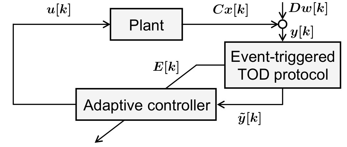 Figure 1
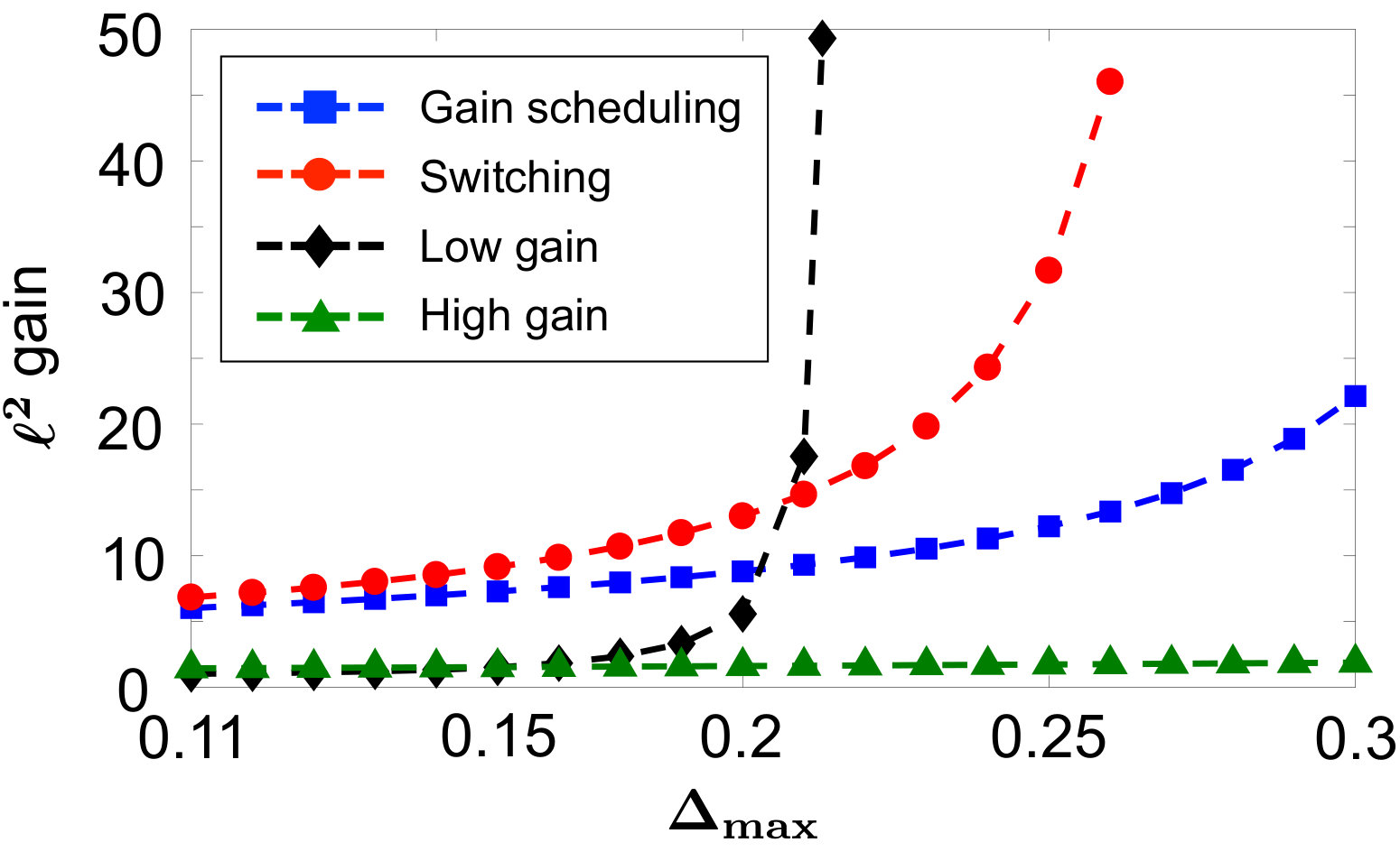 Figure 2
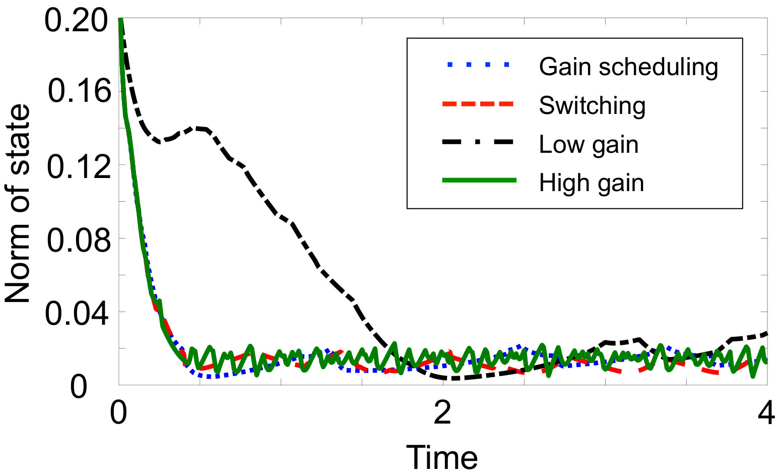 Figure 3
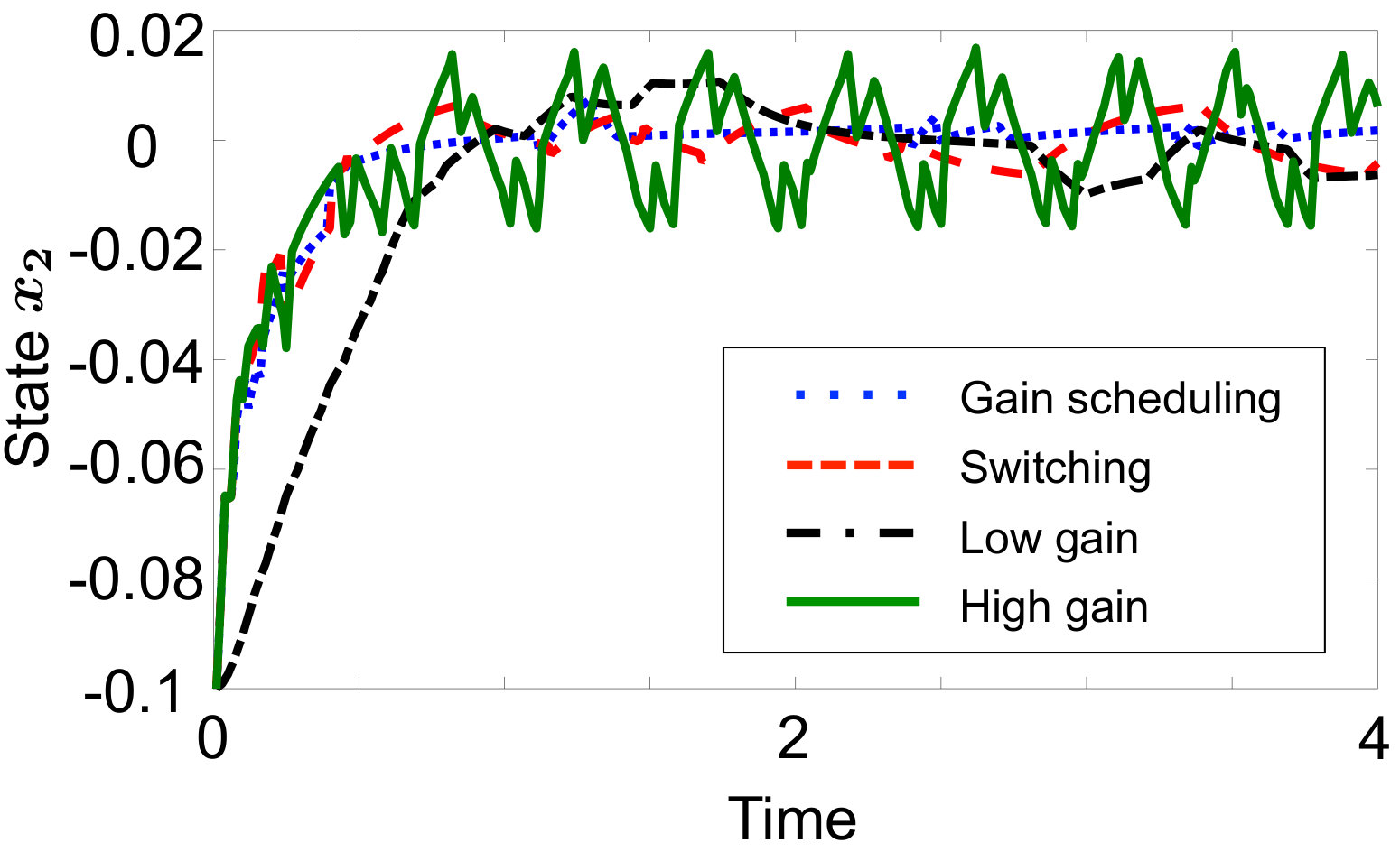 Figure 4
Peer Reviews
No public reviews on file for this paper yet. If you reviewed it on a platform where reviews are public (OpenReview, ICLR, NeurIPS, ICML), you can paste yours below so the community can read it here.
Videos
No videos yet. Explain this paper in a talk, walkthrough, or lecture? Add one.
Stability and -gain Analysis of Adaptive Control Systems with Event-triggered
Try-once-discard Protocols
Masashi Wakaiki
This work was supported by JSPS KAKENHI Grant Numbers JP17K14699. Masashi Wakaiki is with the Graduate School of System Informatics, Kobe University, 1-1 Rokkodai, Nada, Kobe, 657-8501, Japan (e-mail: [email protected]).
Abstract
This paper addresses the stability and -gain analysis of adaptive control systems with event-triggered try-once-discard protocols. At every sampling time, an event trigger evaluates an error between the current value and the last released value of each measurement and determines whether to transmit the measurements and which measurements to transmit, based on the try-once-discard protocol and given lower and upper thresholds. For gain-scheduling controllers and switching controllers that are adaptive to the maximum error of the measurements, we obtain sufficient conditions for the practical stability and upper bounds on the -gain of the closed-loop system.
Index Terms:
Stability of linear systems, Networked control systems, LMIs.
I Introduction
In standard sampled-data control, measurements are periodically transmitted to controllers. For this time-triggered control, many techniques of designing controllers have been developed during last decades such as the lifting approach [1, 2], the fast sample/fast hold approach [3], and the frequency response operator approach [4]. However, time-triggered control may lead to redundant transmissions, which waste energy and network resources.
As an alternative control paradigm, event-triggered control [5, 6] has been developed. In the event-triggered approach, transmission intervals are determined by a predefined condition on the measurements, and energy and network resources are used only if the measurements have to be transmitted. The effectiveness of event-triggered techniques has been illustrated, e.g., through security in networked control systems in [7, 8, 9] and an experiment of mobile robots in [10, 11], and there are many researches on the analysis and synthesis of event-triggered control as surveyed in [12, 13].
To avoid network congestion, medium access protocols such as the Round-Robin (RR) protocol and the Try-Once-Discard (TOD) protocol govern the access of nodes to networks. The RR protocol assigns transmissions to the nodes in a prefixed order. In contrast, the TOD protocol determines which nodes should transmit their data by evaluating the largest error between the current value and the last released value of the node signals; see [14, 15, 16, 17, 18] and references therein for control methods based on the TOD protocol.
In this paper, we study the stability and -gain analysis of adaptive control systems with event-triggered TOD protocols. As the periodic event-triggered control proposed in [19, 20], an event trigger periodically evaluates errors between the current values and the last released values of the measurements and determine whether to transmit the measurements and which measurements to transmit, based on the TOD protocol and given lower and upper thresholds.
In the usual event-triggered control, e.g., of [5, 6, 19, 20, 21, 22, 23], the controller knows that if it does not receive the measurements, then the errors between the current values and the last released values of the measurements are smaller than a prefixed threshold. In addition to such information, under the event-triggered TOD protocol, the controller can know that the errors of the measurements that are not transmitted are smaller than the error of the transmitted measurement. To exploit this additional information, we here use two types of adaptive controllers: gain-scheduling controllers and switching controllers, both of which change their feedback gains depending on the error between the current value and the previous value of the transmitted measurement. We see from a numerical simulation in Sec. IV that these adaptive controllers achieve faster response and are more robust against quantization noise than single-gain controllers.
Conditions that the errors satisfy in our closed-loop system are more complicated than those in the usual event-triggered control. We describe these conditions by systems of linear inequalities in terms of the measurements and their errors, and employ the technique of the S-procedure for piecewise affine systems developed in [24, 25]. Moreover, in the Lyapunov analysis and the S-procedure, we use time-varying parameters dependent on the error of the transmitted measurement, inspired by the stability analysis of systems with time-varying delays developed in [18, 26]. This makes the analysis of our adaptive control system less conservative.
This paper is organized as follows. The closed-loop system and the event-triggered TOD protocol we consider are described in Section II. In Section III, we obtain sufficient conditions for the practical stability and upper bounds on the -gain of the closed-loop system under gain-scheduling control and switching control. An illustrative example is presented in Section IV. We draw concluding remarks and future work in Section V.
Notation
Let denote the set of nonnegative integers. For a matrix , let us denote its transpose by . For a vector , the inequality means that every element satisfies . On the other hand, for a square matrix , the notation means that is symmetric and positive definite. For simplicity, we write a partitioned symmetric matrix as . We denote by a block-diagonal matrix with diagonal blocks .
For a vector , its Euclidean norm is denoted by . Let us denote the maximum norm of by and its corresponding induced norm of by . We denote by the space of square-summable sequences over with norm .
For every and , we set and . We define .
II Problem Statement
Consider a linear time-invariant discrete-time system:
[TABLE]
where , , are the state, the input, and the output of the plant, respectively. In addition, and are the noise and the performance signal.
We transmit the output through digital communication channels, by using the event-triggered TOD protocol below. Let , and we denote by the latest time at which the th measurement is transmitted.
Event-triggered TOD protocol: Set parameters , , and for all . The event trigger stores information on the last released data and calculates the error and
[TABLE]
The parameter is used for the absolute error of , and if , then is the relative error of weighted by . Exploiting this value , the event-triggered TOD protocol sends based on the following rule:
If , then the event trigger discards all the measurements . 2. 2.
If , then the event trigger sends all the measurements satisfying . 3. 3.
Otherwise, the event trigger sends a single measurement that achieves , as the usual TOD protocol. If several measurements achieve the maximum, then either one of them can be chosen.
Note that if , then two or more measurements may be sent to the controller. Define
[TABLE]
which is an upper bound of the weighted relative errors at time in the case . Indeed, under the event-triggered TOD protocol, the error satisfies
[TABLE]
If is transmitted, then ; otherwise . Therefore we can write the update equations for the last released measurement and its error as
[TABLE]
Note that the controller can also compute from the transmitted data, considering the following two cases:
If the controller receives no data, then . 2. 2.
Otherwise, the controller receives one or more measurements, and let us denote one of them by . Since , it follows that
[TABLE]
Defining the latest information on the measurement, , by we can therefore use the following adaptive controller:
[TABLE]
Fig. 1 illustrates the closed-loop system. We define the practical stability, the decay rate, and the -gain of this closed-loop system.
Definition II.1** (Practical stability and decay rate)**
Consider the closed-loop system discussed above. The system is practically stable if for every , there exists an ultimate bound such that
[TABLE]
Furthermore, we say that (an upper bound of) decay rate is if there exists such that
[TABLE]
Definition II.2** (-gain)**
Consider the closed-loop system discussed above, and assume . We say that the -gain (from to ) is less than or equal to if and
[TABLE]
In the next section, we obtain sufficient conditions for the practical stability and upper bounds of the -gain.
III Main Results
III-A Gain-scheduling control
Define and Given two feedback gains and , we set an adaptive gain to be
[TABLE]
where
[TABLE]
Note that and satisfy
[TABLE]
Using the technique of the S-procedure for piecewise affine systems in [24, 25], we obtain the following result:
Theorem III.1
Consider the closed-loop system discussed in Section II, and let . The closed-loop system is practically stable with an ultimate bound
[TABLE]
and with a decay rate , and its -gain is less than or equal to if there exist a positive definite matrix , a symmetric matrix with nonnegative entries
[TABLE]
and a symmetric matrix (, ) such that the following LMI
[TABLE]
is feasible for every and , where
[TABLE]
Proof:* *
- First we consider the case for every and show that the decay rate and the -gain of the closed-loop system are less than or equal to and if the LMI in (8) is feasible for every and .
Inspired by the stability analysis in [18, 26], we define a time-dependent Lyapunov function by
[TABLE]
where are positive definite. For simplicity of notation, define .
The dynamics of the closed-loop system is given by
[TABLE]
where . Define
[TABLE]
Then the Lyapunov function satisfies
[TABLE]
Under the event-triggered TOD protocol described in Sec. II, satisfies for every , where
[TABLE]
for some \bm{j}[k]=\big{(}j_{1}[k],\cdots,j_{n_{y}}[k]\big{)}\in{\mathcal{J}}_{n_{y}}. Here every is chosen such that Thus, for all , if the statement
[TABLE]
is true for every , then we have from (10) that
[TABLE]
For matrices with nonnegative entries
[TABLE]
define the matrix by
[TABLE]
Since the elements of are also nonnegative, it follows from the S-procedure [27] that if the matrix inequality
[TABLE]
holds for every , then the statement (14) is true.
We shall show that if the LMI in (8) is feasible for every and , then the matrix inequality (16) holds for every . Using arbitrary symmetric matrices and (), we define
[TABLE]
and set
[TABLE]
where and . Since by the definition (13) of ,
[TABLE]
it follows that the matrix inequality (16) can be rewritten as
[TABLE]
Moreover, it follows from the Schur complement formula that the matrix inequality (17) is feasible if and only if
[TABLE]
where and
[TABLE]
On the other hand,
[TABLE]
Since and satisfy (6), the inequality (18) holds for every if the LMI in (8) is feasible for every and .
From (15), we see that if for every , then . Hence the decay rate of is less than or equal to . In addition, assuming , we find from (15) with that the -gain is less than or equal to .
- Let us proceed to the case and prove practical stability. Define
[TABLE]
For every , there exist , such that and
[TABLE]
where is the th row vector of . Define
[TABLE]
Then
[TABLE]
From (19), there exist costants and such that
[TABLE]
for every . Moreover, we have from Young’s inequality that
[TABLE]
If the LMI in (8) is feasible for every , , and , then there exists such that for every . It follows from (20)–(23) that
[TABLE]
for some . Hence if we choose sufficiently small satisfying , then we have
[TABLE]
and hence the state convergence is satisfied for some . Thus the closed-loop system practically stable with the ultimate bound defined by (7).
III-B Switching control
Define and , for all . Given feedback gains , we set a switching gain to be
[TABLE]
Similarly to the gain-scheduling control (4), we obtain a sufficient condition for closed-loop stability with the switching control (24).
Theorem III.2
Consider the closed-loop system discussed in Section II, and let . The closed-loop system is practically stable with an ultimate bound in (7) and with a decay rate , and its -gain is less than or equal to if there exist a positive definite matrix , a symmetric matrix with nonnegative entries
[TABLE]
and a symmetric matrix (, ) such that
[TABLE]
for all and , where
[TABLE]
Proof:* * Instead of the time-dependent Lyapunov function in (9), we employ a common Lyapunov function . The rest of the proof follows the same lines as that of Theorem III.1, it is therefore omitted.
Remark III.3
Since we use common Lyapunov functions in Theorem III.2, the analysis for switching control is more conservative than that for gain-scheduling control. However, the switching controller in (24) is more flexible for the choice of control gains than the gain-scheduling controller in (4).
IV Numerical Example
Consider the unstable batch reactor studied in [28], whose continuous-time model has the following system matrix and input matrix :
[TABLE]
Here we discretize this system with a sampling period and use and for the plant (1). We set the other matrices , , and to be and .
For the gain-scheduling control and the switching control, we design the following two linear quadratic regulators:
[TABLE]
Fix the lower bound and the weighting constants () of the event-triggered TOD protocol. We see from Theorem III.2 in the case with a single gain that the low gain and the high gain allow and without compromising practical stability. On the other hand, consider the usual event triggered control that sends all the measurements at the times defined by and
[TABLE]
and produces the control input
[TABLE]
We see from the discrete-time version of Corollary III.6 in [21] that this event-triggered control achieves practical stability if for the low gain and if for the high gain . Hence we see that the obtained sufficient conditions are not conservative compared with the results of [21] for event-triggered control.
As we see later, however, high gain control may lead to the increase of measurement transmissions in the state-steady phase. Hence we here design the gain-scheduling control (4) and the switching control (24) so that the controller chooses a low gain for small and a high gain for large . Such adaptive control exploits another advantage of high gain control, a fast response, because is large at the transient phase. The gain-scheduling control (4) allows from Theorem III.1, and the switching control (24) with
[TABLE]
allows from Theorem III.2 without compromising practical stability.
Fig. 2 depicts an upper bound of the -gain that is achieved by each controllers. Since our analysis investigates the worst case among possible errors , the -gains by the adaptive controllers are larger than the -gain by the high gain controller . However, the adaptive controllers achieve small -gains than the low gain controller for , although they use for small .
For the simulation of the time response, we set the parameters , , , and of the event-triggered TOD protocol to be , , , and for all . The initial state is given by , and the noise is due to quantization that rounds two digits to the right of the decimal point. Fig. 3 illustrates the time response of the state under each control. The gain-scheduling control and the switching control exhibit a faster response than the low gain control with . Indeed, from Theorems III.1 and III.2, upper bounds of the decay rates by these adaptive controllers are and , respectively, whereas an bound by the low gain controller is . Furthermore, compared with the adaptive controllers, the steady-state response by the high gain control with oscillates with high frequency due to event triggering and quantization, which leads to the increase of measurement transmissions as we see next.
Table I shows the total number of measurements transmitted in the time interval for each control. We calculate the average of the total numbers for initial states that are uniformly distributed in the box , and if all the measurements are transmitted at every sampling time, then the total number is . On the other hand, the average total number of transmitted measurements by the usual event-triggered control discussed above is 119.59 for the low gain and 249.48 for the high gain . Therefore, the event-triggered TOD protocol can reduce the number of transmitted measurements in this example. We also see that the adaptive controllers requires less data transmissions for practical stability.
V Conclusion
We studied the stability and -gain analysis of adaptive control systems with the event-triggered TOD protocol. Focusing on gain-scheduling control and switching control, we obtained sufficient conditions for the practical stability and upper bounds on the -gain of the closed-loop system. Future work will focus on the quantitative analysis of how many transmissions we can save and the co-design of controllers and protocol parameters. Another interesting direction is to extend the proposed method to model-based event-triggered control developed, e.g., in [22, 19, 23].
The reference list from the paper itself. Each links out to its DOI / PubMed record.
- 1[1] B. A. Bamieh and J. B. Pearson, “A general framework for linear periodic systems with applications to ℋ ∞ subscript ℋ \mathscr{H}_{\infty} sampled-data control,” IEEE Trans. Automat. Control , vol. 37, pp. 418–435, 1992.
- 2[2] Y. Yamamoto, “A function space approach to sampled data control systems and tracking problems,” IEEE Trans. Automat. Control , vol. 39, pp. 703–713, 1994.
- 3[3] B. D. O. Anderson and J. P. Keller, “A new approach to the discretization of continuous-time controllers,” IEEE Trans. Automat. Control , vol. 37, pp. 214–223, 1992.
- 4[4] M. Araki, Y. Ito, and T. Hagiwara, “Frequency response of sampled-data systems,” Automatica , vol. 32, pp. 483–497, 1996.
- 5[5] P. Tabuada, “Event-triggered real-time scheduling of stabilizing control tasks,” IEEE Trans. Automat. Control , vol. 52, pp. 1680–1685, 2007.
- 6[6] W. P. M. H. Heemels, J. Sandee, and P. van den Bosch, “Analysis of event-driven controllers for linear systems,” Int. J. Control , vol. 81, pp. 571–590, 2008.
- 7[7] Y. Shoukry and P. Tabuada, “Event-triggered state observers for sparse sensor noise/attacks,” IEEE Trans. Automat. Control , vol. 61, pp. 2079–2091, 2016.
- 8[8] V. S. Dolk, P. Tesi, C. De Persis, and W. P. M. H. Heemels, “Event-triggered control systems under denial-of-service attacks,” IEEE Trans. Control Network Systems , vol. 4, pp. 93–105, 2017.