An invitation to 2D TQFT and quantization of Hitchin spectral curves
Olivia Dumitrescu, Motohico Mulase

TL;DR
This paper develops a categorical formulation of 2D TQFTs using ribbon graphs and Frobenius objects, and explores the geometric quantization of Hitchin spectral curves into opers, linking quantum curves with complex geometric structures.
Contribution
It introduces a functorial approach to 2D TQFTs via ribbon graphs and Frobenius algebras, and provides a geometric framework for quantizing Hitchin spectral curves into opers.
Findings
Categorical formulation of 2D TQFTs using ribbon graphs and Frobenius objects
Equivalence of quantum curves, opers, and projective structures for SL_2(C) on genus > 1 surfaces
Connection between Frobenius algebra twisted recursion and topological recursion
Abstract
This article consists of two parts. In Part 1, we present a formulation of two-dimensional topological quantum field theories in terms of a functor from a category of Ribbon graphs to the endofuntor category of a monoidal category. The key point is that the category of ribbon graphs produces all Frobenius objects. Necessary backgrounds from Frobenius algebras, topological quantum field theories, and cohomological field theories are reviewed. A result on Frobenius algebra twisted topological recursion is included at the end of Part 1. In Part 2, we explain a geometric theory of quantum curves. The focus is placed on the process of quantization as a passage from families of Hitchin spectral curves to families of opers. To make the presentation simpler, we unfold the story using SL_2(\mathbb{C})-opers and rank 2 Higgs bundles defined on a compact Riemann surface of genus greater than…
Click any figure to enlarge with its caption.
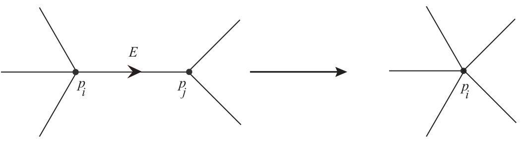 Figure 1
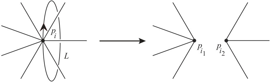 Figure 2
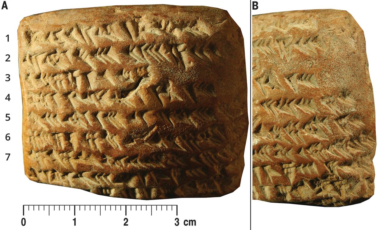 Figure 3
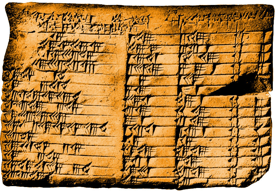 Figure 4
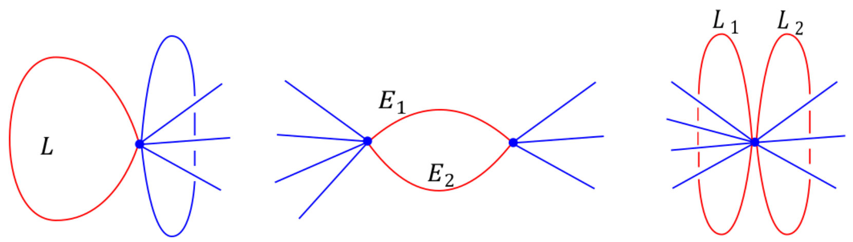 Figure 5
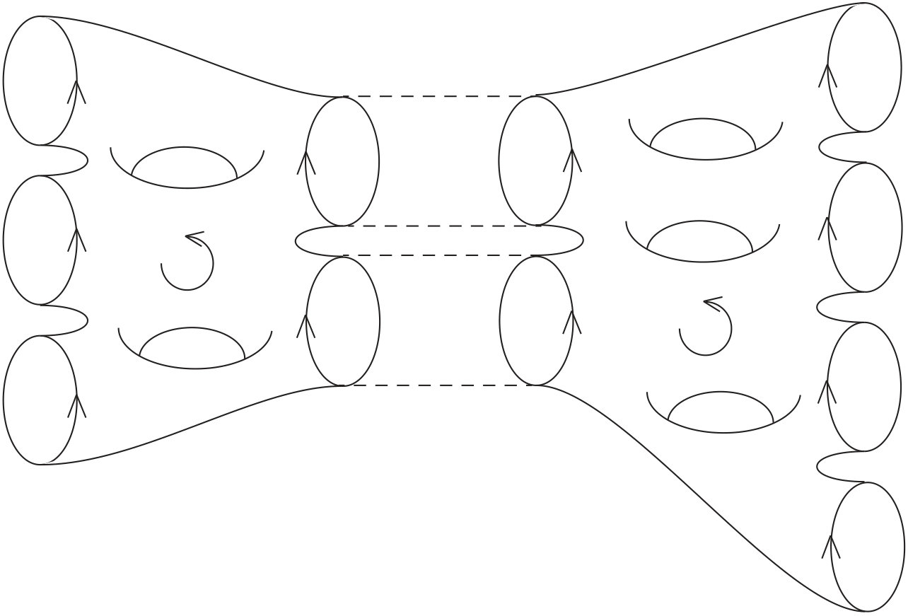 Figure 6
Peer Reviews
No public reviews on file for this paper yet. If you reviewed it on a platform where reviews are public (OpenReview, ICLR, NeurIPS, ICML), you can paste yours below so the community can read it here.
Videos
No videos yet. Explain this paper in a talk, walkthrough, or lecture? Add one.
An invitation to 2D TQFT and
quantization of Hitchin spectral curves
Olivia Dumitrescu
Olivia Dumitrescu: Department of Mathematics
Central Michigan University
Mount Pleasant, MI 48859, U.S.A.
and Simion Stoilow Institute of Mathematics
Romanian Academy
21 Calea Grivitei Street
010702 Bucharest, Romania
and
Motohico Mulase
Motohico Mulase: Department of Mathematics
University of California
Davis, CA 95616–8633, U.S.A.
and Kavli Institute for Physics and Mathematics of the Universe
The University of Tokyo
Kashiwa, Japan
Abstract.
This article consists of two parts. In Part 1, we present a formulation of two-dimensional topological quantum field theories in terms of a functor from a category of Ribbon graphs to the endofuntor category of a monoidal category. The key point is that the category of ribbon graphs produces all Frobenius objects. Necessary backgrounds from Frobenius algebras, topological quantum field theories, and cohomological field theories are reviewed. A result on Frobenius algebra twisted topological recursion is included at the end of Part 1.
In Part 2, we explain a geometric theory of quantum curves. The focus is placed on the process of quantization as a passage from families of Hitchin spectral curves to families of opers. To make the presentation simpler, we unfold the story using -opers and rank Higgs bundles defined on a compact Riemann surface of genus greater than . In this case, quantum curves, opers, and projective structures in all become the same notion. Background materials on projective coordinate systems, Higgs bundles, opers, and non-Abelian Hodge correspondence are explained.
Key words and phrases:
Topological quantum field theory; quantum curves; opers; Hitchin moduli spaces; Higgs bundles; Hitchin section; quantization; topological recursion.
2010 Mathematics Subject Classification:
Primary: 14H15, 14N35, 81T45; Secondary: 14F10, 14J26, 33C05, 33C10, 33C15, 34M60, 53D37
Contents
0. Preface: An inspiration from the past
A recent discovery of a cuneiform tablet dated around 350 to 50 B.C.E. suggests that ancient Babylonians must have used geometry of time-momentum space to establish accurate calculations of Jupiter’s orbit [87]. This impressive paper also contains the picture of the tablet which describes the Babylonian’s method of integration.
The orbit of the Jupiter is a graph in coordinate space-time. By considering the graph of momentum of the Jupiter in time-momentum space, Babylonians visualized integral of the momentum by the area underneath the curve, and using a trapezoidal approximation, they actually obtained an estimated value of the integral. This gives a prototype of Newton’s Fundamental Theorem of Calculus. This idea of Babylonians relating geometry of time-momentum space with the analysis of actual orbit of the Jupiter is striking, because it suggests their equal treatment of coordinate space the momentum space. Although it is a stretch, we could imagine the very foundation of symplectic geometry here.
Many mathematical cuneiform tablets recording numbers and algebraic calculations have been our source of imagination. The most famous is Plimpton 322 of around 1,800 B.C.E. (see Figure 0.2). It lists 15 Pythagorean numbers in the increasing order of hypotenuse angles from about 45 degrees to 60 degrees [88].
Babylonians seem to have known an algorithm to calculate an approximate value of the square root of any number. For example, there is a cuneiform tablet that shows the sexagesimal expansion of . Although there have been many speculations for practical purposes of Plimton 322 and mechanisms to come up with the listed numbers, our imagination goes to the surprise of the creator of the tablet. For the pair of numbers listed in the second and the third columns, is always a perfect square. Therefore, the square root algorithm terminates in a finite number of steps for these values, and gives an exact answer. They must have found a finiteness in the forest of infinity. This is a strong sentiment that resonates with our mind today.
The tablet of Figure 0.1 does not show any geometry. The author of [87] convincingly argues that behind the list of these seemingly meaningless numbers on the tablets, there is a profound geometric investigation of the planetary motion. Our imagination is piqued by the discovery: the interplay between algebra, geometry, and astronomy; and the equal treatment of momentum space and coordinate space. What the feeling of the authors of the tablet would have been, when they were creating it? It must have been a sharp happiness of discovery that mathematics correctly predicts the very nature surrounding us, such as planetary motion.
The accuracy of calculations of Babylonians is another astonishment, in addition to the lack of pictures. It is in sharp contrast to Euclid’s Elements, which was written around the same time in Greece. In Elements, we see many beautiful geometric pictures, and proofs. The discovery of axiomatic method culminated in it. This dichotomy, being able to calculate a quantity to a high precision, vs. having a proof of the formula based on a finiteness property, is our very motivation of writing these notes. There are a lot of amazing formulas around us in the direction that we describe. At this moment, we do not have the final understanding of them, yet.
In the first part of these lectures, we explore two-dimensional topological quantum field theories formulated in terms of cell graphs. A cell graph of type is the -skeleton of a cell-decomposition of a compact oriented topological surface of genus with labeled [math]-cells, or vertices. Such graphs are called in many different names: ribbon graphs, dessins d’enfants, maps, embedded graphs, etc. We use the terminology “cell graph” indicating the different nature of the graphs on surfaces, which record degeneration of surfaces. Although a cell graph is a -dimensional object, the notion of a face is well defined as a -cell of the cell decomposition that the cell graph defines on a given surface.
The degree of a vertex of a cell graph is the number of incident half-edges. We call a -cell an edge of the graph. As explained in our previous lecture notes [30], the number of cell graphs of type with the unique vertex of degree is , where
[TABLE]
is the -th Catalan number. A generating function
[TABLE]
of Catalan numbers satisfies an algebraic equation
[TABLE]
The story of [30, Section 2] tells us that enumeration problem of cell graphs of arbitrary type is solved by the quantization of the algebraic curve (0.0.1). The key formula for the quantization comes from the Laplace transform of a combinatorial equation [30, Catalan Recursion, Section 2.1]. There, the combinatorial formula is derived by analyzing the effect of edge-contraction operations on cell graphs.
The new story we wish to tell in these lectures is that the category of cell graphs carries the information of all two-dimensional topological quantum field theories. In Part 1 of this article, we will present an axiomatic setup of 2D TQFT. The key idea is simple: exact same edge-contraction operations characterize Frobenius algebras. When we contract an edge of a cell graph, two vertices collide. It represents multiplication. When we shrink a loop, since it is a cycle on the topological surface, the process breaks a vertex into two vertices. This is the operation of comultiplication. The topological structure of a cell graph makes these operations dual to one another in the context of Frobenius algebras.
We start with defining Frobenius algebras. Topological quantum field theories (TQFT) and cohomological field theories (CohFT) are introduced in the following sections. A category of cell graphs is defined. We explain that this category generates all Frobenius algebras. We then make a connection between cell graphs and 2D TQFT. The theory of topological recursion is a leitmotiv in this article. It is another manifestation of a quantization procedure. Since there are many review articles on topological recursion, we touch the subject only tangentially in this article. Our new result related to this topic is the 2D TQFT-twisted topological recursion, which is explained in the end of Part 1.
The cohomology ring of a closed oriented manifold is a Frobenius algebra. When we consider an even dimensional manifold and only even degree cohomologies
[TABLE]
then we have a commutative Frobenius algebra, which is equivalent to a 2D TQFT. The Gromov-Witten invariants of of genus [math] determine a quantum deformation of the ring , known as the big quantum cohomology. This quantum structure then defines a holomorphic object , the mirror of . Thus the holomorphic geometry of captures quantum cohomology of . Gromov-Witten invariants are generalized to arbitrary genera. Here arises a question:
Question 0.1**.**
What should be the holomorphic geometry on that corresponds to higher-genus Gromov-Witten theory of ?
If we consider the passage from genus [math] to higher genera Gromov-Witten theory as quantization, then on the side on , we need a quantized holomorphic geometry. A good candidate is the -module theory. The simplest such theory fitting to this context is the notion of quantum curves. The relation between quantum curves and B-model geometry is considered in [2, 19, 17, 27, 28, 30, 49, 50] and others. The key point for this idea to work is when the holomorphic geometry corresponding to the Gromov-Witten theory of is captured by an algebraic or analytic curve. These curves often appear in other areas of mathematics as spectral curves, such as integrable systems, random matrix theory, and Hitchin’s theory of Higgs bundles. A spectral curve naturally comes with a projection to a base curve, making it a covering of the base curve. A quantum curve is a -module on this base curve, quantizing the spectral curve.
Since a CohFT based on the Frobenius algebra plays a role similar to Gromov-Witten theory of , CohFT is a quantization of 2D TQFT. This process consists of two steps of quantizations. The first one is from the classical cohomology ring to its quantum deformation, which is the mirror geometry. If the mirror is a curve, then the second step should be parallel to the quantization of a spectral curve to a quantum curve. We may be able to understand the reconstruction [36] of CohFT based on a semi-simple Frobenius algebra from the 2D TQFT, that is obtained as the degree [math] part of the cohomology of the moduli space of stable curves, analogous to the construction of quantum curves.
Part 2 deals with quantum curves. Since the authors have produced a long article [30] explaining the relation between quantum curves and topological recursion, the present article is focused on geometry of the process of quantization of Hitchin spectral curves from a perspective of opers. Instead of providing a general theory of [25, 26, 31], we use to explain our ideas here. We will show that the classical notion of projective structures on a compact Riemann surface of genus studied by Gunning [51], -opers, and quantum curves of Hitchin spectral curves, are indeed the exact same notion. A conjecture of Gaiotto [42] relating non-Abelian Hodge correspondence and opers, together with its solution by [26], will be briefly explained in the final section.
Acknowledgement**.**
The authors are grateful to the organizers of the Warsaw Advanced School on Topological Quantum Field Theory for providing the opportunity to produce this article. They are in particular indebted to Piotr Sułkowski for constant encouragement and patience.
The joint research of authors presented in this article is carried out while they have been staying in the following institutions in the last four years: the American Institute of Mathematics in California, the Banff International Research Station, Institutul de Matematică “Simion Stoilow” al Academiei Roma͡ne, Institut Henri Poincaré, Institute for Mathematical Sciences at the National University of Singapore, Kobe University, Leibniz Universität Hannover, Lorentz Center Leiden, Mathematisches Forschungsinstitut Oberwolfach, Max-Planck-Institut für Mathematik-Bonn, and Osaka City University Advanced Mathematical Institute. Their generous financial support, hospitality, and stimulating research environments are greatly appreciated.
The research of O.D. has been supported by GRK 1463 Analysis, Geometry, and String Theory at the Leibniz Universität Hannover, Perimeter Institute for Theoretical Physics in Waterloo, and a grant from MPIM-Bonn. The research of M.M. has been supported by IHÉS, MPIM-Bonn, Simons Foundation, Hong Kong University of Science and Technology, Université Pierre et Marie Curie, and NSF grants DMS-1104734, DMS-1309298, DMS-1619760, DMS-1642515, and NSF-RNMS: Geometric Structures And Representation Varieties (GEAR Network, DMS-1107452, 1107263, 1107367).
Part I Topological Quantum Field Theory
1. Frobenius algebras
Throughout this article, we denote by a field of characteristic [math]. Most of the cases we consider or . Let be a finite-dimensional, unital, and associative algebra defined over a field . A bialgebra comes with an extra set of structures, including a comultiplication. Examples of bialgebras include the group algebra of a finite group . Its algebra structure is canonically determined by the multiplication rule of . However, the group algebra has two distinct co-algebra structures. One of which makes a Frobenius algebra, and the other makes it a Hopf algebra. This difference is reflected in which topological invariants we are dealing with. The Frobenius structure is useful for two-dimensional topology, and the Hopf structure is natural for three-dimensional topological invariants.
Let us start with defining Frobenius algebras.
Definition 1.1** (Frobenius algebras).**
A finite-dimensional, unital, and associative algebra over a field is a Frobenius algebra if there exists a linear map called counit such that for every , , or , for all implies that .
Proposition 1.2**.**
If and are Frobenius algebras, then and are also Frobenius algebras. Let us denote by the category of Frobenius algebras defined over . Then is a monoidal category.
Proof.
Denote by the counit of , . Then is a Frobenius algebra. Similarly,
[TABLE]
makes a Frobenius algebra. ∎
Example 1.3**.**
The one-dimensional vector space , with the identity map , is a simple commutative Frobenius algebra. More generally, by taking the direct sum and defining , we construct a semi-simple commutative Frobenius algebra .
Example 1.4**.**
The full matrix algebra consisting of matrices with is an example of a non-commutative simple Frobenius algebra for .
Example 1.5**.**
As mentioned above, the group algebra of a finite group is a Frobenius algebra. Here, we define by linearly extending the map whose value for every is given by
[TABLE]
Remark 1.6**.**
If we define for all , then the group algebra becomes a Hopf algebra.
Example 1.7**.**
The cohomology ring of an oriented compact differential manifold of with the cup product and
[TABLE]
is a Frobenius algebra.
The above example makes us wonder if an analogue of Poincaré pairing exists in a general Frobenius algebra. Indeed, the counterpart is a Frobenius bilinear form defined by
[TABLE]
in terms of the counit . The Frobenius form satisfies the Frobenius associativity
[TABLE]
The condition for the counit of Definition 1.1 exactly means that the Frobenius form is non-degenerate. It therefore defines a canonical isomorphism
[TABLE]
The isomorphism introduces a unique comultiplication by the following commutative diagram:
[TABLE]
Here, is the dual of the multiplication operation in . Since we are not assuming the multiplication to be commutative, we define the natural pairing
[TABLE]
by observing the order of entities as written. For example, for and , we calculate
[TABLE]
As the dual of the associative multiplication, the comultiplication is coassociative, i.e., it satisfies
[TABLE]
Note that the identity element corresponds to by , i.e., . This is because
[TABLE]
We now have the full set of data that defines a bialgebra. The algebra and coalgebra structures satisfy a compatibility condition, as described below.
Proposition 1.8**.**
The following diagram commutes:
[TABLE]
Remark 1.9**.**
Alternatively, we can define a Frobenius algebra as a bialgebra satisfying (1.0.7), together with a non-degenerate Frobenius form satisfying (1.0.2).
Proof.
Let be a -basis for , where . The bilinear form defines matrices
[TABLE]
It gives the canonical basis expansion of :
[TABLE]
From (1.0.4), we calculate
[TABLE]
using the pairing convention (1.0.5) and
[TABLE]
We then have
[TABLE]
Similarly,
[TABLE]
This completes the proof of Proposition 1.8. ∎
Remark 1.10**.**
We note that if is commutative, then the quantities
[TABLE]
are completely symmetric with respect to permutations of indices.
Definition 1.11** (Euler element).**
The Euler element of a Frobenius algebra is defined by
[TABLE]
In terms of basis, the Euler element is given by
[TABLE]
The Euler element provides the genus expansion of 2D TQFT, allowing us to calculate higher genus correlation functions from the genus [math] part of the theory.
Another application of (1.0.9) is the following formula that relates the multiplication and comultiplication:
[TABLE]
This is because
[TABLE]
2. TQFT
In this section, we briefly review TQFT. Although there have been explosive mathematical developments in higher dimensional topological quantum field theories mixing different dimensions during the last decade (see for example, [13, 67] and more recent work inspired by them), we restrict our attention to the two-dimensional speciality in these lectures. From now on, Frobenius algebras we consider are finite-dimensional, unital, associative, and commutative. It has been established (see [1, 16]) that 2D TQFT’s are classified by these types of Frobenius algebras.
The axiomatic formulation of conformal and topological quantum field theories was discovered in the 1980s by Atiyah [4] and Segal [89]. A -dimensional TQFT is a monoidal functor from the monoidal category of -dimensional closed (i.e., compact without boundary) oriented smooth manifolds with oriented -dimensional cobordism as morphisms, to the monoidal category of finite-dimensional vector spaces defined over a field . The monoidal structure in the category of -dimensional smooth manifolds is defined by the operation of taking disjoint union, which is a symmetric operation. Disjoint union with the empty set is the identity of this operation. Therefore, we define the monoidal category of -vector spaces by symmetric tensor products, with the field serving as the identity operation of tensor product. The functor satisfies the non-triviality condition
[TABLE]
and maps a disjoint union of smooth -dimensional manifolds to a symmetric tensor product of vector spaces.
Let us denote by an oriented closed smooth manifold of dimension , and by the same manifold with the opposite orientation. The functor satisfies the duality condition
[TABLE]
where is the dual vector space of . Suppose we have an oriented bordered -dimensional smooth manifold . The boundary is a smooth manifold of dimension , and the complement is an oriented smooth manifold of dimension . We give the orientation induced from to its boundary . The TQFT functor then gives an element
[TABLE]
If is closed, i.e., , then
[TABLE]
is a number that represents a topological invariant of .
Now consider a bordered oriented smooth manifold with boundary
[TABLE]
meaning that the two separate boundaries carry different orientations. We choose that is given the induced orientation from , and the opposite orientation. We interpret the situation as giving an oriented cobordism from to . In this case, the functor defines an element , or equivalently, a linear map
[TABLE]
Suppose we have another smooth manifold with boundary
[TABLE]
corresponding to a linear map
[TABLE]
We can then smoothly glue and along the common boundary component forming a new manifold
[TABLE]
Clearly
[TABLE]
and gives a cobordism from to . The Atiyah-Segal sewing axiom [4] asserts that
[TABLE]
A -dimensional TQFT defines a topological invariant for each closed -manifold . The essence of TQFT is to break into simpler pieces by cutting along -dimensional submanifolds, and represent the invariant from that of simpler pieces. The situation is special for the case of 2D TQFT. First of all, we already know all topological invariants of a closed surface. They are just functions of the genus of the surface. So there should be no reason for another theory to study them. Since there is only one -dimensional connected compact smooth manifold, a 2D TQFT is based on a single vector space
[TABLE]
and its tensor products. What else could we gain?
The biggest surprise is that a 2D TQFT is further quantized [15, 24, 48, 63]. This process starts with a Frobenius algebra of (0.0.2). It is quantized to a quantum cohomology, and then further to Gromov-Witten invariants. Construction of spectral curves, and then quantizing them, have a parallelism to this story. This is the story we now explore in this and the next sections, but only to take a snapshot of the converse direction, i.e., from a quantum theory to a classical theory.
Let us denote by a connected, bordered, oriented, smooth surface of genus with boundary circles. This is a surface obtained by removing disjoint open discs from a compact oriented two-dimensional smooth manifold of genus without boundary. We assume that the boundary of itself is a smooth manifold, hence it is a disjoint union of circles. We give the induced orientation from the surface to boundary circles, and the opposite orientation to the boundary circles. The surface gives a cobordism of circles to circles. The orientation-preserving diffeomorphism class of such a surface is determined by the genus and the two number and of boundary circles with different orientations. Therefore, the oriented equivalence class of cobordism is also determined by . The TQFT functor then assigns to each cobordism a multilinear map
[TABLE]
which is completely determined by the label . This is the special situation of the two-dimensionality of TQFT, reflecting the simple topological classification of surfaces.
Suppose we have another cobordism of genus from circles to circles, with orientation on the circles induced from the surface, and the opposite orientation on circles. We can compose two cobordisms, sewing the circles of the first cobordism with the circles of the second. Here, we notice that on each pair of circles, one from the first surface and the other from the second, the orientations are the same, and hence we can put one on top of the other. Therefore, the orientations of the two surfaces are consistent after sewing. This sewing process generates a new surface of genus . This is because the pairs of circles sewed together create handles (see Figure 2.1). The sewing axiom of Atiyah-Segal [4] then requires that the functor associates the composition of linear maps to the composition of cobordisms. In our situation, the composition of two maps generates a new map
[TABLE]
corresponding to the sewing of cobordisms.
The sewing procedure can be generalized, allowing partial sewing of the boundary circles of matching orientation. For example, if and , then gluing only pairs of circles, we have a composition
[TABLE]
Furthermore, since TQFT does not require cobordism to be given by a connected manifold, we can stack up disjoint union of surfaces and apply partial sewing to create a variety of linear maps from to .
It was Dijkgraaf [16] who noticed the equivalence between 2D TQFTs and commutative Frobenius algebras. We can see the resemblance immediately. On the vector space , we have operations defined by
[TABLE]
A connected cobordism of incoming circles and outgoing circles is classified by the genus of the surface. It does not depend on the history of how the cobordisms are glued together. Thus the diffeomorphism classes of surfaces after sewing cobordisms tell us relations among the operations of (LABEL:operations). For example,
[TABLE]
which is (1.0.1). Associativity of multiplication comes from uniqueness of the topology of with one boundary circle carrying the induced orientation and three the opposite orientation. Changing the orientation of each boundary component to its opposite provides coassociativity. In this way acquires a bialgebra structure. To assure duality between algebra and coalgebra structures, we need to impose another condition here: non-degeneracy of . Then becomes a commutative Frobenius algebra.
Conversely, if we start with a finite-dimenionsal commutative Frobenius algebra , then we first construct on the list of (LABEL:operations). More general maps are constructed by partial sewing (2.0.3). By construction, all these maps are associated with cobordism of circles, and hence determine a 2D TQFT [1].
With the above considerations, we give the following definition.
Definition 2.1** **(Two-dimensional
Topological Quantum Field Theory).
Let be a set of data consisting of a finite-dimensional vector space over , a non-trivial linear map , and an isomorphism . A Two-dimensional Topological Quantum Field Theory is a system consisting of linear maps
[TABLE]
satisfying the following axioms.
- •
TQFT 1. Symmetry:
[TABLE]
is symmetric with respect to the -action on the domain.
- •
TQFT 2. Non-triviality:
[TABLE]
- •
TQFT 3. Duality:
[TABLE]
- •
TQFT 4. Sewing:
[TABLE]
Remark 2.2**.**
As noted above, the vector space acquires the structure of a commutative Frobenius algebra from these axioms. Conversely, if is a commutative Frobenius algebra, then of (LABEL:operations) can be extended to that satisfy the TQFT axioms.
3. Cohomological field theory
Recall that for any oriented closed manifold , its cohomology ring is a Frobenius algebra defined over . If we restrict ourselves to even dimensional manifold and consider only even part of the cohomology, then is a finite-dimensional commutative Frobenius algebra. This Frobenius algebra naturally defines a 2D TQFT. The role of a TQFT in general dimension is to represent a topological invariant of higher dimensional manifolds. We are now seeing that the classical topology of a manifold is a 2D TQFT. Changing our point of view, we can ask if we start with , then how do we find the corresponding 2D TQFT? Of course the Frobenius algebra structure automatically determine the unique 2D TQFT as we have seen in Section 2. But then the picture of sewing cobordisms is lost in this algebraic formulation. What is the role of the cobordism of circles in the context of understanding the manifold ?
The amazing vision emerged in the early 1990s is that 2D TQFT can be further quantized into Gromov-Witten theory, which produces quantum topological invariants of that cannot be reduced to classical invariants. This epoch making discovery was one of the decisive moments of the fruitful interaction of string theory and geometry, which is still continuing today.
String theory deals with flying strings in a space-time manifold . The trajectory of a moving string is a curved cylinder embedded in the manifold , like a duct pipe in the attic. When strings are considered as quantum objects, they can interact one another. For example, Figure 2.1 can be interpreted as a string of string interactions. First, three strings collide in a complicated interaction to produce two strings. The complexity of the interaction is classified as “” in terms of the genus of the first surface. These two strings created in the first interaction then collide in an even more complicated (i.e., ) interaction to produce four strings in the end. The trajectory of these interactions then forms a bordered surface of genus with boundary components embedded in the space-time .
Models for string theory were originally introduced to understand how the space-time dictates string interactions. In this process, the importance of Calabi-Yau spaces was recognized, through considerations on the consistency of string theory as a physical theory. By changing the point of view , researchers then noticed that a simple model of string interactions could be used to obtain a totally new class of topological invariants of itself. These new invariants are not necessarily captured by the classical topology, such as (co)homology groups and homotopy groups. We use the terminology of quantum topological invariants for the invariants obtained by string theory considerations.
Gromov-Witten theory is a mathematically rigorous interpretation of a model for a quantum string theory. A trajectory of interacting strings in is the image of a map
[TABLE]
from a bordered surface into . Recall that the fundamental group of is determined by the connectivity of the pointed loop space
[TABLE]
which is the moduli space of differentiable maps from to that send a reference point to . In the same spirit, Gromov-Witten invariants are defined by looking at the classical topological invariants of appropriate moduli spaces of maps from to . When we have the notion of size of a string, the trajectory has a metric on it. If the ambient manifold has a geometric structure, such as a symplectic structure, complex structure, or a Kähler structure, then the map needs to be compatible with the structures of the source and the target. For example, if is Kähler, then we give a complex structure on that is compatible with the metric it has, and require that is a holomorphic map. Technical difficulties arise in defining moduli spaces of such maps. Even the moduli spaces are defined, they are often very different objects from the usual differentiable manifolds. We need to extend the notion of manifolds here. Thus identifying reasonable classical topological invariants of these spaces also poses a difficult problem.
The simplest scenario is the following: We take to be just a single point. Of course nobody wants to know the topological structure of a point. We all know it! By exploring the Gromov-Witten theory of a point, we learn the structure of the theory itself. Since we can map anything to a point, a point may not be such a simple object, after all. It is like considering a vacuum in physics. Again, anything can be thrown into a vacuum. A quantum theory of a vacuum is inevitably a rich theory.
When is a point, we consider all incoming and outgoing strings to be infinitesimally small. Thus the surfaces we are considering become closed, and boundary components are just several points identified on them. A metric on a closed surface naturally gives rise to a unique complex structure, making it a compact Riemann surface. And every compact Riemann surface acquires a unique projective algebraic structure, making it a projective algebraic curve. Since we are allowing strings to become infinitesimally small during the interaction, the trajectory may contain a process of an embedded in the surface shrinking to a point, and then becoming a finite size circle again a moment later. Such a process can be understood in complex algebraic geometry as a nodal singularity of an algebraic curve. Locally, every nodal singularity of a curve is the same as the neighborhood of the origin of a singular algebraic curve
[TABLE]
We are talking about an abstract notion of trajectories here, because nothing can move in . In terms of the map idea (3.0.1), we note that there is a unique map from any projective algebraic curve to a point, which satisfies any reasonable requirement of maps such as being a morphism of algebraic varieties. Then the moduli space of all maps simply means the moduli space of the source.
A stable curve is a projective algebraic curve with only nodal singularities and a finite number of smooth points marked on the curve such that it has only a finite number of algebraic automorphisms fixing each marked point. We recall that the holomorphic automorphism group of ,
[TABLE]
acts on triply transitively. The number of automorphisms fixing up to points is always infinity. Since is compact and three-dimensional, if we choose three distinct points on and require the automorphism to fix each of these points, then we have only finitely many choices. Actually in our case, it is unique. For an elliptic curve , since it is an abelian group, acts on transitively. To avoid these translations, we need to choose a point on . We can naturally identify it as the identity element of the elliptic curve as a group. Automorphisms of an elliptic curve fixing a point then form a finite group. If a compact Riemann surface has genus , then it is known that the order of the analytic automorphism group is bounded by
[TABLE]
This bound comes from hyperbolic geometry. It is easy to see the finiteness. First, we note that universal covering of is the upper half plane
[TABLE]
and is constructed by the quotient
[TABLE]
through a faithful representation
[TABLE]
of the fundamental group of into the automorphism group of . Every holomorphic automorphism of extends to an automorphism of . We know that does not have any non-trivial holomorphic vector field . If it did, then would be a differentiable vector field with isolated zeros, and each zero comes with positive index, because locally it is given by . We learn from topology that the sum of the indices of isolated zeros of a vector field on is equal to . It is a contradiction. Thus is a discrete subgroup. Since is compact, is finite.
An algebraic curve is stable if and only if (1) every singularity is nodal, and (2) every irreducible component of has a finite number of automorphisms. The second condition means that the total number of smooth marked points and singular points of that are on has to be or more if , and or more if . There is no condition for an irreducible component of genus two or more.
For a pair of integers and in the stable range , we denote by the moduli space of stable curves of genus and smooth marked points. It is a complex orbifold of dimension . Quantum topological invariants of a point is then realized as classical topological invariants of . Alas to this day, we cannot identify the cohomology groups for all values of . From the very definition of these moduli spaces, we can construct many concrete cohomology classes on each of , called tautological classes. What we do not know is indeed how much more we need to know to determine all of . The surprise of Witten’s conjecture [93], proved in [62], is that we can actually explicitly write intersection relations of certain tautological classes for all values of and .
Among many different proofs available for the Witten conjecture (see for example, [61, 62, 71, 72, 80, 85]), [72, 80] deal with recursive relations among surfaces much in the same spirit of TQFT. These relations are first noticed in [20]. We will discuss these relations in connection to topological recursion later in these lectures.
Geometric relations among ’s for different values of have a simple meaning. Let us denote by the moduli space of smooth -pointed curves. Then the boundary
[TABLE]
consists of points representing singular curves. Simplest singular stable curve has one nodal singularity, which can be described as collision of two smooth points. Analyzing how these singularities occur via degeneration, we come up with three types of natural morphisms among the moduli spaces . They are the forgetful morphisms
[TABLE]
which simply erase one of the marked points on a stable curve, and gluing morphisms
[TABLE]
that construct boundary strata of . Under a gluing morphism, we put two smooth points of stable curves together to form a one nodal singularity. The first one glues two points on the same curve together, and one each on two curves.
The fiber of at a stable curve is the curve itself, because another marked point can be placed anywhere on . Thus is a universal family of curves parameterized by the base moduli space . When we place the extra marked point at , , then as the point of on the fiber of , the data represented is a singular curve obtained by joining itself with a at the location of , but the two marked points are actually placed on the line . Assigning this singular curve to defines a section
[TABLE]
which is a right inverse of . Geometrically, sends to the point on the fiber . Obviously,
[TABLE]
is the identity map.
Gromov-Witten theory for a Kähler manifold [15] concerns topological structure of the moduli space
[TABLE]
of stable holomorphic maps from a nodal curve with smooth marked points to such that the homology class of the image agrees with a prescribed homology class . Here, stability of a map is again defined by imposing the finiteness of possible automorphisms. Giving a definition of this moduli space is beyond our scope of this article. We refer to [15]. The moduli space, if defined, should come with natural maps
[TABLE]
where the forgetful map assigns the stabilization of the source to the map by forgetting about the map itself, and
[TABLE]
is the value of at the -th marked point . Stabilization means that evey irreducible component of that is not stable is shrunk to a point. If we indeed know the moduli space and that its cohomology theory behaves as we expect, then we would have
[TABLE]
where is the Gysin map defined by integration along fiber. If were a manifold, and the map were a fiber bundle, then would have been locally a direct product, hence the Gysin map associated with would be defined by integrating de Rham cohomology classes of along fiber of . Choose any cohomology classes of . We then could have defined the Gromov-Witten invariants by
[TABLE]
In general, however, construction of the Gysin map does not work as we hope. This is due to the complicated nature of the moduli space , which often has components of unexpected dimensions. The remedy is to define the virtual fundamental class of the expected dimension, and avoid the use of by defining
[TABLE]
See [15] for more detail.
Now recall that is a Frobenius algebra. Although Gromov-Witten theory goes through a big black box , what we wish is a map
[TABLE]
whose integral over gives the quantum invariants of . Then what are the properties that Gromov-Witten invariants should satisfy? Can we list the properties as axioms for the above map so that we can characterize Gromov-Witten invariants? This was one of the motivations of Kontsevich and Manin to introduce CohFT in [63].
As we see below, a 2D TQFT can be obtained as a special case of a CohFT. The amazing relation between TQFT and CohFT, i.e., the reconstruction of CohFT from its restriction to TQFT due to Givental and Teleman [48, 91], plays a key role in many new developments (see for example, [3, 36, 39, 68]), some of which are deeply related with topological recursion.
Definition 3.1** **(Cohomological Field Theory
[63]).
Let be a finite-dimensional, unital, associative, and commutative Frobenius algebra with a basis . A Cohomological Field Theory is a system consisting of linear maps
[TABLE]
defined for in the stable range and satisfying the following axioms:
[TABLE]
where is a disjoint partition of the index set, and the tensor product operation on the right-hand side is performed via the Künneth formula of cohomology rings
[TABLE]
Remark 3.2**.**
The condition says that the product of the Frobenius algebra is determined by the -value of the Gromov-Witten invariants.
Proposition 3.3** (2D TQFT is a CohFT).**
Every 2D TQFT is a CohFT that takes values in . More precisely, let be a 2D TQFT. Then satisfies the CohFT axioms, by identifying .
Proof.
Since is connected, the three types of morphisms (3.0.3), (3.0.4), and (3.0.5) all produce isomorphisms of degree [math] cohomologies. Thus the axioms CohFT 1–3 become
[TABLE]
We wish to show that (3.0.8)-(3.0.10) are consequences of the partial sewing axiom (2.0.8) of TQFT under the identification .
Since , we have
[TABLE]
from (2.0.8), which is (3.0.8). Here, is the composition taken at the -th slot of the input variables of . Next, we need to identify . Since , we see that . Denoting by to indicate composition taking at the last two slots of variables, we have (3.0.9)
[TABLE]
If we have two disjoint sets of variables and , then we can apply composition of simultaneously to two different maps. For example, we have
[TABLE]
which is (3.0.10).
Notice that a linear map
[TABLE]
is equivalent to . Thus we can re-construct a map from by
[TABLE]
where is the isomorphism of (1.0.3). For the case of , , and , (3.0.11) implies that
[TABLE]
for . Or equivalently, we have
[TABLE]
This completes the proof. ∎
Conversely, the degree [math] part of the cohomology of a CohFT is a 2D TQFT.
Proposition 3.4** **(Restriction of CohFT to the degree [math]
part of the cohomology ring).
Let be a CohFT associated with a Frobenius algebra . The Frobenius algebra itself defines a unique 2D TQFT . Denote by
[TABLE]
the restriction of the cohomology ring to its degree [math] component, and define
[TABLE]
Then we have the equality of maps
[TABLE]
for all with . In other words, the degree [math] restriction of a CohFT is the 2D TQFT determined by the Frobenius algebra .
Proof.
We already know that defines a CohFT with values in . We need to show that this CohFT is exactly the degree [math] restriction of the given CohFT we start with.
First we extend to the unstable range by
[TABLE]
We then note that from (LABEL:operations) and (3.0.15), we see that (3.0.14) holds for and . The general case of (3.0.14) follows by induction on , provided that is appropriately defined. This is because (3.0.9) and (3.0.10) are induction formula recursively generating from those with smaller values of and . Since
- •
Case of (3.0.9): ,
- •
Case of (3.0.10):
we see that the complexity is always reduced by in each of the recursive formulas.
Finally, we see that since is just a point as we have noted above in the discussion of , we have . Hence
[TABLE]
which makes (3.0.14) holds for all values of . This completes the proof. ∎
Remark 3.5**.**
The above two propositions show that a 2D TQFT can be defined either just by a commutative Frobenius algebra , by a system of maps satisfying the TQFT axioms, or the degree [math] part of a CohFT. From now on, we use to denote a 2D TQFT, which is less cumbersome and easier to deal with.
Proposition 3.6**.**
The genus [math] values of a 2D TQFT is given by
[TABLE]
Proof.
This is a direct consequence of CohFT 3 and (1.0.9). ∎
One of the original motivations of TQFT [4, 89] is to identify the topological invariant of a closed manifold . In our current setting, it is defined as
[TABLE]
for a closed oriented surface of genus . Here, is an element of , and is the canonical isomorphism (1.0.3).
Proposition 3.7**.**
The topological invariant of (3.0.18) is given by
[TABLE]
where is the Euler element of (1.0.12).
Lemma 3.8**.**
We have
[TABLE]
Proof.
This follows from
[TABLE]
for every . ∎
Proof of
Proposition 3.7.
Since the starting case follows from the above Lemma, we prove the formula by induction, which goes as follows:
[TABLE]
∎
A closed genus surface is obtained by sewing genus pieces with one output boundaries to a genus [math] surface with input boundaries. Since the Euler element is the output of the genus surface with one boundary, we obtain the same result
[TABLE]
Finally we have the following:
Theorem 3.9**.**
The value of a 2D TQFT is given by
[TABLE]
Proof.
The argument is the same as the proof of Proposition 3.7:
[TABLE]
∎
4. Category of cell graphs
In the original formulation of 2D TQFT, the operations of multiplication and comultiplication are associated with an oriented surface of genus [math] with three boundary circles. In this section, we introduce a category of ribbon graphs, which carries the information of all finite-dimensional Frobenius algebras. To avoid unnecessary confusion, we use the terminology of cell graphs in this article, instead of more common ribbon graphs. Ribbon graphs naturally appear for encoding complex structures of a topological surface (see for example, [62, 75]). Our purpose of using ribbon graphs are for degeneration of stable curves, and we label vertices, instead of faces, of a ribbon graph.
Definition 4.1** (Cell graphs).**
A connected cell graph of topological type is the -skeleton of a cell-decomposition of a connected closed oriented surface of genus with labeled [math]-cells. We call a [math]-cell a vertex, a -cell an edge, and a -cell a face, of the cell graph. We denote by the set of connected cell graphs of type . Each edge consists of two half-edges connected at the midpoint of the edge.
Remark 4.2**.**
- •
The dual of a cell graph is a ribbon graph, or Grothendieck’s dessin d’enfant. We note that we label vertices of a cell graph, which corresponds to face labeling of a ribbon graph. Ribbon graphs are also called by different names, such as embedded graphs and maps.
- •
We identify two cell graphs if there is a homeomorphism of the surfaces that brings one cell-decomposition to the other, keeping the labeling of [math]-cells. The only possible automorphisms of a cell graph come from cyclic rotations of half-edges at each vertex.
Definition 4.3** (Directed cell graph).**
A directed cell graph is a cell graph for which an arrow is assigned to each edge. An arrow is the same as an ordering of the two half-edges forming an edge. The set of directed cell graphs of type is denoted by .
Remark 4.4**.**
A directed cell graph is a quiver. Since our graph is drawn on an oriented surface, a directed cell graph carries more information than its underlying quiver structure. The tail vertex of an arrowed edge is called the source, and the head of the arrow the target, in the quiver language.
To label vertices, we normally use the -set
[TABLE]
However, it is often easier to use any totally ordered set of elements for labeling. The main reason we label the vertices of a cell graph is we wish to assign an element of a -vector space to each vertex. In this article, we consider the case that a cell graph defines a linear map
[TABLE]
The set of values of these functions can be more general. We discuss some of the general cases in [33].
An effective tool in graph enumeration is edge-contraction operations. Often edge contraction leads to an inductive formula for counting problems of graphs. The same edge-contraction operations acquire algebraic meaning in our consideration.
Definition 4.5** (Edge-contraction operations).**
There are two types of edge-contraction operations applied to cell graphs.
- •
ECO 1: Suppose there is a directed edge in a cell graph , connecting the tail vertex and the head vertex . We contract in , and put the two vertices and together. We use for the label of this new vertex, and call it again . Then we have a new cell graph with one less vertices. In this process, the topology of the surface on which is drawn does not change. Thus genus of the graph stays the same.
- •
We use the notation for the edge-contraction operation
[TABLE]
- •
ECO 2: Suppose there is a directed loop in at the -th vertex . Since a loop in the -skeleton of a cell decomposition is a topological cycle on the surface, its contraction inevitably changes the topology of the surface. First we look at the half-edges incident to vertex . Locally around on the surface, the directed loop separates the neighborhood of into two pieces. Accordingly, we put the incident half-edges into two groups. We then break the vertex into two vertices, and , so that one group of half-edges are incident to , and the other group to . The order of two vertices is determined by placing the loop upward near at vertex . Then we name the new vertex on its left by , and on its right by .
Let denote the possibly disconnected graph obtained by contracting and separating the vertex to two distinct vertices labeled by and .
- •
If is connected, then it is in . The loop is a loop of handle. We use the same notation to indicate the edge-contraction operation
[TABLE]
- •
If is disconnected, then write , where
[TABLE]
The edge-contraction operation is again denoted by
[TABLE]
In this case we call a separating loop. Here, vertices labeled by belong to the connected component of genus , and those labeled by are on the other component of genus . Let (reps. ) be the reordering of (resp. ) in the increasing order. Although we give labeling to the two vertices created by breaking , since they belong to distinct graphs, we can simply use for the label of and the same for . The arrow of translates into the information of ordering among the two vertices and .
Remark 4.6**.**
Let us define for a graph . Then every edge-contraction operation reduces exactly by . Indeed, for ECO 1, we have
[TABLE]
The ECO 2 applied to a loop of handle produces
[TABLE]
For a separating loop, we have
[TABLE]
The motivation for our introduction of directed cell graphs is that we need them when we deal with non-commutative Frobenius algebras. The operation of taking disjoint union is symmetric. Therefore, 2D TQFT inevitably leads to a commutative Frobenius algebra. The advantage of our formalism using directed cell graphs is that we can deal with non-commutative Frobenius algebras and non-symmetric tensor products.
For the purpose of presenting the idea of the category of cell graphs as simple as possible, we restrict ourselves to undirected cell graphs in this article. Therefore, we will only recover commutative Frobenius algebras and usual 2D TQFT. A more general theory will be given in [33].
We now introduce the category of cell graphs. The most unusual point we present here is that a morphism between cell graphs is not a cell map. Recall that a cell map from a cell graph to another cell graph is a topological map between -dimensional cell complexes. Thus sends a vertex of to a vertex of , and an edge of to either an edge or a vertex of , keeping the incidence relations. In particular, a cell map is continuous with respect to the topological structure on cell graphs indued from the surface on which they are drawn.
Definition 4.7** (Category of cell graphs).**
The category of cell graphs is defined as follows.
- •
The set of objects of is the set of all cell graphs:
[TABLE]
- •
A morphism
[TABLE]
is a composition of a finite sequence of edge-contraction operations and cell graph automorphisms. In particular, . If there is no way to bring to by consecutive applications of edge-contraction operations and automorphisms, then we define , even though there may be cell maps between them.
Remark 4.8**.**
The triple forms a symmetric monoidal category.
Remark 4.9**.**
Automorphisms of a cell graph and ECOs of the first kind are cell maps, but ECO 2 operations are not. When an ECO 2 is involved, a morphism between cell graphs does not have to be a cell map. Even it may not be a continuous map.
Example 4.10**.**
A few simple examples of morphisms are given below. Note that vertices are all labeled, and automorphisms are required to keep labeling.
[TABLE]
In (4.0.10), we note that is equal to , because they both produce the same result . The cell graph of the left of (4.0.11) and (4.0.12) has an automorphism that interchanges and . Thus as an edge-contraction operation, . Note that there is a covering cell map for the case of (4.0.11) that sends both edges and on to the single loop of , and the two vertices on the first graph to the single vertex on the second. Since it is not an edge-contraction, this cell map is not a morphism. The morphism of (4.0.12) is not a cell map, since it is not continuous.
Let be the category of finite-dimensional -vector spaces. The triple
[TABLE]
forms a monoidal category. Again for simplicity, we are concerned only with symmetric tensor products in this article, so we consider a symmetric monoidal category. A -object in is a pair consisting of a vector space and a linear map . We denote by the category of -objects in . It has the unique final object . Therefore,
[TABLE]
is again a monoidal category. We denote by
[TABLE]
the endofunctor category of the monoidal category , which consists of monoidal functors as its objects, and their natural transformations as morphisms. Schematically, we have
[TABLE]
Here, the triangle on the left shows two objects and of , and a morphism between them. The prism shape on the right represents two monoidal endofunctors and that assigns
[TABLE]
and a natural transformation among them. The final object of is the functor
[TABLE]
which assigns the final object of the codomain to everything in the domain . With respect to the tensor product and the above functor (4.0.14) as its identity object, the endofunctor category is again a monoidal category.
Definition 4.11** (ECO functor, [33]).**
The ECO functor is a monoidal functor
[TABLE]
satisfying the following conditions.
- •
The graph consisting of only one vertex and no edge corresponds to the identity functor
[TABLE]
- •
Each graph corresponds to a functor
[TABLE]
- •
Edge-contraction operations correspond to natural transformations.
Let us recall the notion of Frobenius object.
Definition 4.12** (Frobenius object).**
Let be a symmetric monoidal category. A Frobenius object is an object together with morphisms
[TABLE]
satisfying the following conditions:
- •
is a monoid object in .
- •
is a comonoid object in .
We also require the compatibility condition (1.0.7) among morphisms and :
[TABLE]
Since we are considering the monoidal category of -objects in , there is a priori no notion of in . The existence of the morphism requires a non-degeneracy condition. The following theorem is proved in [33].
Theorem 4.13** (Generation of Frobenius objects [33]).**
An object of is a Frobenius object if defines a non-degenerate symmetric bilinear form on .
5. 2D TQFT from cell graphs
The result of Section 3 tells us that a 2D TQFT can be defined as a system of linear maps
[TABLE]
defined for all values of and , satisfying a set of conditions. The required conditions are the following: First, is a CohFT for . In addition, we require that
[TABLE]
In this section we give a different formulation of a 2D TQFT, based on cell graphs and a different set of axioms. Our ultimate goal is to relate 2D TQFT, CohFT, mirror symmetry, topological recursion, and quantum curves. Later in these lectures, we introduce quantum curves. Relations between all these subjects will be discussed elsewhere [33].
Theorem 5.1** (Graph independence [29]).**
Let be a Frobenius object under the ECO functor of Definition 4.11. Then every connected cell graph gives rise to the same map
[TABLE]
where is the Euler element of (1.0.12).
Corollary 5.2** (ECO implies TQFT).**
Define for every . Then is a 2D TQFT.
Proof.
Since the value of (5.0.3) is the same as (3.0.21), it is a 2D TQFT. ∎
The rest of the section is devoted to proving Theorem 5.1. We first give three examples of graph independence.
Lemma 5.3** (Edge-removal lemma).**
Let .
- •
Case 1.* There is a disc-bounding loop in . Let be the graph obtained by simply removing from . Note that we are not contracting .*
- •
Case 2.* The graph containts two edges and between two distinct vertices and that bound a disc. Let be the graph obtained by removing . Here again, we are just eliminating .*
- •
Case 3.* Two loops, and , in are attached to the -th vertex . If they are homotopic, then let be the graph obtained by removing from .*
In each of the above cases, we have
[TABLE]
Proof.
Case 1. Contracting a disc-bounding loop attached to creates , where consists of only one vertex and no edges. The natural transformation corresponding to ECO 1 then gives
[TABLE]
Case 2. Contracting Edge makes a disc-bounding loop at . We can remove it by Case 1. Note that the new vertex is assigned with . Restoring makes the graph exactly the one obtained by removing from . Thus (5.0.4) holds.
Case 3. Contracting Loop makes a disc-bounding loop. Hence we can remove it by Case 1. Then restoring creates a graph obtained from by removing . Thus (5.0.4) holds. ∎
Remark 5.4**.**
The three cases treated above correspond to removing degree and vertices from the dual ribbon graph.
Definition 5.5** (Reduced graph).**
A cell graph is reduced if it does not contain any disc-bounding loops or disc-bounding bigons. In terms of dual ribbon graphs, the dual of a reduced cell graph has no vertices of degree or .
We can see from Lemma 5.3, Case 1, that every graph gives the same map
[TABLE]
Similarly, Cases 2 and 3 of Lemma 5.3 show that every graph defines
[TABLE]
This is because we can remove all edges and loops but one that connects the two vertices. Then by the natural transformation corresponding to ECO 1, the value of the assignment is .
Proof of Theorem 5.1.
We use the induction on . The base case is , or , for which the theorem holds by (5.0.5). Assume that (5.0.3) holds for all with . Now let be a cell graph of type such that . Choose an arbitrary straight edge of that connects two distinct vertices, say and . Then the natural transformation of contracting this edge to gives
[TABLE]
If we have chosen an arbitrary loop attached to , then its contraction by ECO 2 gives two cases, depending on whether the loop is a loop of handle or a separating loop. For the former case, we have a graph , and by appealing to (1.0.9) and (1.0.13), we obtain
[TABLE]
For the case of a separating loop, ECO 2 makes , and we have
[TABLE]
Therefore, no matter how we apply ECO 1 or ECO 2, we always obtain the same result. This completes the proof. ∎
6. TQFT-valued topological recursion
There is a direct relation between a Frobenius algebra and Gromov-Witten theory when is given by the big quantum cohomology of a target space. Since these Frobenius algebras are usually infinite-dimensional over the ground field, they do not correspond to a 2D TQFT discussed in the previous sections. But for the case that the target space is [math]-dimensional, the TQFT indeed captures the whole Gromov-Witten theory.
In this section, we present a general framework. Fundamental examples are , which gives -class intersection numbers on , and the center of the group algebra of a finite group , which produces Gromov-Witten invariants of the classifying space . The first example is considered in [29, 30]. The latter case will be discussed elswhere [33].
We wish to solve a graph enumeration problem, where as a graph we consider a cell graph, and each of its vertex is colored by a parameter . We also impose functoriality under the edge-contraction of Definition 4.5 for this coloring. The ECOs reduce the complexity of coloring considerably, because the functoriality makes the coloring process graph independent, as we have shown in the last section. Thus the answer is just the number of graphs times the value for each topological type . Here comes the difficulty: there are infinitely many graphs for each topological type, since we allow multiple edges and loops. The standard idea for such counting problem is to appeal to the Laplace transform, which is introduced by Laplace for this particular context of counting an infinite number of objects. Let us denote by
[TABLE]
the set of all cell graphs with labeled vertices of degrees . Denoting by the number of -cells in a cell-decomposition of a surface of genus , , we have , and Therefore, (6.0.1) is a finite set.
Counting processes become easier if we do not have any object with non-trivial automorphism. There are many ways to eliminate automorphism, for example, the minimalistic way of imposing the least possible conditions, or an excessive way to kill automorphisms but for the most objects the conditions are redundant. Actually, it is known that most of the cell graphs counted in (6.0.1) are without any non-trivial automorphisms. Since any possible automorphism induces a cyclic permutation of half-edges incident to each vertex, the easiest way to disallow any automorphism is to assign an outgoing arrow to one of these half-edges, as in [34, 79] (but not as a quiver). An automorphism should preserve the arrowed half-edges, in addition to labeled vertices. We denote by
[TABLE]
the set of arrowed cell graphs with labeled vertices of degrees , and by
[TABLE]
its cardinality. This number is always a non-negative integer, and is the -th Catalan number.
We use the notation of Corollary 5.2 for . We are interested in considering the -weighted TQFT
[TABLE]
and applying the edge-contraction operations to these maps. We contract the edge of that carries the outgoing arrow at the first vertex , then place a new arrow to the half-edge next to the original half-edge with respect to the cyclic ordering induced by the orientation of the surface. If the edge that carries the outgoing arrow at is a loop, then after splitting , we place another arrow to the next half-edge at each of the two newly created vertices, again next to the original loop. From this process we obtain the following counting formula:
Proposition 6.1**.**
The 2D TQFT weighted by the number of arrowed cell graphs satisfies the following equation.
[TABLE]
This is exactly the same formula of [34, 79, 92] multiplied by
[TABLE]
Let us now consider a Frobenius algebra twisted topological recursion. To simplify the notation, we adopt the following way of writing:
[TABLE]
where are linear functions on .
First let us review the original topological recursion of [38] defined on a spectral curve , which is just a disjoint union of copies of open discs. Let be the unit disc centered at [math] of the complex -line. We choose sets of functions , , defined on with Taylor expansions
[TABLE]
and a meromorphic -form (Cauchy kernel)
[TABLE]
on , where , and is a holomorphic -form on . Since each is a map, we have an involution on that keeps the same -value:
[TABLE]
To avoid confusion, we label copies of by , and consider the functions to be defined on . The topological recursion is the following recursive equation
[TABLE]
on symmetric meromorphic -differential forms defined on the disjoint union for . Here, , and “No ” in the summation means the partition and the set partition do not allow and , or and . The integration is performed with respect to . Note that the differential form in the big bracket in (6.0.10) is a symmetric quadratic differential in the variable . The expression is the contraction operator with respect to the vector field on . Thus the integrand of the recursion becomes a meromorphic -form on in the -variable, for which the integration is performed. The multiplication by is simply the symmetric tensor product with a -form proportional to . The -form and the -form are defined separately:
[TABLE]
is defined on the disjoint union . If , then . In the form of (6.0.10), however, does not appear anywhere. Similarly, is defined by
[TABLE]
if . Here, the constant does not play any role. This -form explicitly appears in the recursion part (the terms in the big bracket ) of the formula.
Definition 6.2**.**
A ** Frobenius algebra twisted topological recursion** for is the following formula:
[TABLE]
Here
[TABLE]
is the integration-summation kernel. Symbolically we can write (6.0.13) as
[TABLE]
with the usual integration kernel
[TABLE]
Theorem 6.3**.**
The topological recursion (6.0.13) uniquely determines the -valued -linear differential form from the initial data . If the initial data is given by
[TABLE]
for a -form (6.0.12), then there exists a solution of the topological recursion (6.0.10) and a 2D TQFT such that
[TABLE]
Proof.
The proof is done by induction on with the base case . We assume that (6.0.16) holds for all such that , and use the value given by (3.0.21) for the values of in the range of induction hypothesis. Then by (6.0.13) and functoriality under ECO 2, we conclude that (6.0.16) also holds for all such that . ∎
Remark 6.4**.**
In comparison to edge-contraction operations, we note that the multiplication case ECO 1 does not seem to have a counterpart in an explicit way. It is actually included in the terms involving and in the partition sum, and (1.0.14) is used to change the comultiplication to multiplication. More precisely, if , then it gives a term
[TABLE]
in the partition sum, assuming the induction hypothesis. We also note that
[TABLE]
By taking the Laplace transform of (6.0.5) using the method of [34, 79], we obtain a solution to the topological recursion, where is given by [34, (4.14)] with respect to a global spectral curve of [34, Theorem 4.3], and is the TQFT corresponding to the Frobenius algebra .
Part II Quantization of Higgs Bundles
7. Quantum curves
The cohomology ring of a Kähler variety is a -graded -commutative Frobenius algebra over . The genus [math] Gromov-Witten invariants of define the big quantum cohomology of , which is a quantum deformation of the cohomology ring. If the mirror symmetry is established for , then the information of big quantum cohomology of is supposed to be encoded in holomorphic geometry of a mirror dual space . Gromov-Witten invariants are generalized to all values of with . The question is:
Question 7.1**.**
What should be the holomorphic geometry on that captures all genera Gromov-Witten invariants of through mirror symmetry?
Since the transition from to all values of is indeed a quantization, the holomorphic object on that should capture higer genera Gromov-Witten invariants of is a quantum geometry of . A naïve guess may be that it should be a -module that represents as its classical limit. Hence the -module is not defined on . Then where does it live?
The idea of quantum curves concerns a rather restricted situation, when the mirror geometry is captured by an algebraic, or an analytic, curve. Typical examples are the mirror of toric Calabi-Yau orbifolds of three dimensions. Geometry of the mirror of a toric Calabi-Yau -fold is encoded in a complex curve known as the mirror curve. Another situation is enumeration problems of various Hurwitz-type coverings of , and also many decorated graphs on surfaces. For these examples, although there are no “space” , the mirror geometry exists, and is indeed a curve. These mirror curves are special cases of more general notion of spectral curves. Besides mirror symmetry, spectral curves appear in theory of integrable systems, random matrix theory, topological recursion, and Hitchin theory of Higgs bundles. A spectral curve has two common features. The first one is that it is a Lagrangian subvariety of a holomorphic symplectic surface. The other is the existence of a projection to another curve , called a base curve. The quantum curve is a -module on the base curve such that its semi-classical limit is the spectral curve realized in the cotangent bundle .
From the analogy of 2D TQFT and CohFT, we note that a spectral curve is already a quantized object, since it corresponds to quantum cohomology. The even part , which is a commutative Frobenius algebra, is not the one that corresponds to a spectral curve. In this sense, CohFT is a result of two quantizations: the first one from classical cohomology to a big quantum cohomology through -point Gromov-Witten invariants of genus [math]; and the second quantization is the passage from genus [math] to all genera.
Remark 7.2**.**
We note that quantum cohomology itself is a Frobenius algebra, though it is not finite dimensional, because it requires the introduction of Novikov ring. The even degree part forms a commutative Frobenius algebra, yet it does not correspond to a 2D TQFT in the way we presented in Part 1.
Now let us turn to the topic of Part 2. The prototype of quantization is a Schrödinger equation. Consider a harmonic oscillator of mass , energy , and the spring constant in one dimension. It has a geometric description as an elliptical motion of a constant angular momentum in the phase space, or the cotangent bundle of the real axis. Here, the spectral curve is an ellipse
[TABLE]
in a real symplectic plane. The quantization of this spectral curve is the quantization of the harmonic oscillator, which is a second order stationary Schrödinger equation in one variable:
[TABLE]
The quantization we discuss in Part 2 is in complete parallelism to quantization of harmonic oscillator. As a holomorphic symplectic surface, we use . A plane quadric
[TABLE]
is an example of a spectral curve. In complex coordinates, we identify , ignoring the imaginary unit. An example of quantization of (7.0.2) is a Schrödinger equation
[TABLE]
which is essentially the same as quantum harmonic oscillator equation (7.0.1), and is known as the Hermite-Weber equation. Its solutions are all well studied.
Question 7.3**.**
Why do we care this well-known classical differential equation?
A surprising answer [28, 30, 34, 79] to this question is that we find the intersection numbers of through the asymptotic expansion! First we apply a gauge transformation
[TABLE]
where . Recall the integer valued function of (6.0.3), and define their generating functions by
[TABLE]
It is discovered in [34] that the derivatives satisfy the topological recursion based on the spectral curve (0.0.1), which is the semi-classical limit of (7.0.4). With an appropriate adjustment for and , we have the following all-order WKB expansion formula [30, 34, 79]:
[TABLE]
We find ([34]) that if we change the coordinate from to by
[TABLE]
then F_{g,n}\big{(}x(t_{1}),x(t_{2}),\dots,x(t_{n})\big{)} is a Laurent polynomial for each with . The coordinate change (7.0.7) is identified in [28] as a normalization of the singular curve (0.0.1) in the Hirzebruch surface {\mathbb{P}}\big{(}K_{{\mathbb{P}}^{1}}\oplus{\mathcal{O}}_{{\mathbb{P}}^{1}}\big{)} by a sequence of blow-ups. The highest degree part of this Laurent polynomial is a homogeneous polynomial of degree
[TABLE]
where the coefficients
[TABLE]
are cotangent class intersection numbers on the moduli space . Topological recursion is a mechanism to calculate all from the single equation (7.0.3), or equivalently, (7.0.4). Thus the quantum curve (7.0.3) has the information of all intersection numbers (7.0.9). These are the topics discussed in our previous lectures [30].
Although the following topic is not what we deal with in this article, for the moment let us consider a symplectic surface . As a spectral curve, we use the zero locus of the A-polynomial of a knot defined in [14]. For a given knot , the -character variety
[TABLE]
of the fundamental group of the knot complement determines an algebraic curve in defined by . Here, , or to be more precise, , is the -character variety of the fundamental group of the torus , which is the boundary of the knot complement.
Now consider a function in variables , and define operators
[TABLE]
following [41, 44]. These operators satisfy the commutation relation
[TABLE]
The procedure of changing and is the Weyl quantization. Garoufalidis [44] conjectures that there exists a quantization of the A-polynomial such that
[TABLE]
where is the colored Jones polynomial of the knot indexed by the dimension of the irreducible representation of . Here, the quantization means that the operator recovers the A-poynomial by the restriction
[TABLE]
This relations is the semi-classical limit, which provides the initial condition of the WKB analysis.
A geometric definition of a quantum curve that arises as the quantization of a Hitchin spectral curve is developed in [31], based on the work of [26] that solves a conjecture of Gaiotto [42, 43]. The WKB analysis of the quantum curve [27, 28, 30, 57, 58] is performed by applying the topological recursion of [38]. The Hermite-Weber differential equation is an example of this geometric theory. Although there have been many speculations [50] of the applicability of the topological recursion to low-dimensional topology, still there is no counterpart of the Hitchin type geometric theory for the case of the quantization of A-polynomials. The appearance of the modularity in this context [22, 60, 95] is a tantalizing phenomenon, on which there has been a great advancement.
In the following sections, we unfold a different story of quantum curves. In geometry, there is a process parallel to the passage from a spectral curve (0.0.1) to a quantum curve (7.0.4). This process is a journey from the moduli space of Hitchin spectral curves to the moduli space of opers [25, 31]. The quantization parameter, the Planck constant of (7.0.4), acquires a geometric meaning in this process. We begin the story with finding a coordinate independent description of global differential equations of order on a compact Riemann surface.
8. Projective structures, opers,
and Higgs bundles
In [27], the authors have given a definition of partial differential equation version of topological recursion for Hitchin spectral curves. When the spectral curve is a double sheeted covering of the base curve, we have shown that this PDE topological recursion produces a quantum curve of the Hitchin spectral curve through WKB analysis. The mechanism is explained in detail in [28, 30].
WKB analysis is certainly one way to describe quantization. Yet the passage from spectral curves to their quantization is purely geometric. This point of view is adopted in [31], based on our work [26] on a conjecture of Gaiotto [42]. Our statement is that the quantization process is a biholomorphic map from the moduli space of Hitchin spectral curves to the moduli space of opers [6]. In this section, we introduce the notion of opers, and construct the biholomorphic map mentioned above. In this passage, we give a geometric interpretation of the Planck constant as a deformation parameter of vector bundles and connections. For simplicity of presentation, we restrict our attention to -opers. We refer to [26, 31] for more general cases.
To deal with linear differential equation of order higher then or equal to globally on a compact Riemann surface , we need a projective coordinate system. If is a global holomorphic or meromorphic -form on , then
[TABLE]
is a first order linear differential equation that makes sense globally on . This is because is a homomorphism from to , allowing singularities if necessary. Here, is the sheaf of holomorphic -forms on . Of course existence of a non-trivial global solution of (8.0.1) is a different matter, because it is equivalent to .
Suppose we have a second order differential equation
[TABLE]
locally on with a local coordinate . Clearly is not globally defined, in contrast to the exterior differentiation in (8.0.1). What is the requirement for (8.0.2) to make sense coordinate free, then? Let us find an answer by imposing
[TABLE]
We wish the shape of the equation to be analogous to (8.0.1). Since is a -form, we impose that is a global quadratic differential on . Under a coordinate change , satisfies .
How should we think about a solution ? For (8.0.2) to have a coordinate free meeting, we need to identify the line bundle on to which belongs. Let us denote by the transition function of with respect to the coordinate patch . A function g(w)=g\big{(}w(z)\big{)} will be determined later. A solution satisfies the coordinate condition
[TABLE]
Then
[TABLE]
where . Therefore, for (8.0.3) to hold, we need
[TABLE]
From (8.0.5) we find
[TABLE]
Substitution of (8.0.7) in (8.0.6) yields
[TABLE]
We thus encounter the Schwarzian derivative . Since (8.0.7) is equivalent to
[TABLE]
we obtain . Here, the constant of integration is [math] because when . Then (8.0.4) becomes
[TABLE]
which identifies the line bundle to which belongs: We conclude that the coordinate change should satisfy the vanishing of the Schwarzian derivative , and the solution should be considered as a (multivalued) section of the inverse half-canonical . The vanishing of the Schwarzian derivative dictates us to use a complex projective coordinate system of .
A holomorphic connection in a vector bundle on is a -linear map satisfying the Leibniz condition for and . Since is a complex curve, every connection on is automatically flat. Therefore, gives rise to a holonomy representation
[TABLE]
of the fundamental group of the curve into the structure group of the vector bundle . A flat connection is irreducible if the image of the holonomy representation (8.0.9) is Zariski dense in the complex algebraic group . In our case, since , this requirement is equivalent that contains two non-commuting elements of . The moduli space of irreducible holomorphic connections in a -bundle has been constructed (see [90]).
Definition 8.1** (-opers).**
Consider a point consisting of an irreducible holomorphic -connection acting on a vector bundle . It is an -oper if there is a line subbundle such that the connection induces an -module isomorphism
[TABLE]
The notion of oper is a generalization of projective structures on a Riemann surface. Every compact Riemann surface amsits a projective structure subordinating the given complex structure (see [51]). For our purpose of quantization of Hitchin spectral curves associated with holomorphic Higgs bundles, let us assume that in what follows. When we allow singularities, we can relax this condition and deal with genus [math] and cases. A complex projective coordinate system is a coordinate neighborhood covering
[TABLE]
with a local coordinate of such that for every , we have a fractional linear transformation
[TABLE]
satisfying a cocycle condition . Here, is the class of in the projection
[TABLE]
which determines the fractional linear transformation. A choice of on each is an element of indicating that there are choices of a lift. We make this choice once and for all, and consider an -valued -cocycle. Since
[TABLE]
a transition function for is given by the cocycle on each . A theta characteristic (or a spin structure) is the line bundle defined by the -cocycle
[TABLE]
Here again, we have choices for a transition function of . Since we have already made a choice of the sign for , we have a consistent choice in (8.0.13), as explained below. Thus we see that the choice of the lift (8.0.12) is determined by . From (8.0.13), we obtain
[TABLE]
This property plays an essential role in our construction of global connections on . First we show that actually (8.0.14) implies (8.0.11).
Proposition 8.2** (A condition for projective coordinate).**
A coordinate system of with which the second derivative of the transition function of vanishes is a projective coordinate system.
Proof.
The condition (8.0.14) means that the transition function of is a linear polynomial satisfying the cocycle condition. Therefore,
[TABLE]
Solving this differential equation, we obtain
[TABLE]
with a constant of integration . In this way we find an element of on each . The cocycle condition makes (8.0.15) exactly (8.0.11). ∎
The transition function defines a rank vector bundle on whose structure group is . Since is a constant element of , the notion of locally constant sections of makes sense independent of the coordinate chart. Thus defining on for each determines a global connection in . Suppose we have a projective coordinate system on . Let be the vector bundle we have just constructed, and its projectivization, i.e., the bundle associated with . Noticing that , the local coordinate system of (8.0.11) is a global section of . Indeed, this section defines a map
[TABLE]
which induces the projective structure of into via pull back. The map (8.0.16) is not a constant, because its derivative never vanishes on the intersection . A global section of corresponds to a line subbundle of , such that is realized as an extension The equality
[TABLE]
shows that defines a global section of the vector bundle , and that the projectivization image of this section is the global section of corresponding to . Here, the choice of the theta characteristic is consistently made so that the ambiguity of (8.0.13) and the one in the lift of the fractional linear transformation to cancel. Since this section is nowhere vanishing, it generates a trivial subbundle
[TABLE]
Therefore, . Note that , hence , and is an extension
[TABLE]
determining an element of {\text{\rm{Ext}}}^{1}\big{(}K_{C}^{-{\frac{1}{2}}},K_{C}^{{\frac{1}{2}}}\big{)}\cong H^{1}(C,K_{C})\cong{\mathbb{C}}.
There is a more straightforward way to obtain (8.0.17).
Theorem 8.3** (Projective coordinate systems and opers).**
Every projective coordinate system (8.0.11) determines an oper of Definition 8.1 with .
Proof.
Let , where is defined by (8.0.13). Since
[TABLE]
which follows from
[TABLE]
we find that and define the same -bundle . The shape of the matrix immediately shows (8.0.17). Since the connection in is simply on each with respect to , the differential operator on with respect to the transition function is given by
[TABLE]
Since the -component of the connection matrix is which is nowhere vanishing,
[TABLE]
given by this component is an isomorphism. This proves that is an -oper. ∎
In the final step of the proof to show is an oper, we need that (8.0.20) is an -linear homomorphism. This is because we are considering the difference of connections and in . More generally, suppose we have two connections and in the same vector bundle . Then the Leibniz condition tells us that
[TABLE]
for and . Therefore, is an -module homomorphism. Although the extension class of (8.0.17) is parameterized by , the complex structure of depends only if or not. This is because
[TABLE]
hence we can normalize or . The former case gives the trivial extension of two line bundles . Since , the projective coordinate system (8.0.11) is actually an affine coordinate system. Since we are assuming , there is no affine structure in . Therefore, only the latter case can happen. And the latter case gives a non-trivial extension, as we will show later.
Suppose we have another projective structure in subordinating the same complex structure of . Then we can adjust the signs of the lift of (8.0.12) and the square root of (8.0.13) so that we obtain the exact same holomorphic vector bundle of (8.0.17). Since we are dealing with a different coordinate system, the only change we have is reflected in the connection . Thus two different projective structures give rise to two connections in the same vector bundle . Hence this difference is an -linear homomorphism as noted above. This consideration motivates the following.
A Higgs bundle of rank [52, 53] defined on is a pair consisting of a holomorphic vector bundle of rank on and an -module homomorphism
[TABLE]
An -Higgs bundle is a pair of rank with a fixed isomorphism and . It is stable if every line subbundle that is invariant with respect to , i.e., , has a negative degree The moduli spaces of stable Higgs bundles are constructed in [90]. We denote by the moduli space of stable holomorphic -Higgs bundles on . It is diffeomorphic to the moduli space of pairs consisting of an irreducible holomorphic connection in an -bundle (see [23, 52, 90]). A particular diffeomorphism
[TABLE]
is the non-Abelian Hodge correspondence, which is explained in Section 10.
The total space of the line bundle is the cotangent bundle of the curve . We denote by the tautological section
[TABLE]
which is a holomorphic -form on . Since is an -valued holomorphic -form on , its eigenvalues are -forms. The set of eigenvalues is thus a multivalued section of , and hence a multivalued section of . The image of this multivalued section is the Hitchin spectral curve, which defines a ramified covering of . The formal definition of Hitchin spectral curve is that it is the divisor of zeros in of the characteristic polynomial
[TABLE]
Hitchin fibration [52] is a holomorphic fibration
[TABLE]
that defines an algebraically completely integrable Hamiltonian system in . Hitchin notices in [52] that the choice of a spin structure that we have made allows us to construct a natural section . Define
[TABLE]
These elements generate the Lie algebra .
Lemma 8.4**.**
Let be an arbitrary point of the Hitchin base , and define a Higgs bundle consisting of a vector bundle
[TABLE]
and a Higgs field
[TABLE]
Then it is a stable -Higgs bundle. The Hitchin section is defined by
[TABLE]
which gives a biholomorphic map between and .
Proof.
We first note that is a globally defined -valued -form, since it is essentially the constant map
[TABLE]
Similarly, multiplication by a quadratic differential gives
[TABLE]
Thus is globally defined as a Higgs field in . The Higgs pair is stable because no line subbundle of is invariant under , unless . And when , the invariant line subbundle has degree , which is positive since . ∎
Remark 8.5**.**
Hitchin sections exist for the moduli space of stable -Higgs bundles for an arbitrary simple complex algebraic group . The construction utilizes Kostant’s principal three-dimensional subgroup (TDS) [66]. The use of TDS is crucial in our quantization, as noted in [26, 31].
The image is a holomorphic Lagrangian submanifold of a holomorphic symplectic space . The holomorphic symplectic structure of is induced from its open dense subspace , where is the moduli space of rank stable bundles of degree [math] on . Since the codimension of the complement of in is , the natural holomorphic symplectic form on the cotangent bundle automatically extends to .
Our first step of constructing the quantization of the Hitchin spectral curve is to define -connections on that are holomorphically depending on . We use a one-parameter family of deformations of vector bundles
[TABLE]
and a -linear first-order differential operator depending holomorphically on for . Here, we identify the Planck constant of the quantization as a geometric parameter
[TABLE]
which determines a unique extension
[TABLE]
This is exactly the same as (8.0.17). The extension is given by a system of transition functions
[TABLE]
on each . The cocycle condition for the transition functions translates into a condition
[TABLE]
The application of the exterior differentiation to the cocycle condition for yields
[TABLE]
Noticing we find that
[TABLE]
solves (8.0.31). The negative sign is chosen to relate (8.0.30) and (8.0.11). By the same reason as before, the complex structure of the vector bundle is isomorphic to if , and to of (8.0.25) if . The transition function can also be written as
[TABLE]
Therefore, in the multiplicative sense, the extension class is determined by .
Lemma 8.6**.**
The extension class of (8.0.32) defines a non-trivial extension (8.0.29).
Proof.
The long exact sequences of cohomologies
[TABLE]
associated with exact sequences of sheaves
[TABLE]
show that the class corresponds to the image of via the map
[TABLE]
If , then it comes from a class in , which is the moduli space of line bundles with holomorphic connections, as explained in [8]. It leads to a contradiction
[TABLE]
because . ∎
Remark 8.7**.**
Gukov and Sułkowski [50] defines an intriguing quantizability condition for a spectral curve in terms of the algebraic K-group K_{2}\big{(}{\mathbb{C}}(\Sigma)\big{)} of the function field of spectral curve . They relate the quantizability and Bloch regulators of [8].
The class of (8.0.32) gives a natural isomorphism . We identify the deformation parameter with the cohomology class . We trivialize the line bundle with respect to a coordinate chart , and write as that satisfies the transition relation
[TABLE]
The transition function of the trivial extension is given by
[TABLE]
Since is a globally defined Higgs filed, its local expressions with respect to a coordinate system satisfies the transition relation
[TABLE]
on every . The same relation holds for the Higgs field as well:
[TABLE]
Theorem 8.8** (Construction of -opers).**
On each define a transition function
[TABLE]
where , and . Then
- •
The collection satisfies the cocycle condition
[TABLE]
which defines the holomorphic vector bundle bundle of (8.0.29).
- •
The local expression
[TABLE]
on for defines a global holomorphic connection in , i.e.,
[TABLE]
if and only if the coordinate is a projective coordinate system. We choose one.
- •
With this particular projective coordinate system, every point of the Hitchin section (8.0.27) gives rise to a one-parameter family of -opers . In other words, the local expression
[TABLE]
on every for determines a global holomorphic connection
[TABLE]
in satisfying the oper condition.
- •
Deligne’s -connection
[TABLE]
interpolates the Higgs pair and the oper, i.e., at , the family (8.0.44) gives the Higgs pair , and at it gives an -oper .
- •
After a suitable gauge transformation depending on , the limit of the oper exists and is equal to . This point corresponds to the -fixed point on the Hitchin section.
Proof.
The cocycle condition of has been established in (8.0.32) and (8.0.33). Proof of (8.0.41) is a straightforward calculation, using the power series expansion of the adjoint action
[TABLE]
It follows that
[TABLE]
Note that (8.0.14) is equivalent to
[TABLE]
hence to
[TABLE]
Therefore, noticing (8.0.36), (8.0.14) is equivalent to
[TABLE]
The statement follows from Proposition 8.2.
To prove (8.0.43), we need, in addition to (8.0.41), the following relation:
[TABLE]
But (8.0.46) is obvious from (8.0.37) and (8.0.38).
The line bundle required in the definition of -oper is simply . The isomorphism (8.0.10) is a consequence of (8.0.28). Finally, the gauge transformation of by a bundle automorphism
[TABLE]
on each coordinate neighborhood gives
[TABLE]
This is because
[TABLE]
which follows from the adjoint formula (8.0.45). Therefore,
[TABLE]
where the symbol means gauge equivalence. This completes the proof of the theorem. ∎
The construction theorem yields the following.
Theorem 8.9** **(Biholomorphic quantization
of Hitchin spectral curves).
Let be a compact Riemann surface of genus with a chosen projective coordinate system subordinating its complex structure. We denote by the moduli space of stable holomorphic -Higgs bundles over , and by the moduli space of irreducible holomorphic -connections on . For a fixed theta characteristic , we have a Hitchin section of (8.0.27). We denote by the moduli space of -opers with the condition that the required line bundle is given by . Then the map
[TABLE]
evaluated at is a biholomorphic map with respect to the natural complex structures induced from the ambient spaces.
The biholomorphic quantization (8.0.49) is also -equivariant. The action on the Hitchin section is defined by . The oper corresponding to is .
Proof.
The -equivariance follows from the same argument of the gauge transformation (8.0.47), (8.0.48). The action on the Hitchin section induces a weighted action
[TABLE]
through . Then we have the gauge equivalence via the gauge transformation :
[TABLE]
∎
Remark 8.10**.**
In the construction theorem, our use of a projective coordinate system is essential, through (8.0.13). Only in such a coordinate, our particular definition (8.0.42) makes sense. This is due to the vanishing of the second derivative of . And as we have seen above, the projective coordinate system determines the origin of the space of opers. Other opers are simply translation from the origin by .
9. Semi-classical limit of
-opers
A holomorphic connection on a compact Riemann surface is automatically flat. Therefore, it defines a -module over . Continuing the last section’s conventions, let us fix a projective coordinate system on , and let be a point on the Hitchin section of (8.0.27). It uniquely defines an -family of opers .
In this section, we establish that the -connection defines a family of -modules on parametrized by such that the semi-classical limit of the family agrees with the family of spectral curves over .
To calculate the semi-classical limit, let us trivialize the vector bundle on each simply connected coordinate neighborhood with coordinate of the chosen projective coordinate system. A flat section of over is a solution of
[TABLE]
with an appropriate unknown function . Since , the function on satisfies the transition relation . It means that is actually a local section of the line bundle . There are two linearly independent solutions of (9.0.1), because is a holomorphic function on . Since is independent of and takes the form
[TABLE]
we see that (9.0.1) is equivalent to the second order equation
[TABLE]
for . Since we are using a fixed projective coordinate system, the connection takes the same form on each coordinate neighborhood . Therefore, the shape of the differential equation of (9.0.3) as an equation for is again the same on every coordinate neighborhood, as we wished to achieve in (8.0.2). This is exactly what we refer to as the quantum curve of the spectral curve . It is now obvious to calculate the semi-classical limit of the -module corresponding to .
Theorem 9.1** **(Semi-classical limit of
an oper).
Under the same setting of Theorem 8.9, let denote the -module associated with the oper of (8.0.49). Then the semi-classical limit of is the spectral curve of defined by the characteristic equation .
The semi-classical limit of (9.0.3) is the limit
[TABLE]
where is a holomorphic function on so that gives a local trivialization of over . The computation of semi-classical limit is the same as the calculation of the determinant of the connection , after taking conjugation by the scalar diagonal matrix , and then take the limit as goes to [math].
For every , the -connection of (8.0.44) defines a global -module structure in . Thus we have constructed a universal family of -modules on a given with a fixed spin structure and a projective structure:
[TABLE]
The universal family of spectral curves is defined over .
[TABLE]
The semi-classical limit is thus a map of families
[TABLE]
10. Non-Abelian Hodge correspondence
between Hitchin moduli spaces
The biholomorphic map (8.0.49) is defined by fixing a projective structure of the base curve . Gaiotto [42] conjectured that such a correspondence would be canonically constructed through a scaling limit of non-Abelian Hodge correspondence. The conjecture has been solved in [26] for holomorphic Hitchin moduli spaces and constructed over an arbitrary complex simple and simply connected Lie group . In this section, we review the main result of [26] for and compare it with our quantization.
We denote by the topologically trivial complex vector bundle of rank on a compact Riemann surface of genus . The correspondence between stability conditions of holomorphic vector bundles on and PDEs on differential geometric data is used in Narasimhan-Seshadri [83] to obtain topological structures of the moduli space of stable bundles (see also [5, 82]). Extending this classical case, the stability condition for an -Higgs bundle translates into a system of PDEs, known as Hitchin’s equations, imposed on a set of geometric data [23, 52, 90]. The data we need are a Hermitian fiber metric on , a unitary connection in with respect to , and a differentiable -valued -form on . In this section we use for unitary connections to avoid confusion with holomorphic connections we have been using until the last section. Hitchin’s equations are the following system of nonlinear PDEs.
[TABLE]
Here, denotes the curvature -form of , is the Hermitian conjugate of with respect to the metric , and is the Cauchy-Riemann part of defined by the complex structure of the base curve . determines a complex structure in , which we simply denote by . Then becomes a holomorphic Higgs field in because it satisfies the Cauchy-Riemann equation (10.0.1). The pair constructed in this way from a solution of Hitchin’s equations is a stable Higgs bundle. Conversely [90], a stable Higgs bundle gives rise to a unique harmonic Hermitian metric and the Chern connection with respect to so that the data satisfy Hitchin’s equations. The stability condition for the holomorphic Higgs pair is thus translated into (10.0.1).
Define a one-parameter family of connections
[TABLE]
Then the flatness of for all is equivalent to (10.0.1). The non-Abelian Hodge correspondence [23, 52, 73, 90] is a diffeomorphic correspondence
[TABLE]
Proving the diffeomorphism of these moduli spaces is far beyond of the scope of this article. Here, we only give the definition of the map . We start with the solution of Hitchin’s equations corresponding to a stable Higgs bundle . It induces a family of flat connections . Define a complex structure in by . Since is flat, is automatically a holomorphic connection in . Stability of implies that the resulting holomorphic connection is irreducible, hence . Since this correspondence goes through the real unitary connection , the change of the complex structure of to that of is not a holomorphic deformation.
Extending the idea of one-parameter family (10.0.2), Gaiotto conjectures:
Conjecture 10.1** (Gaiotto [42]).**
Let be the solution of (10.0.1) corresponding to a sable Higgs bundle on the -Hitchin section (8.0.27). Consider the following two-parameter family of connections
[TABLE]
Then the scaling limit
[TABLE]
exists for every , and forms an -family of -opers.
Remark 10.2**.**
- (1)
The existence of the limit is non-trivial, because the Hermitian metric blows up as . 2. (2)
Unlike the case of non-Abelian Hodge correspondence, the Gaiotto limit works only for a point in the Hitchin section.
Theorem 10.3** ([26]).**
Gaiotto’s conjecture holds for an arbitrary simple and simply connected complex algebraic group .
Recall that the representation (3.0.2) gives a realization of from its universal covering space as
[TABLE]
The representation lifts to , and defines a projective structure in subordinating its complex structure coming from . This projective structure is what we call the Fuchsian projective structure.
Corollary 10.4** **(Gaiotto correspondence and
quantization [26]).
Under the same setting of Conjecture 10.1, the limit oper of (10.0.4) is given by
[TABLE]
with respect to the Fuchsian projective coordinate system. The correspondence
[TABLE]
is biholomorphic, unlike the non-Abelian Hodge correspondence.
Proof.
The key point is that since is made out of , the fiber metric naturally comes from the metric of itself. Hitchin’s equations (10.0.1) for then become a harmonic equation for the metric of , and its solution is given by the constant curvature hyperbolic metric. This metric in turn defines the Fuchsian projective structure in . For more detail, we reefer to [25, 26]. ∎
Remark 10.5**.**
The case of an arbitrary simple algebraic group of the conjecture, and the whole story of Part 2 for , have been worked out in [26, 31]. The key point is to use Kostant’s TDS of [66] and transcribe the situation into .
The reference list from the paper itself. Each links out to its DOI / PubMed record.
- 1[1] L. Abrams, Two-dimensional topological quantum field theories and Frobenius algebras , Journal of Knot Theory and Ramifications 5 , 335–352 (2000).
- 2[2] M. Aganagic, R. Dijkgraaf, A. Klemm, M. Mariño, and C. Vafa, Topological Strings and Integrable Hierarchies , [ar Xiv:hep-th/0312085], Commun. Math. Phys. 261 , 451–516 (2006).
- 3[3] J.E. Andersen, S. Gukov, and D. Pei, The Verlinde formula for Higgs bundles , ar Xiv:1608.01761 (2016).
- 4[4] M.F. Atiyah, Topological quantum field theory , [ar Xiv:hep-th/0312085], Publications Mathématiques de l’I.H.É.S., 68 , 175–186 (1988).
- 5[5] M.F. Atiyah and R. Bott, The Yang-Mills equations over Riemann surfaces , Phil. Trans. Royal Soc. London A 308 , 523–615 (1982).
- 6[6] A. Beilinson and V. Drinfeld, Opers , ar Xiv:math/0501398 v 1 [math.AG] (2005).
- 7[7] A. Beauville, M. S. Narasimhan, and S. Ramanan, Spectral curves and the generalized theta divisor , J. reine angew. Math. 398 , 169–179 (1989).
- 8[8] S. Bloch, The dilogarithm and extensions of Lie algebras , in “Algebraic K-theory Evanston 1980,” 23 pages (1981).