Suppression of the Landau-Zener transition probability by a weak classical noise
Rajesh K. Malla, E. G. Mishchenko, and M. E. Raikh

TL;DR
This paper demonstrates that weak classical noise can significantly suppress the Landau-Zener transition probability in a qubit, especially when the noise correlation time exceeds the transition time, with analytical treatment for Gaussian and telegraph noise.
Contribution
It provides an analytical framework to understand how weak classical noise affects Landau-Zener transitions, highlighting the role of noise correlation time.
Findings
Weak classical noise reduces the average Landau-Zener transition probability.
Noise effects become negligible when correlation time exceeds transition time.
Analytical results are obtained for Gaussian and telegraph noise.
Abstract
When the drive which causes the level crossing in a qubit is slow, the probability, P_{LZ}, of the Landau-Zener transition is close to 1. We show that in this regime, which is most promising for applications, the noise due to the coupling to the environment, reduces the average P_{LZ}. At the same time, the survival probability, 1-P_{LZ}, which is exponentially small for a slow drive, can be completely dominated by noise-induced correction. Our main message is that the effect of a weak classical noise can be captured analytically by treating it as a perturbation in the Schroedinger equation. This allows us to study the dependence of the noise-induced correction to P_{LZ} on the correlation time of the noise. As this correlation time exceeds the bare Landau-Zener transition time, the effect of noise becomes negligible. We consider two conventional realizations of noise: Gaussian noise…
Click any figure to enlarge with its caption.
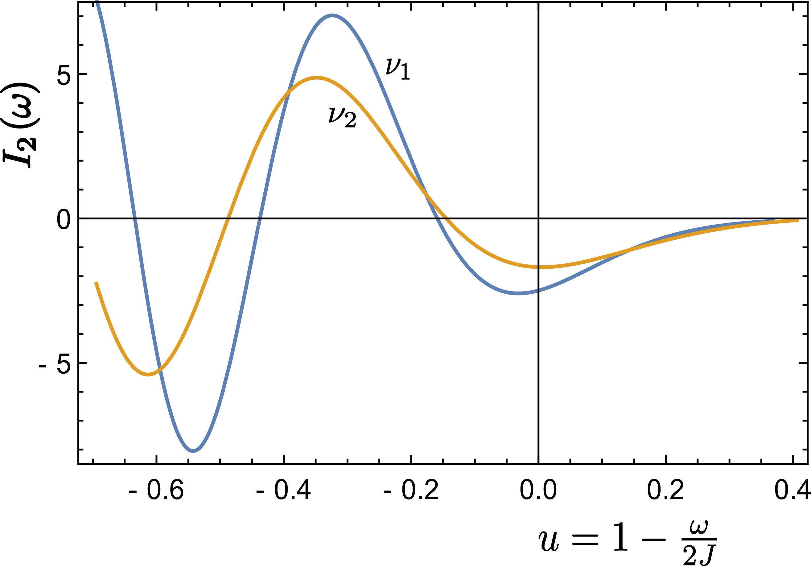 Figure 1
 Figure 2
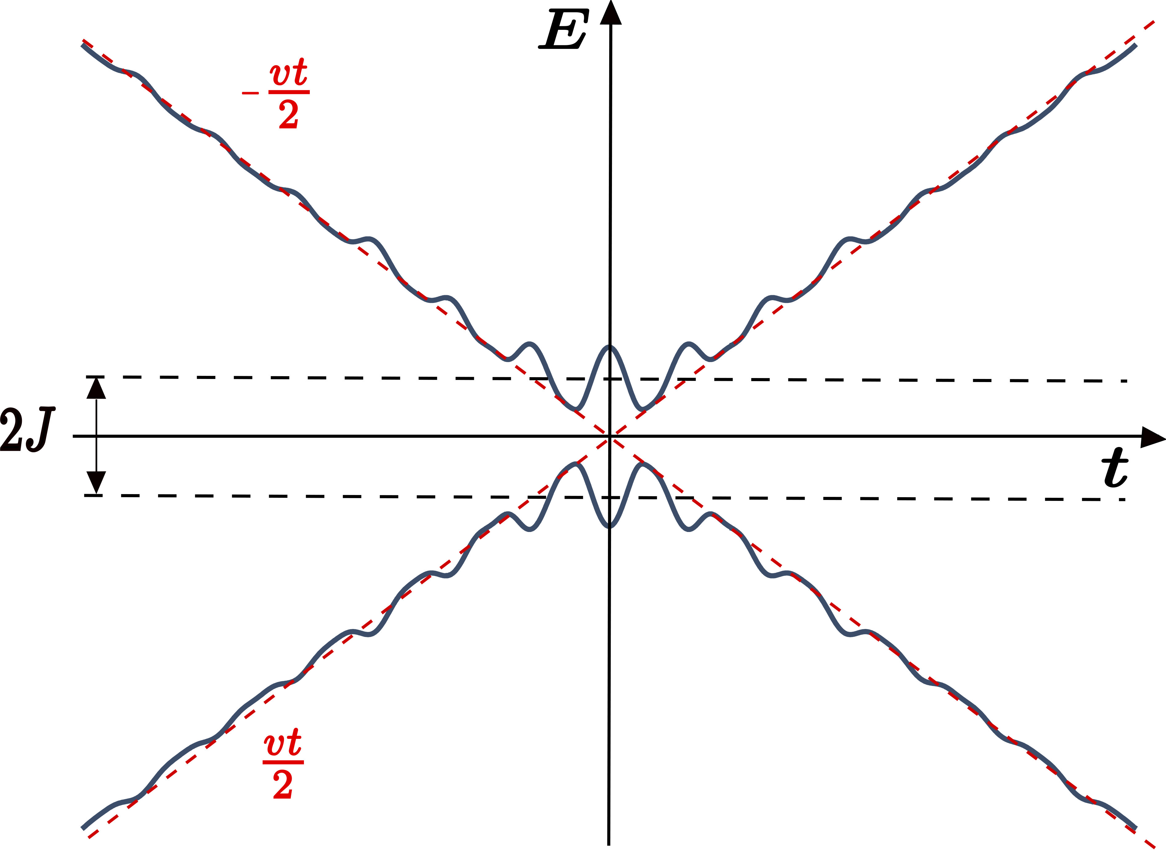 Figure 1
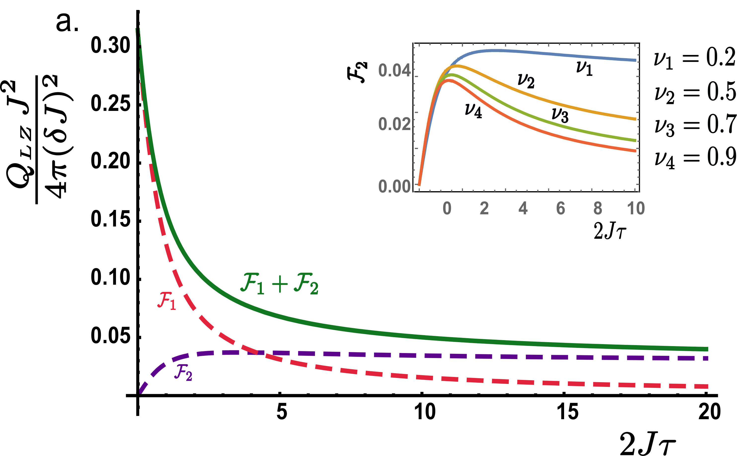 Figure 1
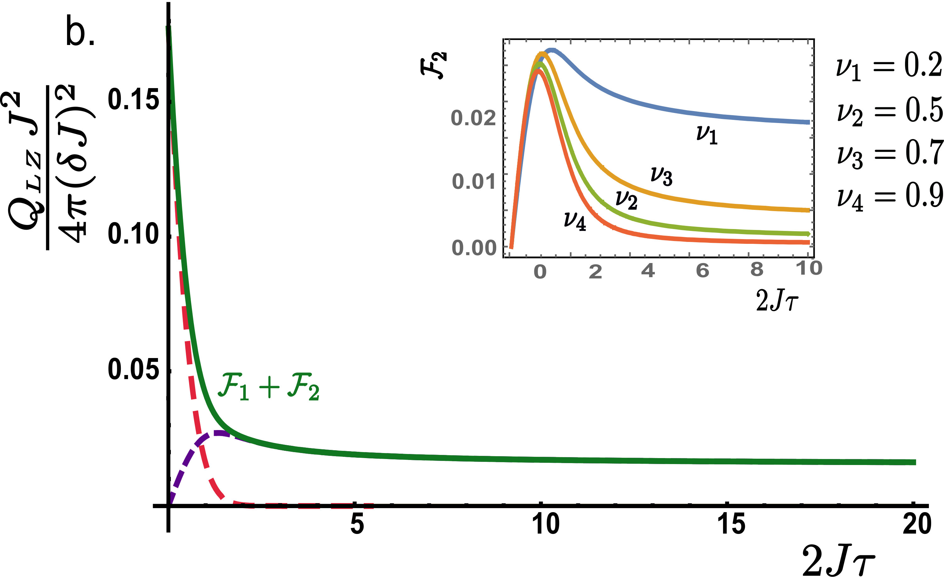 Figure 2
Peer Reviews
No public reviews on file for this paper yet. If you reviewed it on a platform where reviews are public (OpenReview, ICLR, NeurIPS, ICML), you can paste yours below so the community can read it here.
Videos
No videos yet. Explain this paper in a talk, walkthrough, or lecture? Add one.
Suppression of the Landau-Zener transition probability by a weak classical noise
Rajesh K. Malla, E. G. Mishchenko, and M. E. Raikh
Department of Physics and Astronomy, University of Utah, Salt Lake City, UT 84112
Abstract
When the drive which causes the level crossing in a qubit is slow, the probability, , of the Landau-Zener transition is close to . We show that in this regime, which is most promising for applications, the noise due to the coupling to the environment, reduces the average . At the same time, the survival probability, , which is exponentially small for a slow drive, can be completely dominated by noise-induced correction. Our main message is that the effect of a weak classical noise can be captured analytically by treating it as a perturbation in the Schrödinger equation. This allows us to study the dependence of the noise-induced correction to on the correlation time of the noise. As this correlation time exceeds the bare Landau-Zener transition time, the effect of noise becomes negligible. We consider two conventional realizations of noise: gaussian noise and telegraph noise.
pacs:
73.40.Gk, 05.40.Ca, 03.65.-w, 02.50.Ey
I Introduction
Theoretical papers on coherent manipulation of the quantum states of a qubit can be divided into two groups. At the focus of the first group, see e.g. Refs. Lim1991+++, ; Garanin2002+++, ; Berry2009+++, ; Bason2012+++, ; delCampo2013+++, ; Zhang2013+++, ; Ban2014+++, ; Polleti2016+++, ; Funo2017+++, , is a quest for “superadiabaticity”, which is an optimal protocol of drive-induced crossing of the energy levels. Following this protocol, at the end of the evolution, the final state of a qubit is as close as possible to the adiabatic ground state. If the time variation of the energy levels is linear, , where is the drive velocity, the degree of adiabaticity is given by the celebrated Landau-Zener (LZ) formulaLandau1932 ; Zener1932
[TABLE]
where is the tunnel splitting of the levels at the crossing point. The meaning of is the probability to find the system, which is in state at , in the state at . Correspondingly, the meaning of is the “survival” probability to find the system in the initial state.
The value serves as an estimate of the degree of adiabaticity achievable when a two-level system is forced through an avoided crossing. In this regard, “superadiabatic” protocol minimizes the survival probability.
In the papers of the second group, see e.g. Refs. [Galperin2008+, ; Nalbach2009+, ; Pekola2011+, ; Ziman2011+, ; Vavilov2014+, ; Nalbach2014+, ; Nalbach2015+, ; Ogawa2017+, ], the drive is assumed to be strictly linear. The subject of study is the effect of coupling of the qubit levels to the environment on the probability of the Landau-Zener transition.
A common approach to the study of the effect of environment (thermal bath) on the LZ transition is to add to the Hamiltonian of the two-level system the Hamiltonian of the bath and the Hamiltonian of the linear coupling of the bath to the two-level system. After that, the equations of motion for the density matrix are cast in the form of master equations. This is achieved by generalizing the Lindblad approach of Bloch-Redfield approach developed for stationary two-level systems to the case of time-dependent Hamiltonian. The resulting closed system of master equations is solved numerically.Galperin2008+ ; Nalbach2009+ ; Pekola2011+ ; Ziman2011+ ; Vavilov2014+ ; Nalbach2014+ ; Nalbach2015+ ; Ogawa2017+ This numerics sometimes reveals a peculiar dependenceZiman2011+ of the dynamics of the LZ transition on the noise frequency and intensity or, more precisely, on temperature.
The message of the present paper is that the effect of a weak classical noise can be studied analytically by treating it as perturbation in the Schrödinger equation. This allows to study the dependence of the noise-induced correction to on the correlation time of the noise. The situation when this correction plays a crucial role is strong-coupling limit, , when the bare LZ transition probability is exponentially close to . In this limit, the bare survival probability, , is exponentially small. We will show that the correction to is negative and does not contain the exponential factor . Thus, even a weak noise can dominate . We analyze the noise-induced correction for the two realizations of the noise: gaussian noise and the telegraph noise.
II Perturbative solution of the Schrödinger equation in the presence of noise
Denote with , the amplitudes to find a driven system in the and states, respectively. In the presence of random , modeling the noise, these amplitudes satisfy the following system of equations
[TABLE]
In the absence of noise, two linearly independent solutions of the system Eq. (2) have the form
[TABLE]
[TABLE]
where is the parabolic cylinder functionBateman1955 of the argument, , defined as , while the index is given by
[TABLE]
The solution Eq. 3 satisfies the “right” initial condition , i.e. that the system is initially in the state .
In the presence of noise, we search for the corrections to the amplitudes, and , in the form of the linear combination
[TABLE]
Substituting this form into Eq. (2) and keeping only , in the terms proportional to we arrive to the following linear system of equations for and
[TABLE]
Taking into account the initial conditions and , we find the expressions for and
[TABLE]
It is easy to see that the denominator in Eqs. (8), (9) is a time independent constant. This is the consequence of the relation
[TABLE]
which straightforwardly follows from the system Eq. (2). The expression in the right-hand side is a Wronskian, the value of which is knownBateman1955
[TABLE]
Here is the Gamma-function.
The exact expression for the survival probability is . Using Eq. (6), we can express this probability, with noise taken into account to the lowest order, via the bare survival probability as follows
[TABLE]
The latter expression illustrates our main point, namely, when the bare survival probability is exponentially small, the net survival probability is dominated by the noise-induced correction, . The analytical expression for this correction follows from Eq. (9). It should be averaged over the noise realizations. This averaging is carried out in the next Section.
III Averaging over the noise realizations
The strength and the correlation time of the noise are encoded in the correlator defined as
[TABLE]
where is the r.m.s. noise magnitude and .
Using Eqs. (10), and (11), the average survival probability, , can be expressed via the correlator as follows
[TABLE]
where we used the identity .
To evaluate the double integral, we take advantage of the fact that, without noise, the transition probability is close to , which implies that the parameter is big, . This, in turn, justifies using the semiclassical asymptotes for the parabolic cylinder functions not only for big, but, in fact, for all values of the argument. The asymptotic forms of the parabolic cylinder functions valid at large and arbitrary can be found in Ref. Luo2017, . Using these asymptotes, for the combination \Big{[}a_{\scriptscriptstyle\downarrow}^{\scriptscriptstyle(1)}(t)\Big{]}^{2}-\Big{[}a_{\scriptscriptstyle\uparrow}^{\scriptscriptstyle(1)}(t)\Big{]}^{2} which enters into Eq. (14), one obtains
[TABLE]
where is the semiclassical phase
[TABLE]
Due to being large, the term corresponding to in Eq. (15) is exponentially suppressed. The denominator in the prefactor is conventional for semiclassics. Appearance of in the numerator can be simply illustrated by substituting into the system Eq. (2). This will yield the relation
[TABLE]
For the further evaluation of the double integral in Eq. (14), it is convenient to switch from time domain to the frequency domain, as it is illustrated in the next section.
IV Calculation of in the frequency domain
Denote with the Fourier transform of the correlator Eq. (13)
[TABLE]
Upon substituting Eq. (18) into Eq. (14), the integrations over and get decoupled and we obtain
[TABLE]
where is given by
[TABLE]
Analytical form of depends on the frequency domain. For high one can use the steepest descent method. The exponent in Eq. (20) has two extrema at , where
[TABLE]
Expanding the exponent near these extrema and taking into account that , after combining the two contributions, we obtain
[TABLE]
The above result applies when the argument of sine is big. For this requirement is already satisfied when exceeds only slightly. Indeed, the criterion can be cast in the form
[TABLE]
Physically, this criterion means that the direct absorption (emission) of a noise “quantum”, say, a phonon, if the noise is due to lattice vibrations, is allowed.
For frequencies the behavior of exhibits a sharp cutoff as the difference grows. It appears that, in order to capture this cutoff, it is sufficient to replace by its small- expansion, namely
[TABLE]
One can also neglect in the denominator of Eq. (20 ). After that, reduces to the derivative of the Airy function, namely
[TABLE]
The behavior of near is illustrated in Fig. 2. For it falls off exponentially as
\exp\Big{[}-\frac{2^{7/2}|\nu|}{3}(1-\omega/2J)^{3/2}\Big{]} when exceeds , while for it oscillates and reduces to the asymptote Eq. (22) after the first maximum. It follows from the plot that, numerically, the small- tail is relatively slim. Still, we will keep it, since it captures for long correlation times of the noise. For arbitrary correlation time, it is sufficient to use the asymptote Eq. (22) for and the asymptote Eq. (25) for . Then the expression Eq. (19) for the average survival probability takes the form
[TABLE]
where we have replaced by , since is big. Eq. (26) is our main result. While the dependence of on the on the noise magnitude is obvious, the dependence on the noise correlation time, predicted by Eq. (26) is nontrivial. We analyze this dependence in the next section.
V Dependence of on the noise correlation time
If the correlation time of the noise is , then is a dimensionless function of the argument . Since the frequency scale of both and is the gap , the two contributions to are the dimensionless functions of the argument . Correspondingly, we rewrite Eq. (26) in the form
[TABLE]
where the functions and are defined as
[TABLE]
[TABLE]
The first and the second terms describe the absorption of “above-gap” and “below-gap” noise quanta, respectively. Note, that the integrand in Eq. (28) does not contain the parameter . In Fig. 3(a),(b) we plotted for the telegraph noise with and for the gaussian noise with , respectively. The contributions can be evaluated analytically for both cases. Namely, for the telegraph noise the calculation yields
[TABLE]
while for gaussian noise the result reads
[TABLE]
where is the error function. The contributions dominate in the small- domain, which corresponds to the fast noise. In fact, the contribution turns to zero for . The behavior of the contributions at small is for the telegraph noise and {\cal F}_{2}(2J\tau)\approx|\nu|\bigl{(}\frac{\pi^{1/2}}{2}-2J\tau\bigr{)} for the gaussian noise. The slopes are related as , i.e. they are close. The fact that for short correlations times the prefactor in is proportional to reflects a simple physics that the absorption of the high-frequency noise quanta does not depend on . Indeed, drops out from the combination .
The difference between the two noise realizations manifests itself in the contributions . It is seen from Fig. 3 that for the telegraph noise, this contribution falls off with much slower than for the gaussian noise. In fact, the slow decay of can be estimated qualitativelyLuo2017 . Indeed, subsequent jumps of the gap width with magnitude take place at time moments, , separated by . A jump results in the absorption only if , since is the LZ transition time. The probability that is . This suggests that contribution falls off as . A nontrivial feature of the contribution is that it passes through a maximum at .
VI Longitudinal noise
Throughout the paper we assumed that the noise is transverse, i.e. it is described by the Hamiltonian . In this section we briefly outline the changes to be made in the result Eq. (27) if the noise is longitudinal with the Hamiltonian . The steps of the perturbative derivation of leading to Eq. (14) for the longitudinal noise are completely similar to the transverse noise. Naturally, instead of appears in the prefactor. In the integrand, the combination \Big{[}a_{\scriptscriptstyle\downarrow}^{\scriptscriptstyle(1)}(t_{1})\Big{]}^{2}-\Big{[}a_{\scriptscriptstyle\uparrow}^{\scriptscriptstyle(1)}(t_{1})\Big{]}^{2} gets replaced by 2\Big{[}a_{\scriptscriptstyle\downarrow}^{\scriptscriptstyle(1)}(t_{1})a_{\scriptscriptstyle\uparrow}^{\scriptscriptstyle(1)}(t_{1})\Big{]}. The absolute value of the former combination has a meaning of , which is the absolute value of the polarization. Correspondingly, the absolute value of the product 2\Big{[}a_{\scriptscriptstyle\downarrow}^{\scriptscriptstyle(1)}(t_{1})a_{\scriptscriptstyle\uparrow}^{\scriptscriptstyle(1)}(t_{1})\Big{]} corresponds to . For , this quantity is calculated in the Appendix. Then the modification of Eq. (20) amounts to the replacement of by in the numerator of the integrand. As a result, for the result Eq. (22) gets modified as
[TABLE]
Due to this modification, the integral in the expression for the survival probability assumes the form
[TABLE]
For the telegraph noise, the evaluation of this integral yields
[TABLE]
We see that the result differs from the corresponding expression Eq. (30) only by an additional factor in the square brackets. We conclude that the effect of longitudinal noise on is suppressed, compared to the transverse noise, in the limit , i.e. in the limit of the fast noise.
VII Discussion
In this section we compare our results with the results of previous studiesNalbach2009+ ; Nalbach2014+ ; Nalbach2015+ ; Wubs2006++ ; Pokrovsky2007++ ; Wubs2007++ ; Ao1991 of the effect of noise on the LZ transition.
(i). We calculated the survival probability for arbitrary noise correlation time assuming that the noise is weak, so that the bare survival probability is exponentially small. This domain of parameters corresponds to “high-fidelity” qubit and is most appealing for applications. In earlier analytical calculations Refs. Wubs2006++, ; Pokrovsky2007++, ; Wubs2007++, the noise intensity was not assumed to be weak, but the the noise was assumed to be fast. Both longitudinal and transverse noise were treated on the same footing. The authors adopted a standard model of a bosonic bath consisting of harmonic oscillators. For the case of transverse noise (affecting only ) considered in the present paper the results of Refs. Wubs2006++, ; Pokrovsky2007++, ; Wubs2007++, can be summarized as follows. In the presence of noise Q_{\scriptscriptstyle LZ}=\exp\Big{[}-2\pi(J^{2}+(\delta J)^{2})/v\Big{]}, which suggests that the noise suppresses the survival probability in contrast to what we find. This conclusion was questioned in subsequent detailed numerical studies.Nalbach2009+ ; Nalbach2014+ ; Nalbach2015+ The results of Refs. Nalbach2009+, , Nalbach2014+, , and Nalbach2015+, demonstrate that the Landau-Zener probability decreases with temperature, i.e. with noise magnitude, for all values of the bare LZ probability (all values of parameter ). An interesting observation made in these papers is that , modified by noise, is a non-monotonic function of .
(ii). Technically, our calculation is most close to the paper by Ao and Rammer Ref. Ao1991, . In our notations and, within a numerical factor, their result reads, , where is the Bose distribution. The above expression suggests that the noise-induced survival probability is dominated exclusively by the noise “quanta” with frequency . This conclusion seems unphysical and contradicts our result Eq. (26), according to which all frequencies with contribute to . On the quantitative level, the difference can be traced to the use of the asymptotes of the parabolic cylinder functions in Ref. Ao1991, .
(iii). Note finally, that for very strong noise the LZ transition can be viewed as simply noise-driven. This limit was studied in a pioneering paper Ref. Kayanuma1985, . In particular, for fast noise, with frequency much bigger than , the survival probability is given by Q_{\scriptscriptstyle LZ}=\frac{1}{2}\Big{[}1+\exp\left(-4\pi(\delta J)^{2}/v\right)\Big{]}.
(iv). Throughout the paper we assumed that is big, i.e. the bare survival probability is small. It is interesting to note that, in the opposite limit of small enough , the dependence of survival probability on the noise magnitude can be non-monotonic. Below we illustrate this observation analytically assuming that the noise is slow.
It is knownKayanuma1985 that in the limit of infinite , the average probability of the transition should be calculated by averaging this probability of transition at a given over the distribution of .
For slow noise with correlation time much longer than , the survival probability is given by
[TABLE]
For gaussian P\left(\delta J\right)=\frac{1}{\pi^{1/2}J_{0}}\exp\big{[}-\left(\frac{\delta J}{J_{0}}\right)\big{]}^{2} the integration yields
[TABLE]
Note that, for , the survival probability is suppressed by noise while for it is enhanced by noise. This behavior is illustrated in Fig. 4. Fig. 4 suggests the following nontrivial effect of low-frequency environmentZiman2011+ on the LZ transition. As the coupling to environment, parametrized by , increases, the initially adiabatic transition becomes first less adiabatic, and then, more adiabatic.
(v). The noise spectrum, , depends on the concrete realization of the environment. In theoretical papers, see e.g. Refs. Nalbach2009+, , Nalbach2014+, , Nalbach2015+, , the environment is usually modeled by a set of harmonic oscillators with the frequency distribution (Ohmic environment). Then is proportional to , where is temperature.
Appendix A Time evolution of the level population in the limit of small survival probability
In general, the level populations, and exhibit strong oscillations in the domain , where the LZ transition takes place. These oscillations originate from the interference of the terms and , Eq. (16). The reason why we were able to find the noise-dependent correction analytically is that, for small bare survival probability, these oscillations are suppressed. We established this fact upon analysis of the asymptotes of the parabolic cylinder functions in the domain . It is instructive to trace how the result Eq. (15)
[TABLE]
emerges from the alternative description based on the spin dynamics. In the literature, the effect of noise on the LZ transition is studied within this description.
The difference can be viewed as spin polarization, while the system Eq. (2) describes the evolution of the and spin amplitudes in the effective magnetic field, , with components and . Three equations of motion for the spin projections following from can be reduced to a single integral-differential equation for
[TABLE]
The crucial simplification, which allows to solve this equation in the limit is that, for relevant times , the argument of cosine is big. For , Eq. (38) takes the form
[TABLE]
Strong oscillations of cosine suggest that the major contribution to the integral comes from . To make use of this condition, we perform the integration by parts in the right-hand side
[TABLE]
Next, we set in the argument of sine and set in the derivative. This yields
[TABLE]
Now the integration over can be carried out leading to
[TABLE]
The first order differential equation Eq. (42) can be easily solved. With initial condition , the result reads
[TABLE]
i.e. the polarization is equal to cosine of the angle between magnetic field and the -axis. Using Eq. (43), the projection can be calculated from the equation and turns out to be
[TABLE]
Subsequently, the projection calculated from acquires the form
[TABLE]
From the expressions Eqs. (43)-(45), we can estimate the accuracy of the approximations made. These expressions are valid if . Indeed, it follows from (43), (45) that . On the other hand, it follows from Eq. (44) that the maximal value of is . Thus, the results Eqs. (43)-(45) are valid with accuracy . Uncertainty is much bigger than the inaccuracy of the result , which follows from Eq. (43). Inaccuracy of this result is , i.e. it is exponentially small.
Numerical results for the spin projections in the limit are presented in Ref. Ziman2011+, . They seem to be in good agreement with analytical expressions Eqs. (43)-(45).
Acknowledgements
Illuminating discussion with V. L. Pokrovsky is gratefully acknowkedged. The work was supported by the Department of Energy, Office of Basic Energy Sciences, Grant No. DE- FG02-06ER46313.
The reference list from the paper itself. Each links out to its DOI / PubMed record.
- 1(1) R. Lim and M. V. Berry, “Superadiabatic tracking of quantum evolution,” J. Phys. A Math. Gen. 24 , 3255 (1991).
- 2(2) D. A. Garanin and R. Schilling, “Inverse problem for the Landau-Zener effect,” Europhys. Lett. 59 , 7 (2002).
- 3(3) M. V. Berry, “Transitionless quantum driving,” J. Phys. A: Math. Theor. 42 , 365303 (2009).
- 4(4) M. G. Bason, M. Viteau, N. Malossi, P. Huillery, E. Arimondo, D. Ciampini, R. Fazio, V. Giovannetti, R. Mannella, and O. Morsch “ High-fidelity quantum driving,” Nat. Phys. 8 , 147 (2012).
- 5(5) A. del Campo, “Shortcuts to Adiabaticity by Counterdiabatic Driving,” PRL 111 , 100502 (2013).
- 6(6) Z. Zhang and Y. Yu, “Processing quantum information in a hybrid topological qubit and superconducting flux qubit system,” Phys. Rev. A 87 , 032327 (2013).
- 7(7) Y. Ban and X. Chen, “Counter-diabatic driving for fast spin control in a two-electron double quantum dot,” Sci. Reports 4 , 6258 (2014).
- 8(8) Z. Sun, L. Zhou, G. Xiao, D. Poletti, and J. Gong, “Finite-time Landau-Zener processes and counterdiabatic driving in open systems: Beyond Born, Markov, and rotating-wave approximations,” Phys. Rev. A 93 , 012121 (2016).