Constraint Energy Minimizing Generalized Multiscale Finite Element Method in the Mixed Formulation
Eric Chung, Yalchin Efendiev, Wing Tat Leung

TL;DR
This paper introduces a mass-conservative mixed multiscale finite element method for flow in heterogeneous porous media, achieving contrast-independent first-order convergence by constructing specialized basis functions.
Contribution
It develops a novel multiscale method with auxiliary spaces and local basis functions that ensure contrast-independent accuracy in heterogeneous media.
Findings
First-order convergence rate achieved
Convergence independent of media contrast
Method effectively captures high-conductivity channels
Abstract
This paper presents a novel mass-conservative mixed multiscale method for solving flow equations in heterogeneous porous media. The media properties (the permeability) contain multiple scales and high contrast. The proposed method solves the flow equation in a mixed formulation on a coarse grid by constructing multiscale basis functions. The resulting velocity field is mass conservative on the fine grid. Our main goal is to obtain first-order convergence in terms of the mesh size which is independent of local contrast. This is achieved, first, by constructing some auxiliary spaces, which contain global information that can not be localized, in general. This is built on our previous work on the Generalized Multiscale Finite Element Method (GMsFEM). In the auxiliary space, multiscale basis functions corresponding to small (contrast-dependent) eigenvalues are selected. These basis…
Click any figure to enlarge with its caption.
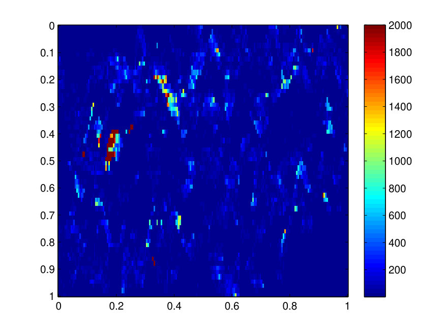 Figure 1
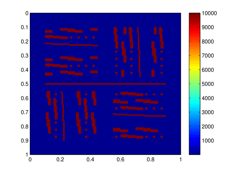 Figure 2
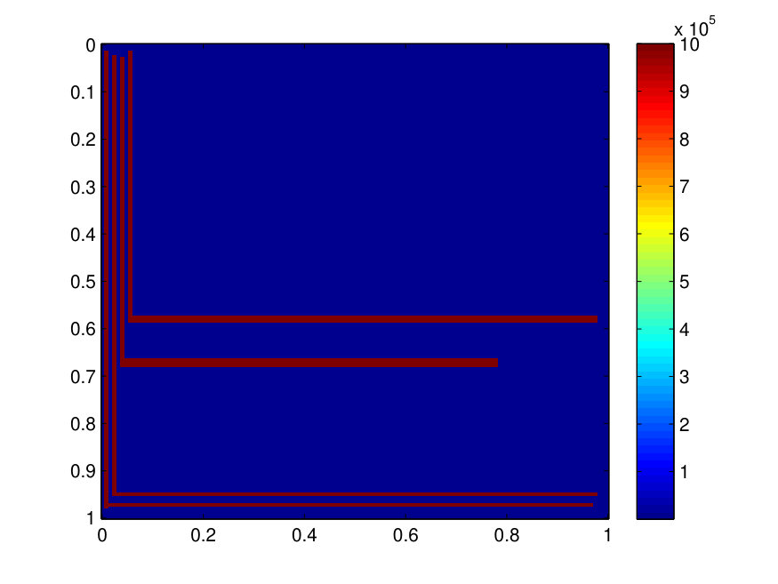 Figure 3
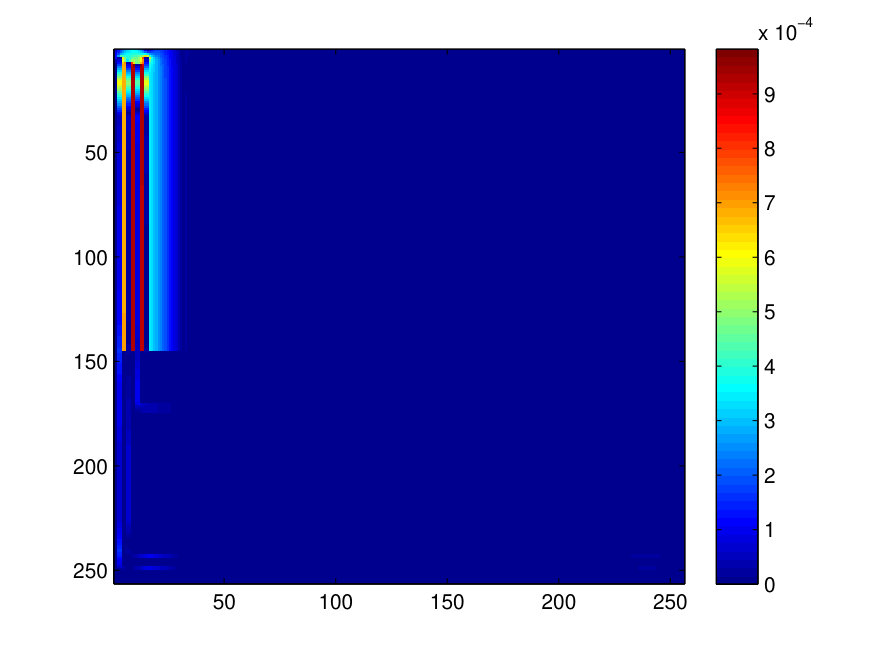 Figure 4
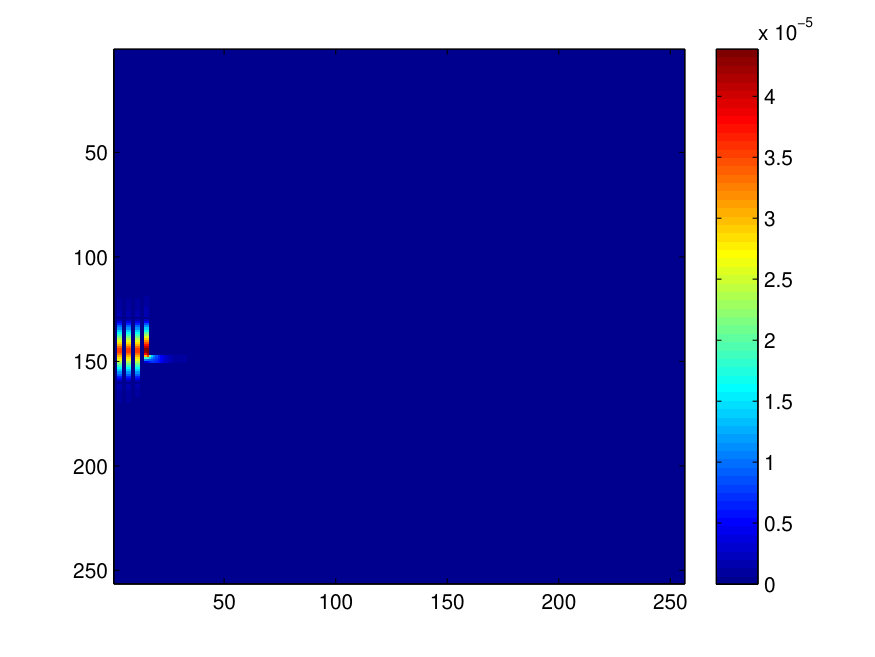 Figure 5
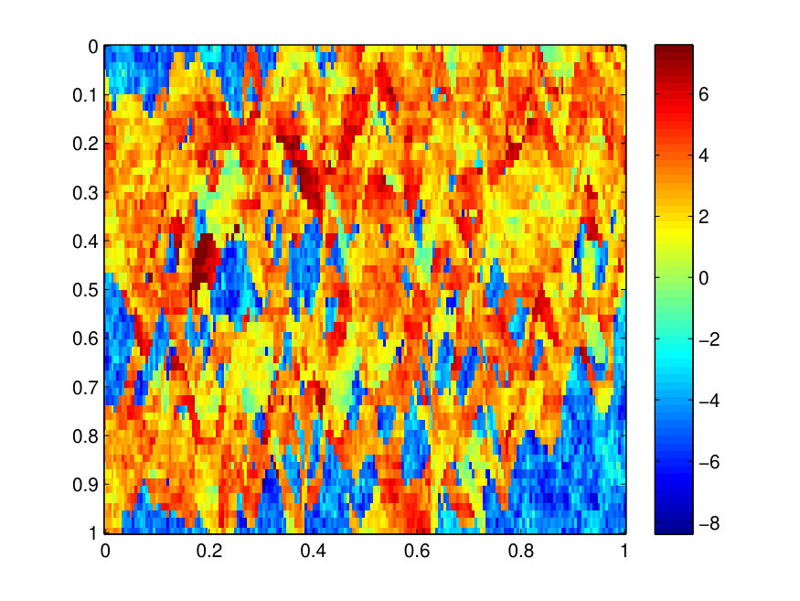 Figure 6
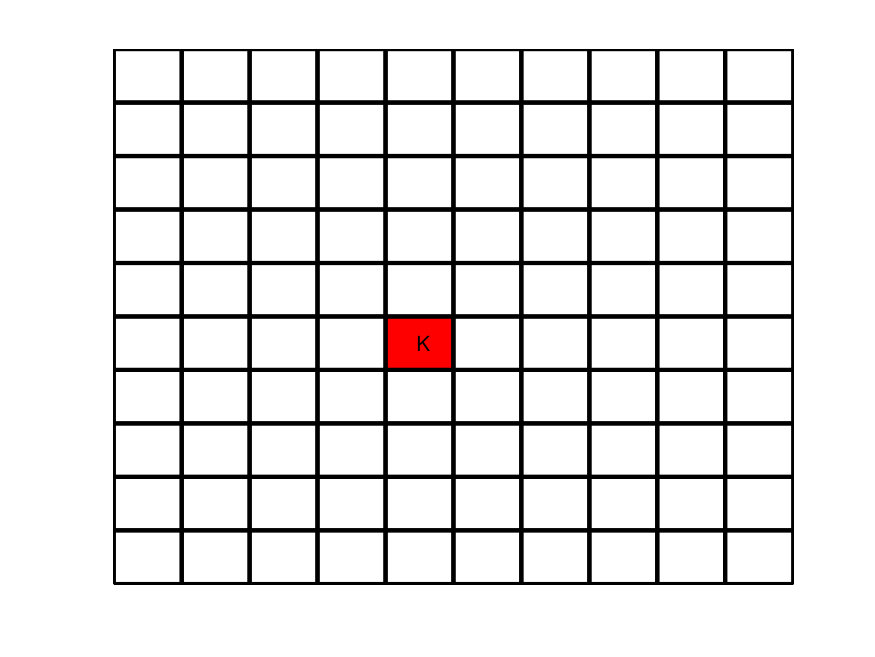 Figure 7
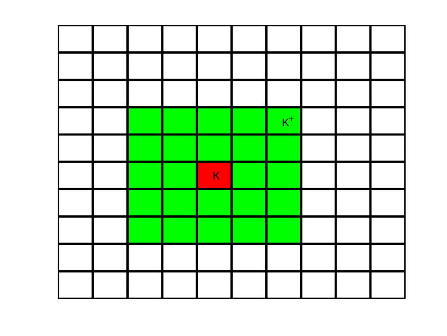 Figure 8
| Number basis per element | H | # oversampling coarse layers | ||
|---|---|---|---|---|
| 3 | 1/8 | 3 | 12.2392% | 3.4897% |
| 3 | 1/16 | 4 | 2.7549% | 0.9931% |
| 3 | 1/32 | 5 | 0.8292% | 0.3227% |
| 3 | 1/64 | 6 | 0.2811% | 0.1098% |
| Number basis per element | H | # oversampling coarse layers | ||
|---|---|---|---|---|
| 1 | 1/8 | 3 | 28.5354% | 75.6655% |
| 1 | 1/16 | 4 | 12.5646% | 18.2546% |
| 1 | 1/32 | 5 | 5.6206% | 3.0618% |
| 1 | 1/64 | 6 | 2.3959% | 0.8156% |
| Number basis per element | H | # oversampling coarse layers | ||
|---|---|---|---|---|
| 4 | 1/8 | 3 | 58.8673% | 67.3385% |
| 4 | 1/16 | 4 | 7.5104% | 17.9436% |
| 4 | 1/32 | 5 | 2.5633% | 6.5846% |
| 4 | 1/64 | 6 | 0.7907% | 1.9459% |
| Number basis per element | H | # oversampling coarse layers | ||
|---|---|---|---|---|
| 1 | 1/8 | 3 | 86.5779% | 105.0276% |
| 1 | 1/16 | 4 | 211.2798% | 89.6828% |
| 1 | 1/32 | 5 | 44.3964% | 50.7899% |
| 1 | 1/64 | 6 | 6.4084% | 8.3319% |
| Number basis per element | H | # oversampling coarse layers | ||
|---|---|---|---|---|
| 4 | 1/10 | 3 | 8.5204% | 12.7005% |
| 4 | 1/20 | 4 (log(1/20)/log(1/10)*3=3.90) | 3.7952% | 7.2393% |
| 4 | 1/40 | 5 (log(1/40)/log(1/10)*3=4.8062) | 1.4931% | 4.2122% |
Peer Reviews
No public reviews on file for this paper yet. If you reviewed it on a platform where reviews are public (OpenReview, ICLR, NeurIPS, ICML), you can paste yours below so the community can read it here.
Videos
No videos yet. Explain this paper in a talk, walkthrough, or lecture? Add one.
Constraint Energy Minimizing Generalized Multiscale Finite Element Method
in the Mixed Formulation
Eric Chung Department of Mathematics, The Chinese University of Hong Kong (CUHK), Hong Kong SAR. Email: [email protected]. The research of Eric Chung is supported by Hong Kong RGC General Research Fund (Project 14317516).
Yalchin Efendiev Department of Mathematics & Institute for Scientific Computation (ISC), Texas A&M University, College Station, Texas, USA. Email: [email protected].
Wing Tat Leung Department of Mathematics, Texas A&M University, College Station, TX 77843
Abstract
This paper presents a novel mass-conservative mixed multiscale method for solving flow equations in heterogeneous porous media. The media properties (the permeability) contain multiple scales and high contrast. The proposed method solves the flow equation in a mixed formulation on a coarse grid by constructing multiscale basis functions. The resulting velocity field is mass conservative on the fine grid. Our main goal is to obtain first-order convergence in terms of the mesh size which is independent of local contrast. This is achieved, first, by constructing some auxiliary spaces, which contain global information that can not be localized, in general. This is built on our previous work on the Generalized Multiscale Finite Element Method (GMsFEM). In the auxiliary space, multiscale basis functions corresponding to small (contrast-dependent) eigenvalues are selected. These basis functions represent the high-conductivity channels (which connect the boundaries of a coarse block). Next, we solve local problems to construct multiscale basis functions for the velocity field. These local problems are formulated in the oversampled domain taking into account some constraints with respect to auxiliary spaces. The latter allows fast spatial decay of local solutions and, thus, allows taking smaller oversampled regions. The number of basis functions depends on small eigenvalues of the local spectral problems. Moreover, multiscale pressure basis functions are needed in constructing the velocity space. Our multiscale spaces have a minimal dimension, which is needed to avoid contrast-dependence in the convergence. The method’s convergence requires an oversampling of several layers. We present an analysis of our approach. Our numerical results confirm that the convergence rate is first order with respect to the mesh size and independent of the contrast.
1 Introduction
Multiscale problems occur in many subsurface applications. Multiple scales in permeabilities (subsurface properties) can span a large range and the variations in the permeability can be of several orders of magnitude. Moreover, the subsurface problems are often solved multiple times with different source terms and boundary conditions, e.g., in optimization of well locations. These models often admit a reduced representation and both local and global model reduction techniques have been developed in many papers. In local model reduction techniques, a reduced-order model on a coarse grid (with the grid size much larger than the heterogeneities) is sought. One of the commonly used methods includes upscaling of the permeability field [18, 9, 39]. This is done by solving local problems in each coarse block and computing the effective properties. Similar ideas have been employed for upscaling relative permeabilities in multi-phase flow simulations [5, 19]. The resulting effective medium is, then, used in a mass-conservative simulation.
An alternative approach to upscaling methods for simulations of single and multi-phase flows is the multiscale method [27, 24, 29, 23, 12, 30]. In multiscale methods, the local solutions on a coarse grid are used as basis functions in simulating flow equations. Because subsurface applications require mass conservative velocity fields, multiscale finite volume [30, 26, 32, 17, 31], mixed multiscale finite element methods [10, 1, 2, 3, 7, 8, 15], mortar multiscale methods [38, 4, 37, 14], and various post-processing methods are proposed to guarantee mass conservation [6, 34]. Obtaining a mass-conservative velocity in multiscale simulations requires special formulations.
One of the mass-conservative multiscale approaches that has been developed and widely used is based on a mixed finite element formulation [10, 1, 2, 3]. In a mixed formulation, the flow equation is formulated as two first-order equations for the pressure and velocity field. The multiscale basis functions are mainly sought for the velocity field, which is used to approximate the transport equations and requires mass conservation. Previous approaches developed multiscale basis functions for the velocity field using local solutions with Neumann boundary conditions and used piecewise constant basis functions for the pressure equations. In this case, support of the pressure basis function consists of a single coarse block, while support of the velocity basis functions consists of two coarse blocks that share a common face. These multiscale approaches have been widely developed in [10, 1, 2, 3] and applied to various multiphase applications. In these approaches, one multiscale basis function is computed for each edge (that two coarse blocks share) and spatially distributed fluxes on an internal face is imposed to reduce the subgrid effects.
In some recent works [12, 21], a Generalized Multiscale Finite Element Method has been proposed in a mixed formulation [16, 25]. In these papers, the multiscale basis functions for the velocity are computed, as before, in two coarse blocks that share a common face and the pressure basis functions are computed in each coarse block. The main difference compared to previous approaches is that a systematic approach is designed to compute multiple velocity basis functions. These velocity basis functions are computed by constructing the snapshot spaces in two coarse-block regions and then solving local spectral problems in the snapshot spaces. The typical snapshot functions consist of local solutions with prescribed Neumann boundary conditions on the common interface between two coarse blocks. The local spectral decomposition (based on the analysis) identifies appropriate local spaces. In particular, by ordering the eigenvalues in increasing order, we select the eigenvectors corresponding to small eigenvalues. The convergence analysis of these approaches is performed in [16], which shows a spectral convergence , where is the smallest eigenvalue corresponding to the eigenvector that is not included in the coarse space. However, this convergence estimate does not include a coarse-mesh dependent convergence. The latter is our goal in this paper.
This paper follows some of the main concepts developed in [13] to design a mixed multiscale method, which has a convergence rate proportional to , where is the coarse-mesh size and is the smallest eigenvalue that the corresponding eigenvector is not included in the coarse spaces. To obtain first order convergence in terms of the coarse-mesh size, we use some ideas from [36, 33, 35, 28]. The proposed approach requires some oversampling and a special basis construction. Our approach and the analysis significantly differ from our earlier work [13], where we designed a continuous Galerkin technique. Moreover, the proposed method provides a mass conservative velocity field. Because of the high-contrast in the permeability field, we first need to identify non-local information that depends on the contrast. This is done by solving local spectral problems for the pressure field and Constructing an auxiliary space. The auxiliary space contains non-local information represented by channels (high-conductivity regions that connect the boundaries of the coarse block). It is important to separately include this information in the coarse space (e.g., [20, 22]). To construct multiscale basis functions, we solve local problems in a large oversampled region with an appropriate orthogonality condition. The latter allows fast decay of the “remaining” information and takes into account the non-decaying part of the local solution in the oversampled domain. The proposed method provides a convergence rate under certain conditions on the oversampled region. Here is the minimal eigenvalue as discussed above.
We present numerical results and consider three permeability fields. In the first two cases, the permeability fields have distinct channels and the number of channels are selected to have a certain number of minimum basis functions in each coarse block. Our numerical results show that with an appropriate number of basis functions, we can achieve first-order convergence with respect to the coarse-mesh size. In our third numerical example, we consider SPE 10 Benchmark tests [11]. In this case, the number of channels is not explicitly identified and we use an auxiliary space with several basis functions. Our numerical results show that one can achieve less than % error in the velocity field using four dimensional auxiliary space and oversampling.
The paper is organized as follows. In Section 2, we present some preliminaries and discuss coarse and fine grids. Section 3 is devoted to describing the multiscale method. The analysis is presented in Section 4. We present the numerical results in Section 5.
2 Preliminaries
Motivated by the importance of mass conservation for flow problems in heterogeneous media, we consider a class of high-contrast flow problems in the following mixed form
[TABLE]
subject to the homogeneous boundary condition on , where is the computational domain, is the dimension and is the outward unit normal vector on . Note that the source function satisfies . We assume that is a heterogeneous coefficient with multiple scales and very high contrast. We assume that , where is large. Let and . We define . Then we can formulate the problem (1) in the following weak formulation: find and such that
[TABLE]
where
[TABLE]
We remark that the above problem (2) is solved together with the condition . We also remark that the following inf-sup condition holds: for all with , we have
[TABLE]
where is independent of .
We next introduce the notion of fine and coarse grids. We let be a usual conforming partition of the computational domain into finite elements (triangles, quadrilaterals, tetrahedra, etc.). We refer to this partition as the coarse grid and assume that each coarse element is partitioned into a connected union of fine grid blocks, see Figure 1, where a coarse mesh is shown. The fine grid partition will be denoted by , and is by definition a refinement of the coarse grid . We let be the number of coarse elements and let be the number of coarse grid nodes of . We remark that our basis functions are constructed based on the coarse mesh. In order to compute numerically the basis functions on coarse elements, we need the underlying fine mesh. In the next section, we will discuss in detail the construction of basis functions.
3 The Multiscale Method
In this section, we will present the construction of our method. The construction consists of two general steps. In the first step, we will construct a multiscale space for the pressure . In the second step, we will use the multiscale space for pressure to construct a multiscale space for the velocity . We remark that the basis functions for pressure are local, that is, the supports of pressure basis are the coarse elements. On the other hand, for each pressure basis function, we will construct a related velocity basis function, whose support is an oversampled region containing the support of the pressure basis functions. This oversampled region is usually obtained by enlarging a coarse element by several coarse grid layers, see Figure 1. This localized feature of the velocity basis function is the key to our method.
3.1 Pressure basis functions
In this section, we will present the construction of the pressure multiscale basis functions. We will construct a set of auxiliary multiscale basis functions for each coarse element using a spectral problem. First we define some notations. For a general set , we define , and . Next, we define the required spectral problem. For each coarse element , we solve the eigenvalue problem: find and such that
[TABLE]
where
[TABLE]
and is the set of standard multiscale basis functions, which satisfy the partition of unity property. One can also use other types of partition of unity functions, for example, the set of standard bilinear basis functions. Assume that and that we arrange the eigenvalues of (5) in non-decreasing order . To define the required multiscale basis functions, we pick the first eigenfunctions and define the local auxiliary multiscale finite element space by
[TABLE]
The (global) auxiliary multiscale finite element space is defined by . Notice that, the space will be used as the approximation space for the pressure.
3.2 Velocity basis functions
In this section, we will present the construction of the velocity basis functions. For each of the pressure basis function in , we will construct a corresponding velocity basis function, whose support is an oversampled region containing the support of the pressure basis function (see Figure 1).
First of all, we define the interpolation operator by
[TABLE]
Note that is the projection of onto with respect to the inner product , where is defined in (6).
Next, we give two types of velocity multiscale basis functions. These two types are motivated by the two types of constructions as in [13]. Let be a given pressure basis function supported in . We let be the corresponding oversampled region, see Figure 1. We will define a velocity basis function by solving the following problem. The multiscale space is defined as . Note that the basis function is supported in , which is a union of connected coarse elements and contains . We define as the set of indices such that if , then . We also define .
- •
Type 1 basis functions
We find , and such that
[TABLE]
- •
Type 2 basis functions
We find and such that
[TABLE]
We remark that the Type 1 basis functions are motivated by the constraint energy minimization problem defined in [13] (more precisely, equation (7) in [13]). One can show that the variational formulation of the corresponding mixed formulation of the minimization problem is exactly given by (7)-(9). The Type 2 basis functions are motivated by the unconstraint energy minimization problem in [13] (more precisely, equation (24) in [13]). One can show that the variational formulation of the corresponding mixed formulation of the minimization problem is exactly given by (10)-(11).
In the following, we will consider only the Type 2 basis functions, due to its better performance as shown in [13]. Notice that, we can define the basis function in the local region is because of a localization property of the related global basis function . The global basis function is constructed by solving the following problem. The global multiscale space is defined as .
- •
Type 2 basis functions (global)
We find and such that
[TABLE]
Notice that the system (12)-(13) defines a mapping from to . In particular, given , the image is defined by
[TABLE]
We remark that the mapping is surjective.
Next, we give a characterization of the space in the following lemma.
Lemma 1**.**
Let be the global multiscale space for the velocity. For each with , there is a unique such that is the solution of
[TABLE]
and .
Proof.
We define the space using the following construction. We can define a mapping using the system (16), and then define as the image of this map. It suffices to show that .
It is clear that . By the construction of the above map, we have . Thus, we will prove next that . To do so, we will show that the null space of the mapping has dimension one. Assume that is in the null space of . Let and . By definition of ,
[TABLE]
By assumption, . By (17), we have
[TABLE]
Since , we have
[TABLE]
where is the mean value of . By the inf-sup condition 4, we conclude that , which implies that is a constant function. Using (18) and contains constant functions, we have
[TABLE]
Thus, is a constant function. Therefore, we conclude that the dimension of the null space of is one.
∎
3.3 The method
From the above, we have the multiscale spaces and for the approximation of pressure and velocity. The multiscale solution is obtained by solving
[TABLE]
To analyze the method, we will first define some norms for our spaces. We define the norms and for by
[TABLE]
Next, we define a norm for the space by
[TABLE]
For a given subregion , we will define a local version of the norms , and by
[TABLE]
Finally, denotes the standard norm on .
4 Analysis
The analysis consists of several steps. In Section 4.1, we will analyze the stability and the convergence of using the global basis functions. Then in Section 4.2, we will analyze the well-posedness of the construction of the multiscale basis functions. We will in Section 4.3 prove a decay property of the global multiscale basis functions, and justify the localization procedure. Finally, in Section 4.4, we will analyze the stability and the convergence of using the multiscale basis functions.
For our analysis, we define
[TABLE]
Moreover, we define the snapshot solution by
[TABLE]
The well-posedness of (21)-(22) is standard. Note that for all . We remark that is considered as the reference solution is our analysis, and we will estimate the differences and . In the following lemma, we will show that the differences and are small. That is, the snapshot error is small.
Lemma 2**.**
Let be the snapshot solution defined in (21)-(22) and let be the exact solution defined in (2). Then we have
[TABLE]
In addition, we have
[TABLE]
Proof.
First, we have
[TABLE]
Taking and in the above system, and summing the two equations, we have
[TABLE]
For each coarse element , we define be the restriction of on . Then, by the definition of , we can write
[TABLE]
We define as
[TABLE]
Letting in the first equation of (25), we have
[TABLE]
Using the spectral problem (5), we have
[TABLE]
In addition, we have . Then using (5), we have
[TABLE]
Combining the above results, we obtain
[TABLE]
Hence we proved (23).
Using the inf-sup condition (4) and (25), we have
[TABLE]
This proves (23).
Finally, using (26), we have
[TABLE]
This proves (24).
∎
The above lemma shows that, when the partition of unity functions is chosen as the standard piecewise bilinear functions, we obtain the convergence rate , which is independent of the contrast.
4.1 Stability and convergence of using global basis functions
In this section, we consider the use of the global basis functions to solve the problem. In particular, we approximate the problem (1) using the space for pressure and for velocity. So, we define the solution using global basis function by the following
[TABLE]
Note that for all . We will prove the stability and the convergence of (28)-(29).
First, we prove the following inf-sup condition.
Lemma 3**.**
For every with , there is such that
[TABLE]
Proof.
Let with . Similar to (16), we consider the following problem
[TABLE]
where the solution . Taking in the second equation of (31), we have . Next, taking in the first equation of (31) and in the second equation of (31), we have
[TABLE]
Using the inf-sup condition (4), we have . This completes the proof. ∎
From the above inf-sup condition, we obtain the existence of solution of the system (28)-(29). We remark that, the constant , which depends on the contrast of the coefficient . We will see later that this fact leads to the conclusion that the oversampling width is the logarithm of the constrast.
Next, we will prove the following property.
Lemma 4**.**
Let be the solution of (28)-(29) and let be the snapshot solution of (21)-(22). Then we have , and
[TABLE]
Proof.
Note that, by Lemma 1, we see that . We note also that (28)-(29) is a conforming approximtion to the system (21)-(22), and that . Thus, we conclude that . Next, using (28) and (21), we have
[TABLE]
Since , we conclude that . Finally,
[TABLE]
where the last inequality follows from a proof similar to that of (27). Finally, we note that
[TABLE]
where the first term on the right can be estiamted using (23) and the second term on the right can be estimated as .
∎
In next section, we will prove the existence of the global basis functions.
4.2 Well-posedness of global and multiscale basis functions
In this section, we consider the well-posedness of finding the global basis functions (defined in (12)-(13)) and the multiscale basis functions (defined in (10)-(11)). Let be a region which is a union of connected coarse elements. We will take for multiscale basis and take for global basis functions. Consider the problem of finding and such that
[TABLE]
We will show that the above problem has a solution. To do so, we prove the following inf-sup condition.
Lemma 5**.**
For every , there is such that
[TABLE]
Proof.
Let . Recall that is a union of coarse elements. Consider a coarse element and . Note that, we can write , since the set of eigenfunctions forms a basis for the space . Using from (5), we define
[TABLE]
and define , where the sum is taken over all . Next, we will show the required property (35). Note that, by the orthogonality of eigenfunctions,
[TABLE]
On the other hand, by (5), we have
[TABLE]
So, we have
[TABLE]
Thus, by the above and the definition of the norm , we have
[TABLE]
Next, by (36), we have
[TABLE]
which implies
[TABLE]
Finally, we have
[TABLE]
This completes the proof.
∎
We remark that the above lemma implies the existence of solution of (33)-(34), see Appendix A.
Finally, we give an estimate of and .
Lemma 6**.**
Let be the solution of (12)-(13) and let be the solution of (10)-(11). Then we have the following approximation property
[TABLE]
for all .
Proof.
Using (12)-(13) and (10)-(11), we have
[TABLE]
Then, for all , using (38)-(39), we have
[TABLE]
Note that the first two terms on the right hand side of (40) can be estimated easily. For the other two terms on the right hand side of (40), we observe that
[TABLE]
We will next estimate the two terms on the right hand side of (41).
- •
For the first term on the right hand side of (41), we apply the Cauchy-Schwarz inequality and the triangle inequality,
[TABLE]
Note that . By the inf-sup condition (35), there is such that
[TABLE]
Note that . In addition, by (38), we have
[TABLE]
Using the above, we see that (42) becomes
[TABLE]
This gives the required estimate for the first term on the right hand side of (41).
- •
For the second term on the right hand side of (41), using the Cauchy-Schwarz inequality, we have
[TABLE]
We note that (39) also holds for any test function , that is,
[TABLE]
since both and are zero outside . Taking ,
[TABLE]
So, we have
[TABLE]
This gives the required estimate for the second term on the right hand side of (41).
The rest of the proof follows from the Young’s inequality.
∎
4.3 Decay property of global basis functions
In this section, we will prove a decay property of the global basis functions and . In particular, we will show that the differences and are small when the oversampled region is large enough.
Let be a given coarse element. We define as the oversampling coarse neighborhood of enlarging by coarse grid layer. See Figure 1 for an illustration of . For , we define such that
[TABLE]
We also assume . Note that, we have . In the following lemma, we will prove the decay property using , that is, the basis functions are constructed in a region which is a coarse grid layer extension of , with . (See Figure 1).
Lemma 7**.**
Let be the solution of (12)-(13) and let be the solution of (10)-(11). For with , we have
[TABLE]
where .
Proof.
By Lemma 6,
[TABLE]
for all . Next we will choose and in order to obtain the required bound. We define
[TABLE]
Then we see that and .
Step 1: In the first step, we will show that
[TABLE]
Using (43), we need to estimate and . By the property of , we see that
[TABLE]
Similarly, we have
[TABLE]
Notice that
[TABLE]
By (13), outside . So,
[TABLE]
By assumption on , we have . So,
[TABLE]
This completes the proof.
Step 2: In the second step, we will show that
[TABLE]
To do so, we note that . For each coarse element , we let be the restriction of on . Then we can write . We define . Notice that, by the spectral problem (5), we have . Thus, by the orthogonality of eigenfunctions,
[TABLE]
where is the restriction of on . Summing the above over all , we have
[TABLE]
where . Using (12), we have
[TABLE]
To estimate , for any , using the spectral problem (5), we obtain
[TABLE]
Since , we have
[TABLE]
Summing the above over all , we have
[TABLE]
This completes the proof.
Step 3: We remark that, by using a proof similar to that of Step 2, we obtain the following result.
[TABLE]
for any .
Step 4: In the fourth step, we will prove the following inequality
[TABLE]
To do so, we let . Then, using (12),
[TABLE]
In addition, using (13),
[TABLE]
Adding the above two equations, we have
[TABLE]
where the last step follows from Step 3.
Step 5: In the final step, we will prove the desired estimate. We notice that
[TABLE]
Using the above inequality, we obtain
[TABLE]
The proof of the lemma is completed by using (12)-(13). ∎
4.4 Stability and convergence of using multiscale basis functions
In this section, we prove the stability and the convergence of the multiscale method (19)-(20). For the results in this section, we assume the size of oversample region is large enough so that is small. First we prove the following inf-sup condition for the scheme (19)-(20).
Lemma 8**.**
Assume that . For any with , there is such that
[TABLE]
where is a constant.
Proof.
Let such that . By using the proof of (30), there is and such that ,
[TABLE]
and . Note that, since , we can write
[TABLE]
Using (12)-(13), we can see that
[TABLE]
The above motivates the definition of , which is given by
[TABLE]
We call the projection of into the space .
Next, we note that
[TABLE]
By the Cauchy-Schwarz inequality, we have
[TABLE]
By the definition of and , we have
[TABLE]
By Lemma 7,
[TABLE]
Using the system (12)-(13) and the definitons of and , we see that and satisfy the following
[TABLE]
where . Since and , the above can be written as
[TABLE]
Let in the second equation of system (48), we have
[TABLE]
By (48), and the inf-sup condition (30), . Combining the above, we have
[TABLE]
We note that
[TABLE]
Finally, using (46), we have
[TABLE]
Next, using (45), we have
[TABLE]
On the other hand, by (46),
[TABLE]
Hence, we take
[TABLE]
This completes the proof.
∎
Finally, we state and prove the main convergence theorem.
Theorem 1**.**
Assume that . Let be the multiscale solution of (19)-(20) and let be the snapshot solution of (21)-(22). Then we have
[TABLE]
When is the standard bilinear functions, we have
[TABLE]
Proof.
Using (21)-(22) and (19)-(20), we have
[TABLE]
By the construction of the multiscale basis (11), we have . Therefore, we have
[TABLE]
Thus, for any , we have
[TABLE]
where we used (49) and (51). Next, taking in (50), we have
[TABLE]
Hence, (52) becomes
[TABLE]
Consequently, we have
[TABLE]
Using the inf-sup condition (44), there is such that
[TABLE]
Therefore,
[TABLE]
Since , we have
[TABLE]
We take to be the projection of into the space (c.f. Lemma 8), we have
[TABLE]
For the estimate for pressure, we use (53), we have
[TABLE]
∎
We remark that, to obtain convergence, we need to choose the size of the oversampling domain such that
[TABLE]
So, we see that the size of the oversampling domain .
5 Numerical results
In this section, we will present some numerical results of our proposed method. In our simulations, we take the computational domain as . In the first example, we consider the medium parameter shown in Figure 2 and the fine grid size . There are some high-contrast inclusions and high-contrast channels with the contrast ratio of . Also, the spectral problem (5) has at most small eigenvalues over all coarse elements. In the second example, we consider the medium parameter shown in Figure 3 and the fine grid size . In this case, there are also some high-conductivity channels with the contrast ratio of , and also at most small eigenvalues for the spectral problem (5). In the third example, we consider the medium parameter shown in Figure 5 and the fine grid size . This is a standard SPE 10 test case [11]. To illustrate the performance of our method, we use the following error quantities
[TABLE]
where is the approximate solution of (2) on the fine grid using the standard mixed finite element method.
In Table 1, we present the results for the first example. In this case, the source function is defined with respect to the grid with . We will take on the coarse element and on the coarse element , and take otherwise. Since there are at most small eigenvalues for the spectral problem (5) over all coarse elements, our theory suggests that basis functions are needed for each coarse element. From this table, we see clearly that our method gives a convergence rate proportional to the coarse mesh size . We remark that the number of coarse grid layers is predicted by our theoretical results. We have observed that the convergence rate is independent of the contrast. Moreover, one can observe that the velocity error is small even for relatively large coarse-mesh sizes ().
In Table 2, we present the results for the first example with the use of only one basis function per element. In this case, our theory suggests that the decay of the global basis functions is relatively slow. Thus, with the use of only a few layers in the oversampling region, the performance of the method is worse compared with the use of basis functions per element.
In Table 3, we present the numerical results for the second example, where the source function is the same as the source used in the first example. Since there are at most small eigenvalues for the spectral problem (5) over all coarse elements, our theory suggests that basis functions are needed for each coarse element. From this table, we see that our proposed method gives a convergence rate proportional to the coarse mesh size . We remark that the number of coarse grid layers is predicted by our theoretical results. In addition, we note that, the constrast ratio for this case is times larger than that of the first example. Nevertheless, we observe that the performance of our method is robust with respect to the contrast ratio of the medium parameter. Moreover, one can obtain a very good velocity approximation with . In Table 4, we present the numerical results with a fewer basis functions and one can observe large errors. We also observe that there is no convergence with respect to when the coarse mesh size is relatively large. In Figure 4, we present the effect of localization with respect to the number of basis functions. We see that, when only one basis function is used, our theory predicts that the decay rate of basis function is slow. On the other hand, when all eigenfunctions with small eigenvalues ( in this example) are included in the construction of basis functions, our theory predicts that the decay of basis function is fast and this is confirmed by this figure.
In our third example, we consider a SPE 10 test case shown in Figure 5, where the constrast ratio is approximately . In this case, there are no clear separate channels. The corresponding results are shown in Table 5. We select the source function with respect to the grid with . In particular, except that on and on . We determine the oversampling layers by using our theoretical results. We note that in this case, there are not many small eigenvalues and the number of basis functions per coarse element in the auxiliary space is chosen to be 4. In this case, we observe a good agreement in the velocity field for . Moreover, from this table, we see that we obtain the convergence rate predicated by our theoretical estimates.
6 Conclusion
In this paper, we propose a new multiscale method for a class of high-contrast flow problems in the mixed formulation. We construct multiscale basis functions for both the pressure and the velocity. For the basis functions for pressure, we use some dominant eigenfunctions on each coarse elements. For the velocity basis functions, we solve some cell problems on oversampled domains using the pressure basis functions. In particular, for each pressure basis function supported on a coarse element, we will construct the corresponding velocity basis function on an oversampled region containing the coarse element. We show that this localized construction is justifed by showing an exponential decay of a corresponding global construction. Furthermore, we show that, when eigenfunctions with small eigenvalues are included in the basis, the convergence rate depends on the mesh size and is independent of the contrast of the media. Some numerical results are shown to validate our theoretical statements.
Appendix A Existence of global and multiscale basis functions
In this appendix, we prove the existence of the problem (33)-(34). It suffices to prove the following. There exists a constant such that for all , there exist a pair such that
[TABLE]
where
[TABLE]
and
[TABLE]
First, it is clear that
[TABLE]
By the infsup condition (35), there exist a such that and
[TABLE]
Therefore,
[TABLE]
and
[TABLE]
Next, we take , so
[TABLE]
Finally, we choose , we have
[TABLE]
and
[TABLE]
This completes the proof.
The reference list from the paper itself. Each links out to its DOI / PubMed record.
- 1[1] J.E. Aarnes. On the use of a mixed multiscale finite element method for greater flexibility and increased speed or improved accuracy in reservoir simulation. SIAM J. Multiscale Modeling and Simulation , 2:421–439, 2004.
- 2[2] J.E. Aarnes, Y. Efendiev, and L. Jiang. Analysis of multiscale finite element methods using global information for two-phase flow simulations. SIAM J. Multiscale Modeling and Simulation , 7:2177–2193, 2008.
- 3[3] J.E. Aarnes, S. Krogstad, and K.-A. Lie. A hierarchical multiscale method for two-phase flow based upon mixed finite elements and nonuniform grids. SIAM J. Multiscale Modeling and Simulation , 5(2):337–363, 2006.
- 4[4] T. Arbogast, G. Pencheva, M.F. Wheeler, and I. Yotov. A multiscale mortar mixed finite element method. SIAM J. Multiscale Modeling and Simulation , 6(1):319–346, 2007.
- 5[5] J.W. Barker and S. Thibeau. A critical review of the use of pseudorelative permeabilities for upscaling. SPE Reservoir Eng. , 12:138–143, 1997.
- 6[6] Lawrence Bush and Victor Ginting. On the application of the continuous galerkin finite element method for conservation problems. SIAM Journal on Scientific Computing , 35(6):A 2953–A 2975, 2013.
- 7[7] HY Chan, ET Chung, and Y Efendiev. Adaptive mixed G Ms FEM for flows in heterogeneous media. ar Xiv preprint ar Xiv:1507.01659 , 2015.
- 8[8] Fuchen Chen, Eric Chung, and Lijian Jiang. Least-squares mixed generalized multiscale finite element method. Computer Methods in Applied Mechanics and Engineering , 311:764–787, 2016.