MUSE-inspired view of the quasar Q2059-360, its Lyman alpha blob, and its neighborhood
P. L. North (1), R. A. Marino (2), C. Gorgoni (1), M. Hayes (3), D., Sluse (4), D. Chelouche (5), A. Verhamme (6), S. Cantalupo (2), F. Courbin, (1) ((1) Ecole Polytechnique F\'ed\'erale de Lausanne (EPFL), Switzerland,, (2) ETHZ, Z\"urich, Switzerland, (3) Stockholm University

TL;DR
This study uses MUSE integral field spectroscopy to map a Lyman alpha blob near quasar Q2059-360, revealing its detailed structure, velocity field, and nearby emitters, providing insights into the environment of high-redshift quasars.
Contribution
First detailed spatial and spectral mapping of the LAB around Q2059-360 using MUSE, unveiling faint filamentary structures and nearby Lyα emitters, and analyzing the emission mechanisms and environment.
Findings
Faint filamentary emission extends 80 pkpc south, total size about 120 pkpc.
Two probable Lyα emitters at similar redshift, possibly influenced by QSO radiation.
LAB may be centered on the PDLA galaxy rather than the QSO.
Abstract
The radio-quiet quasar Q2059-360 at redshift is known to be close to a small Lyman blob (LAB) and to be absorbed by a proximate damped Ly (PDLA) system. Here, we present the Multi Unit Spectroscopic Explorer (MUSE) integral field spectroscopy follow-up of this quasi-stellar object (QSO). Our primary goal is to characterize this LAB in detail by mapping it both spatially and spectrally using the Ly line, and by looking for high-ionization lines to constrain the emission mechanism. Combining the high sensitivity of the MUSE integral field spectrograph mounted on the Yepun telescope at ESO-VLT with the natural coronagraph provided by the PDLA, we map the LAB down to the QSO position, after robust subtraction of QSO light in the spectral domain. In addition to confirming earlier results for the small bright component of the LAB, we unveil a faint…
Click any figure to enlarge with its caption.
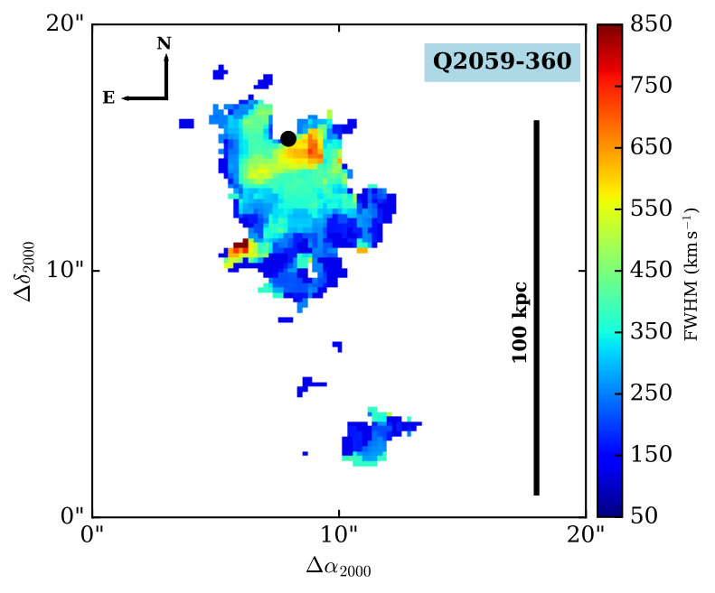 Figure 1
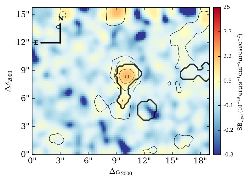 Figure 2
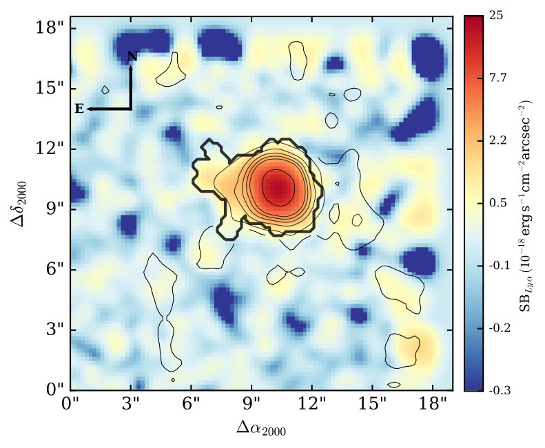 Figure 3
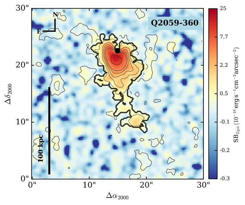 Figure 4
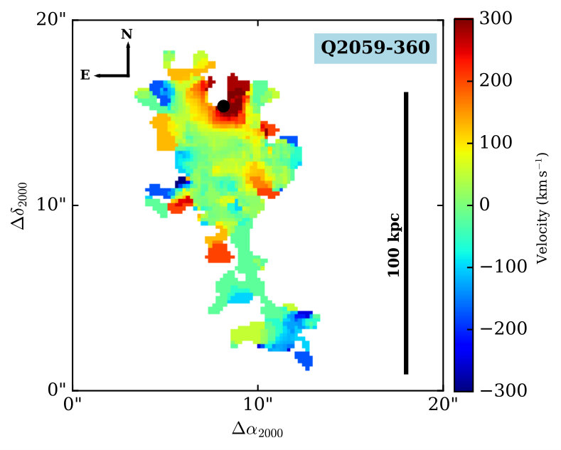 Figure 5
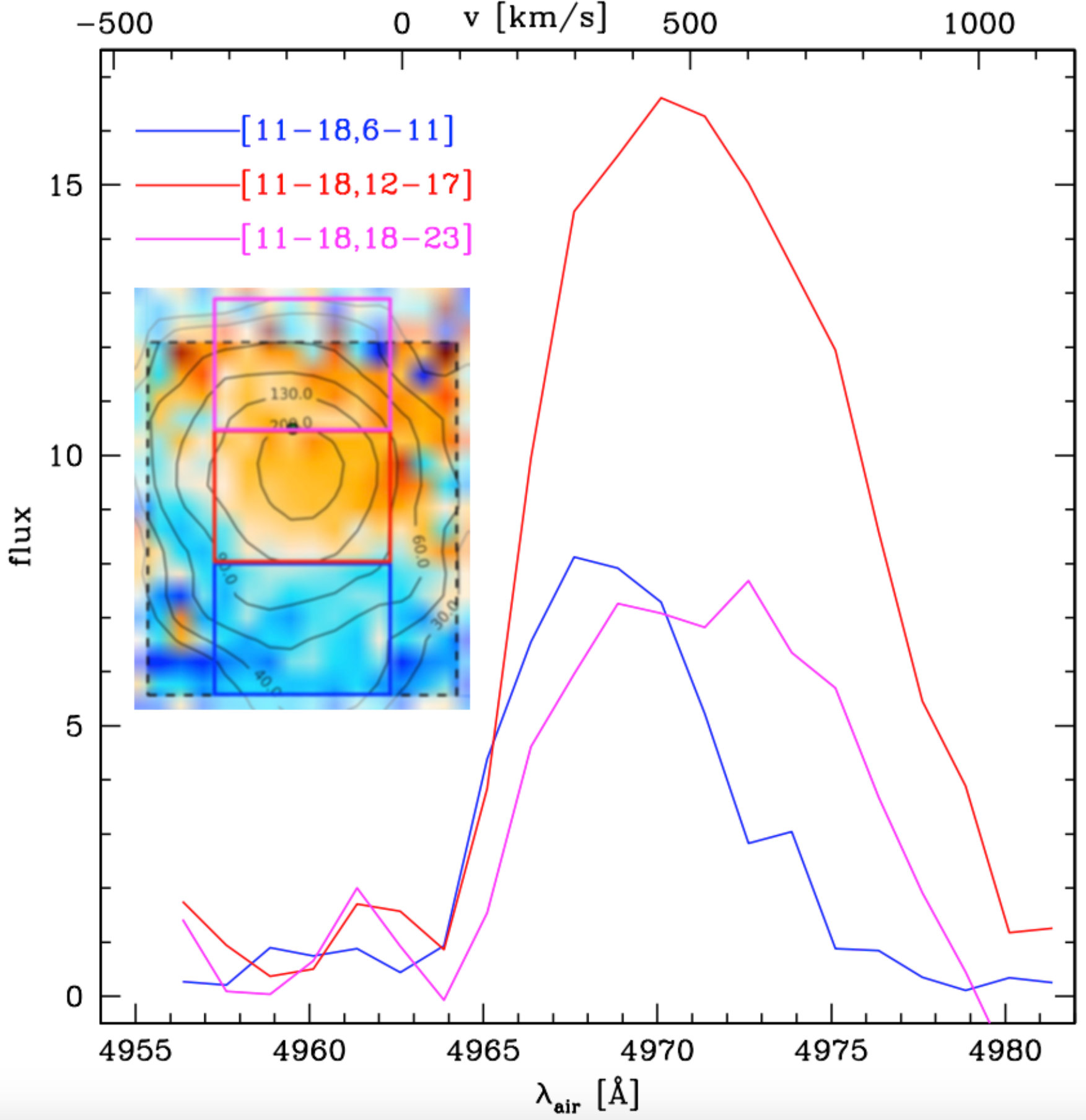 Figure 6
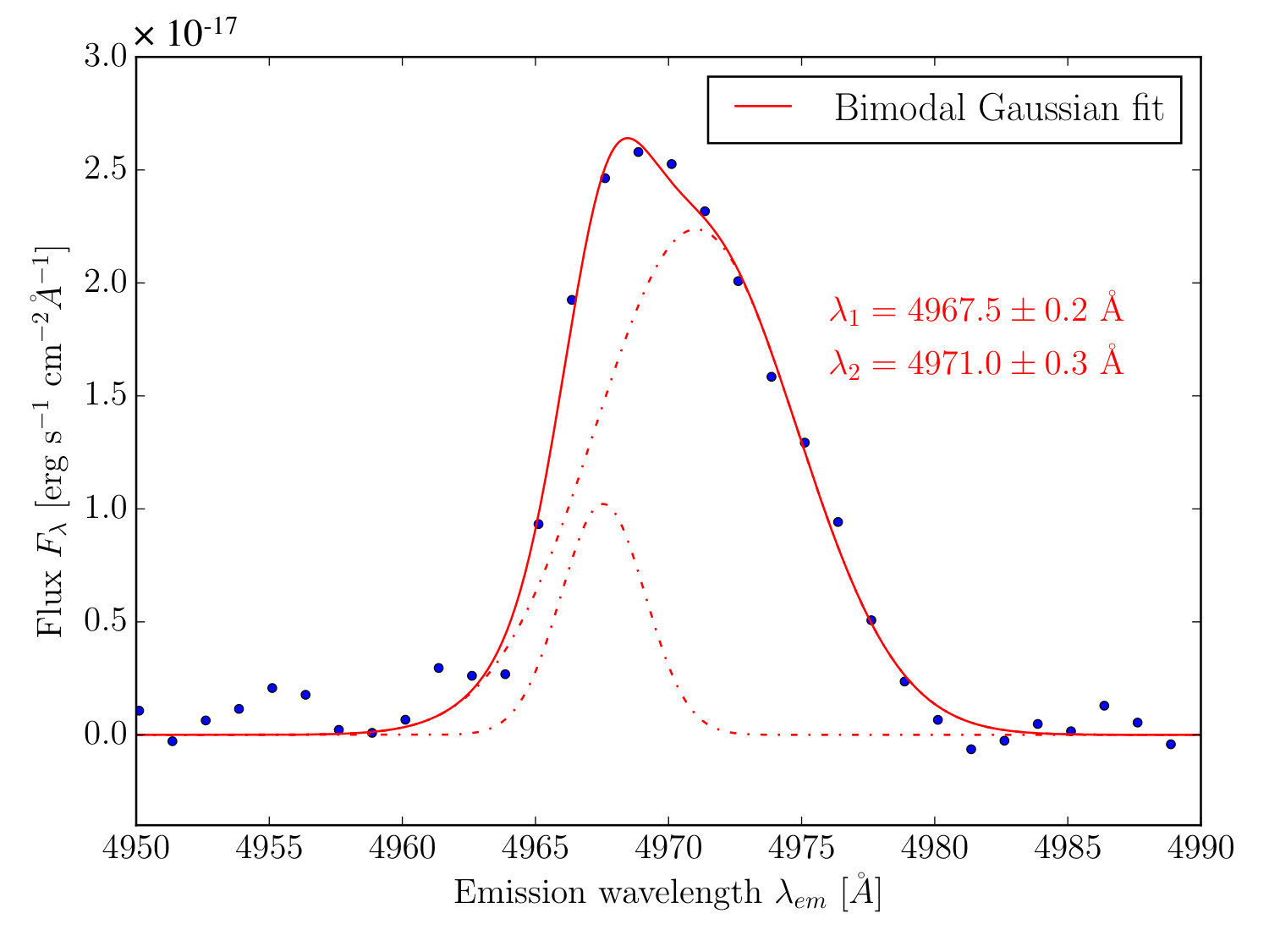 Figure 7
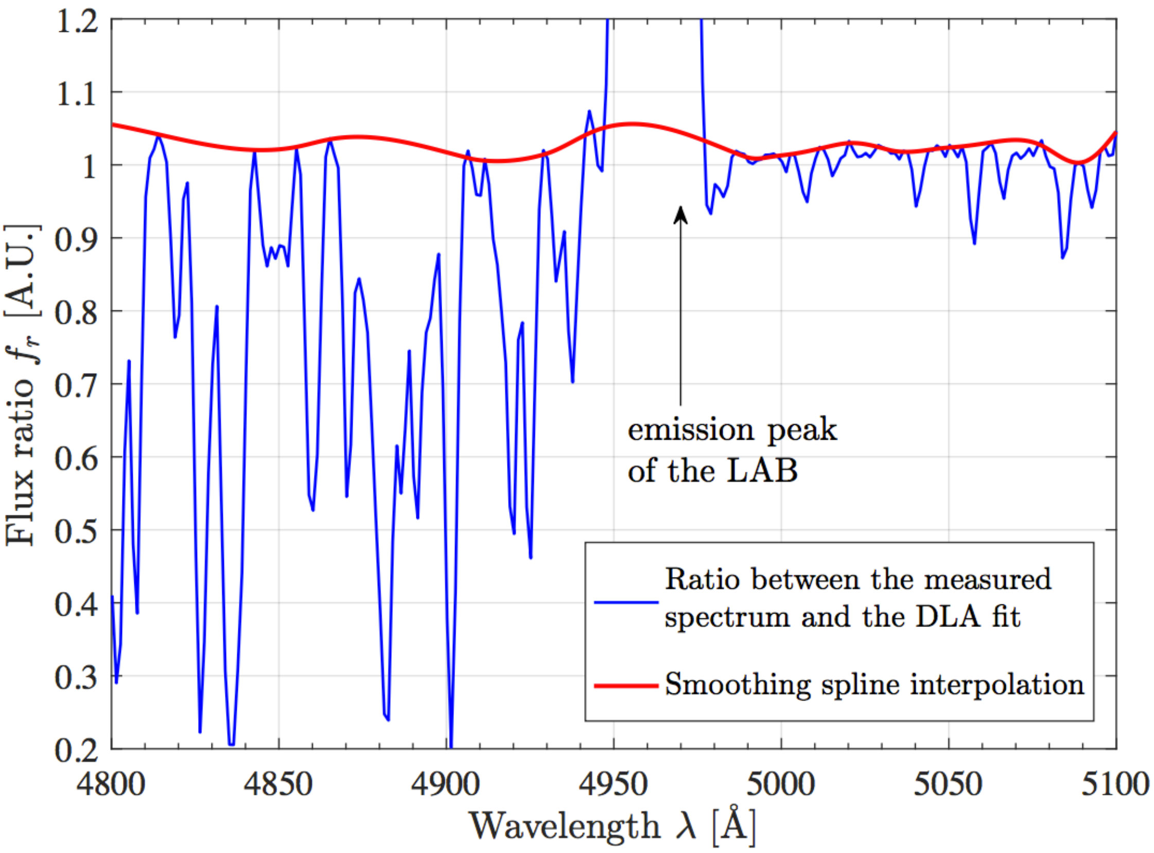 Figure 8
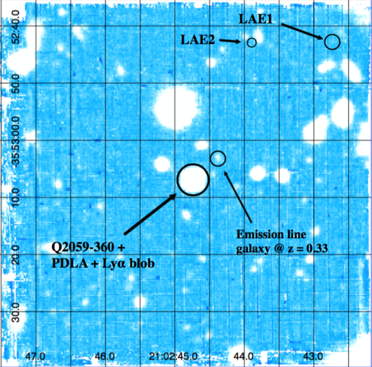 Figure 9
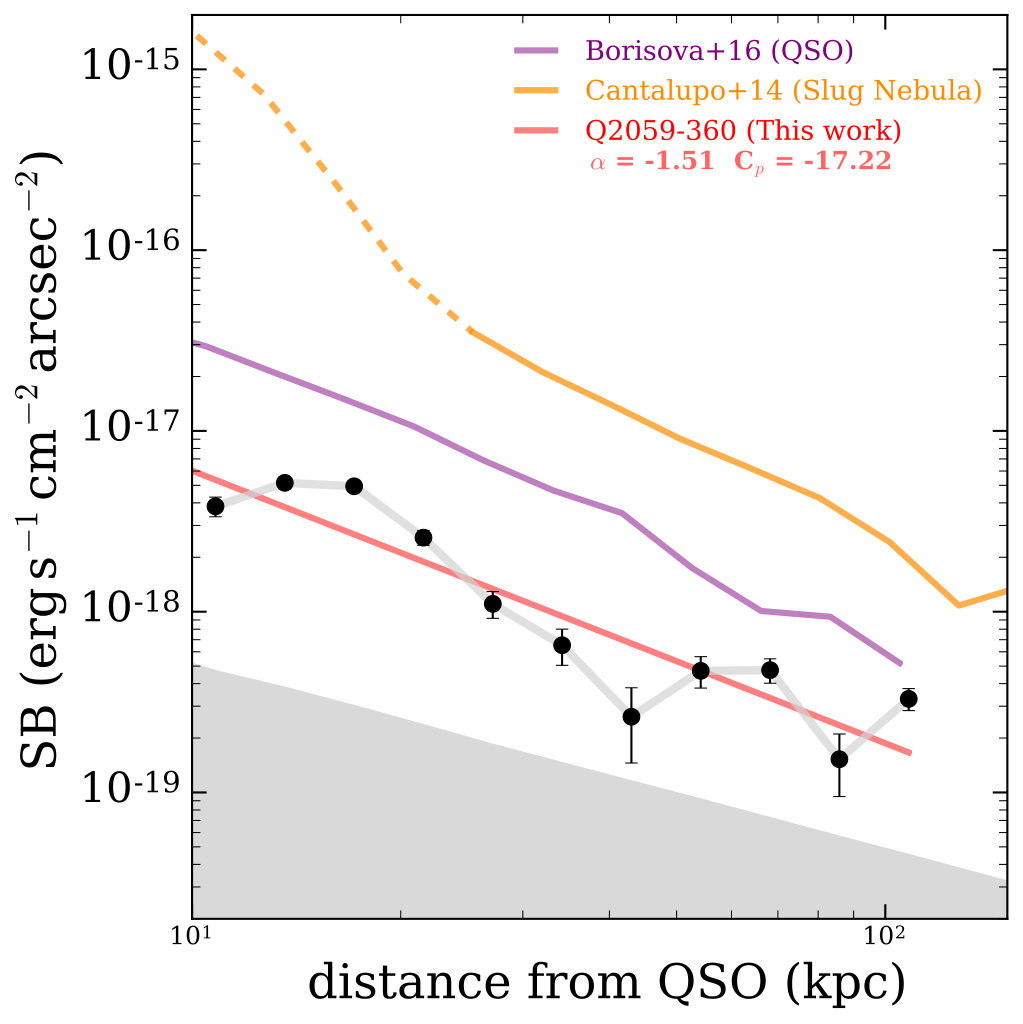 Figure 10
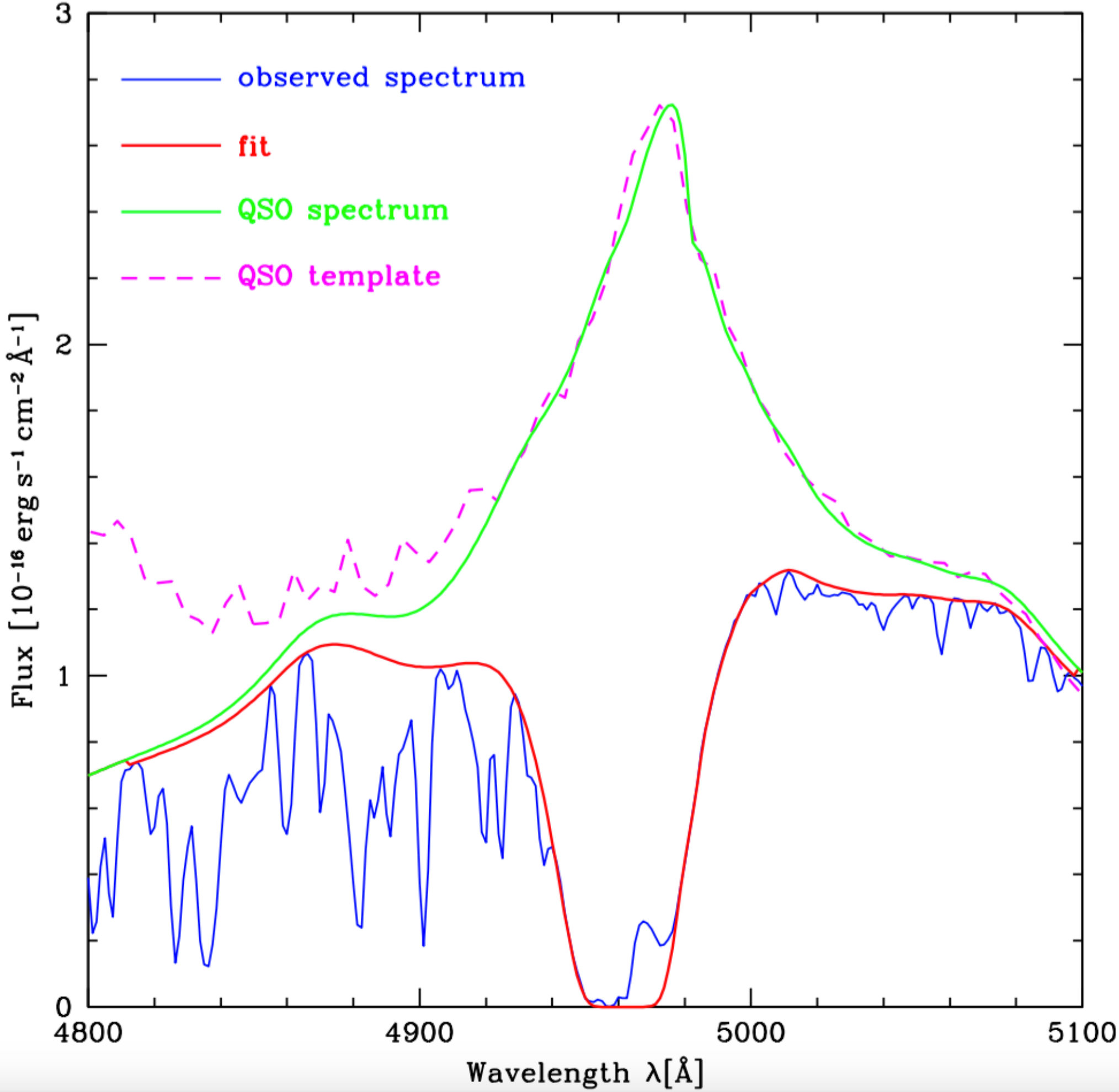 Figure 11
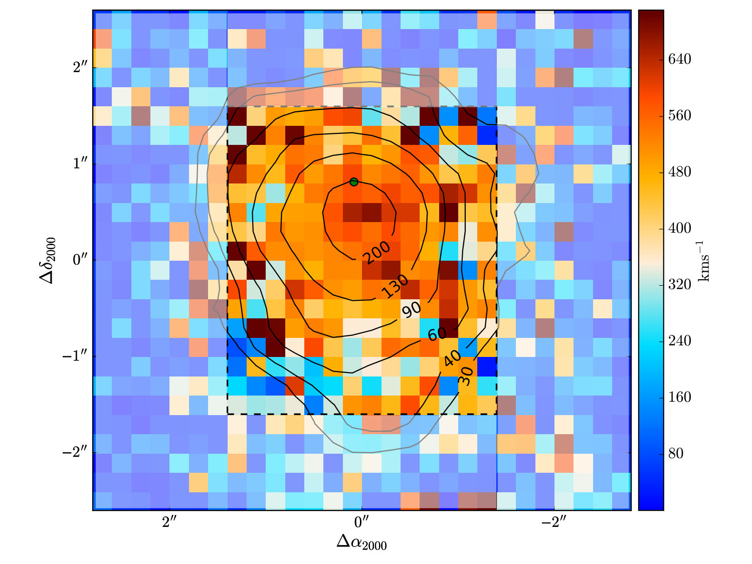 Figure 12
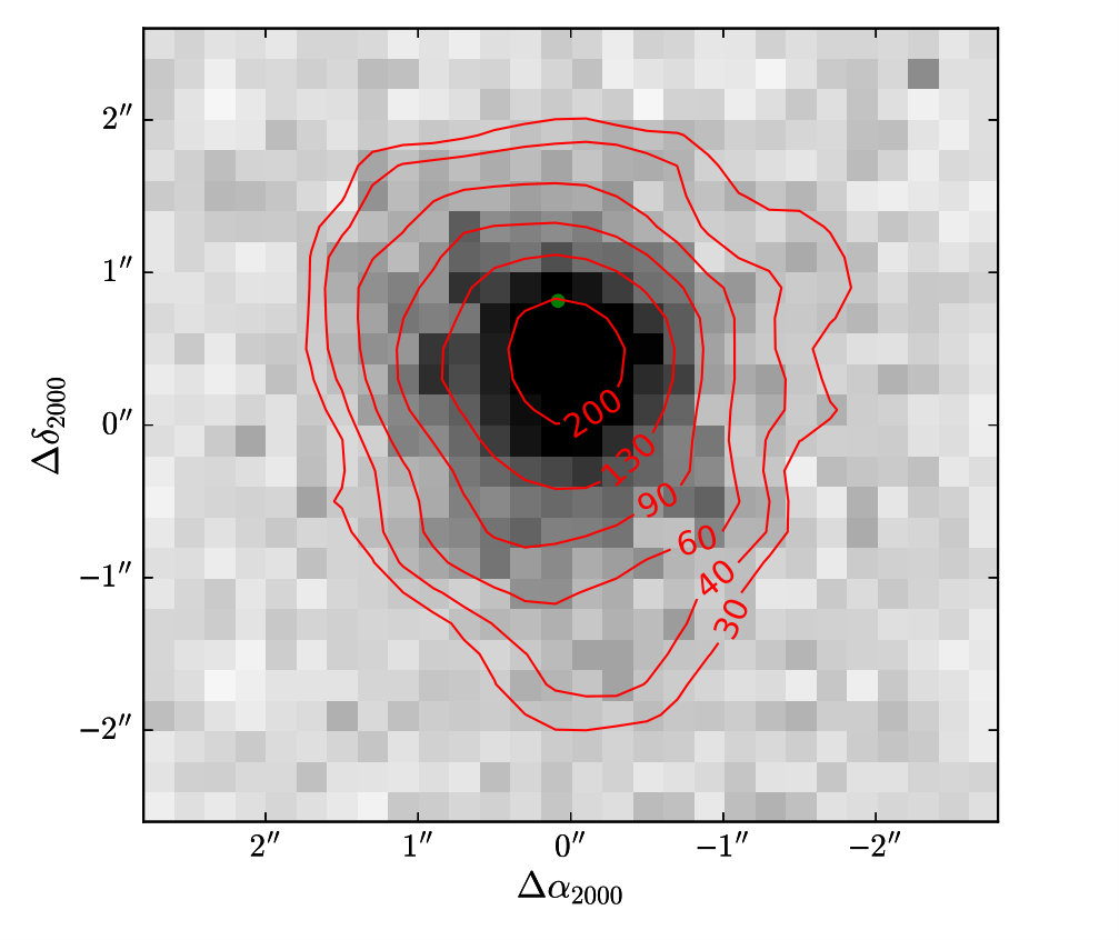 Figure 13
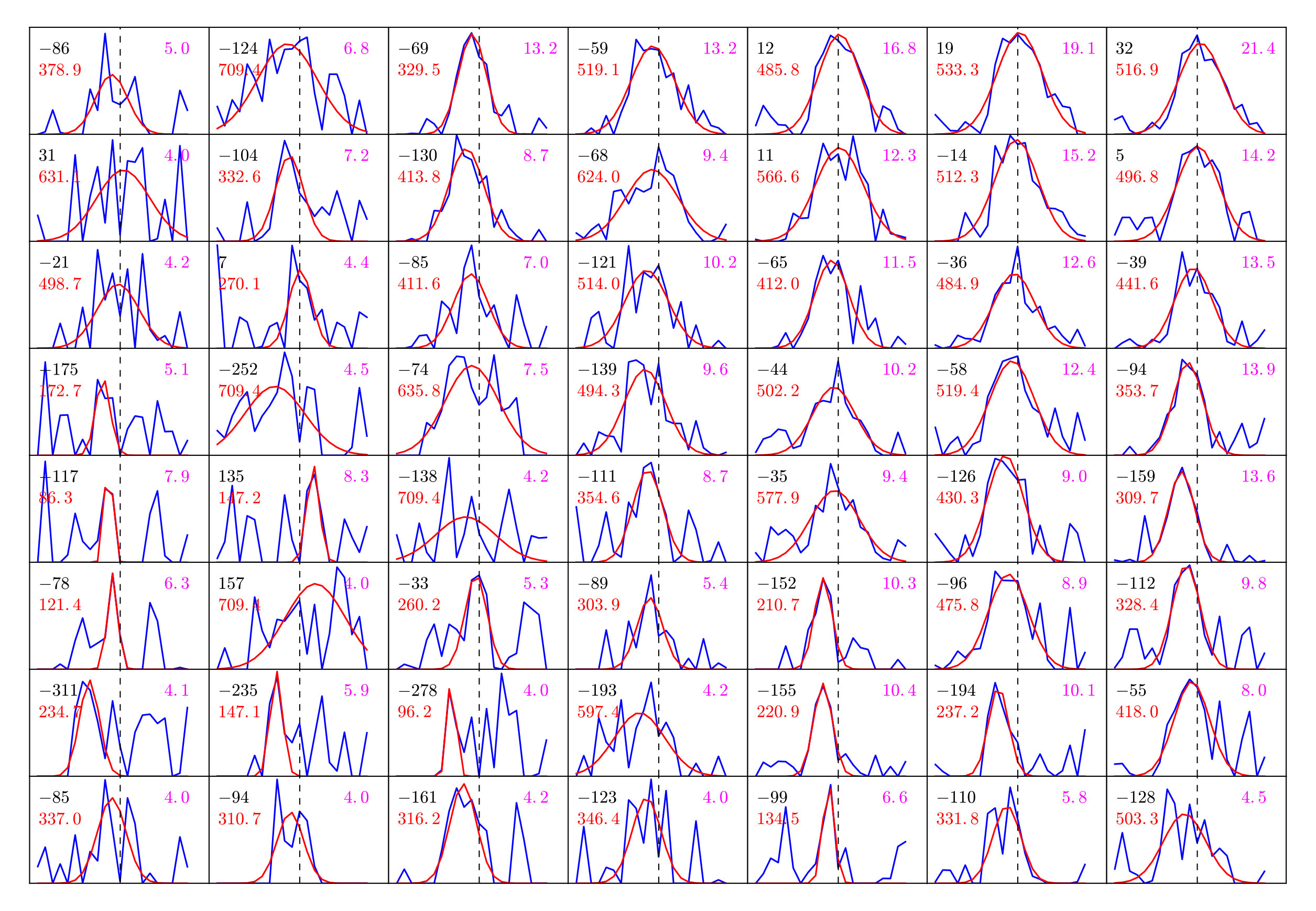 Figure 14
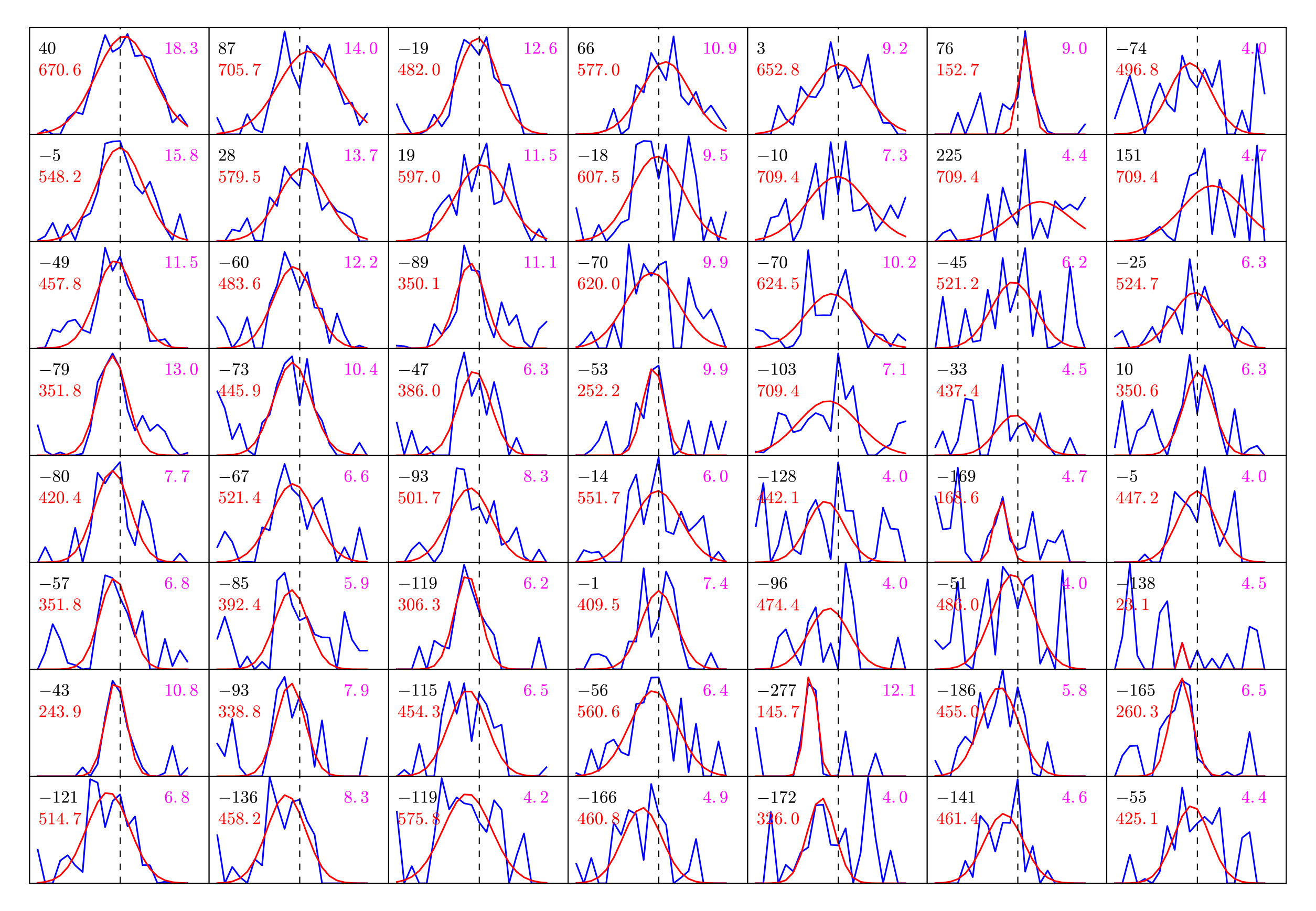 Figure 15
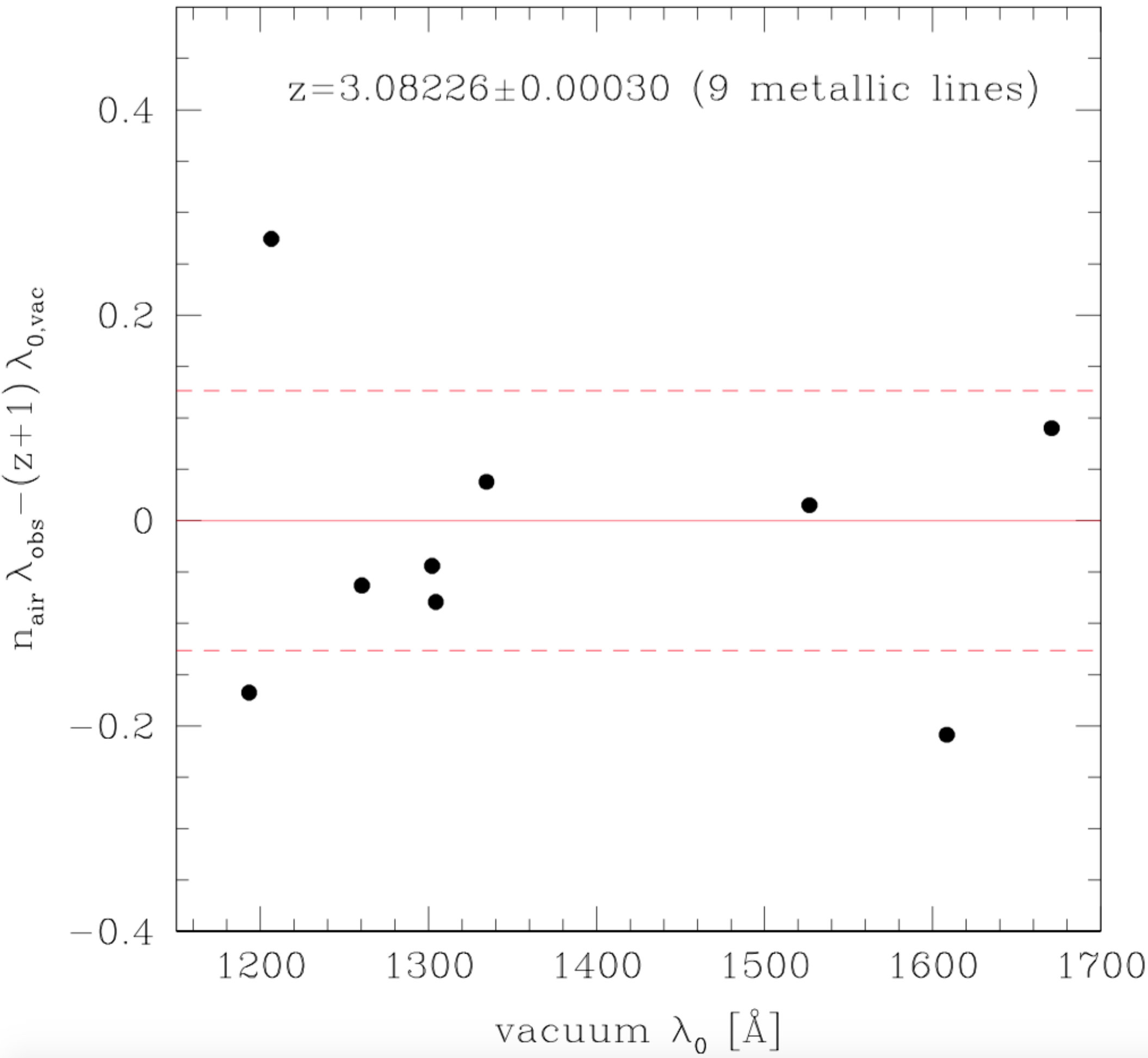 Figure 16
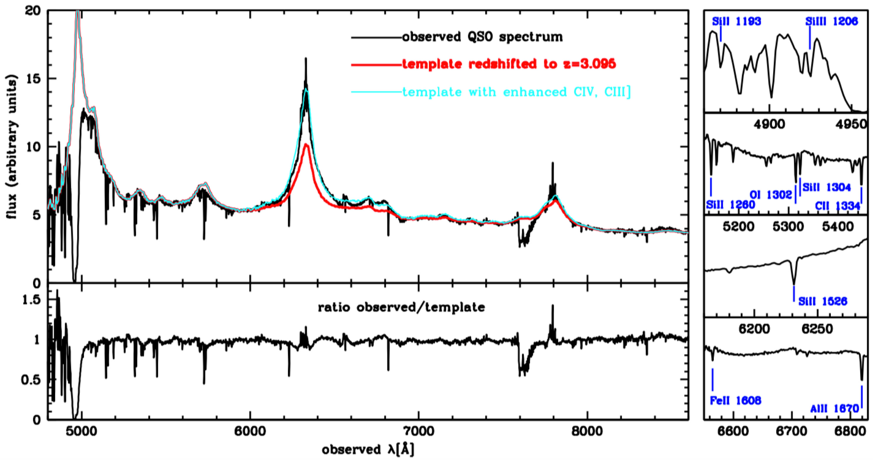 Figure 17
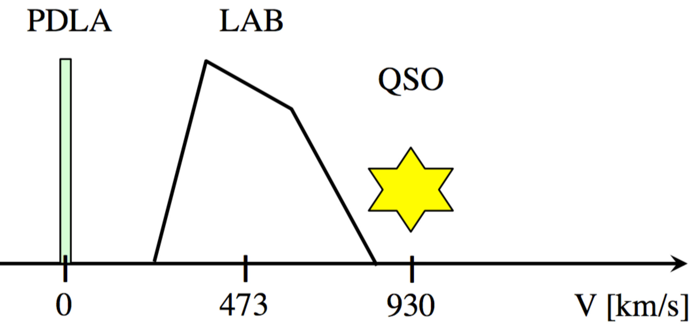 Figure 18
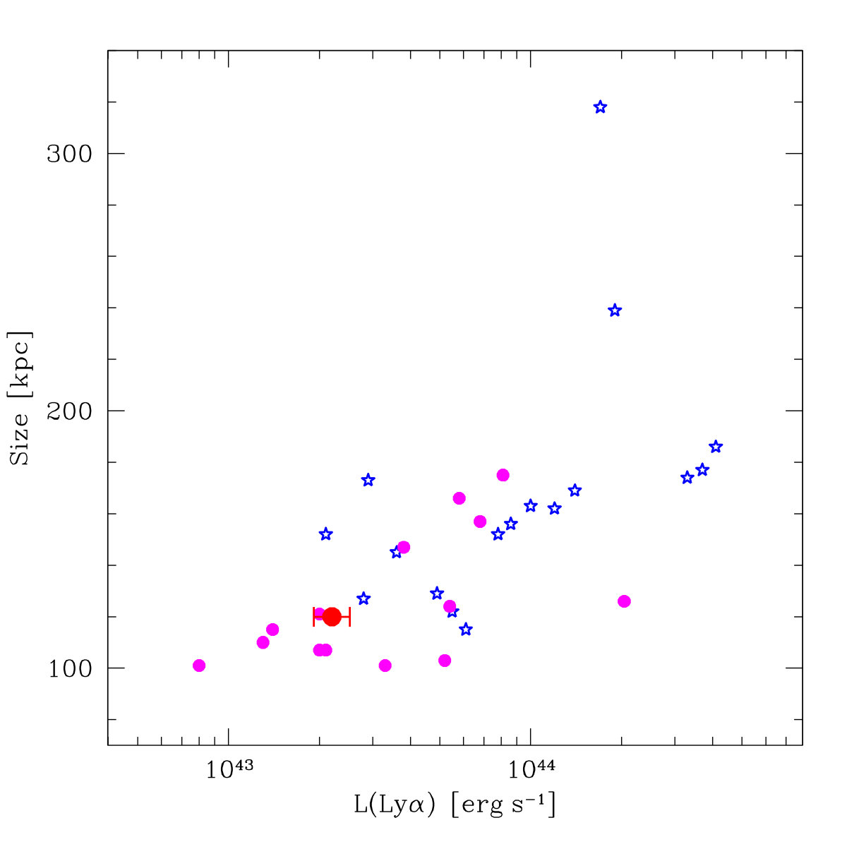 Figure 19
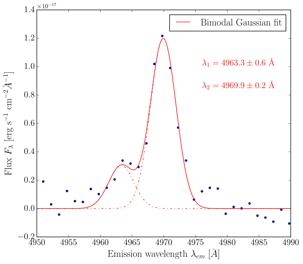 Figure 20
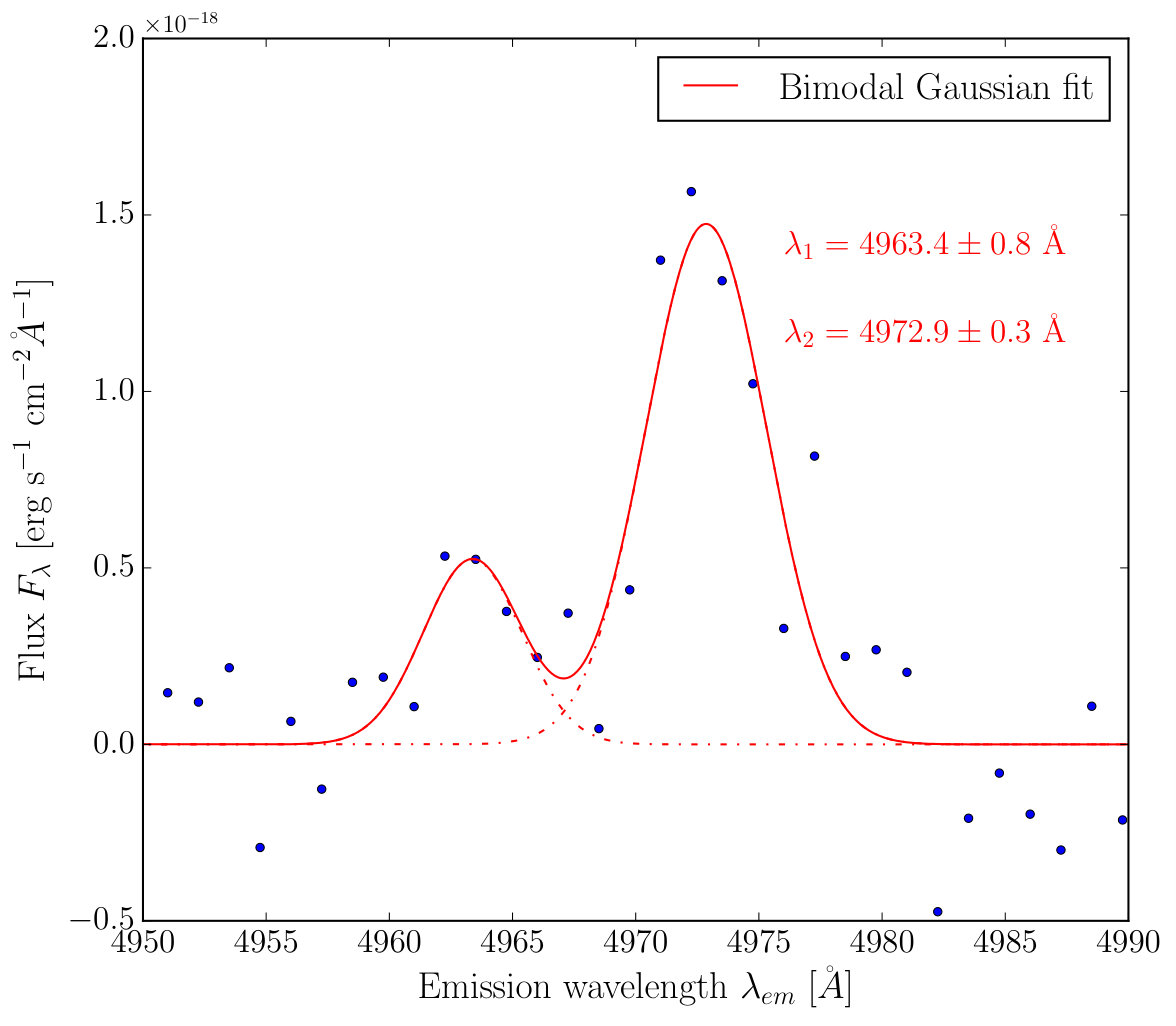 Figure 21
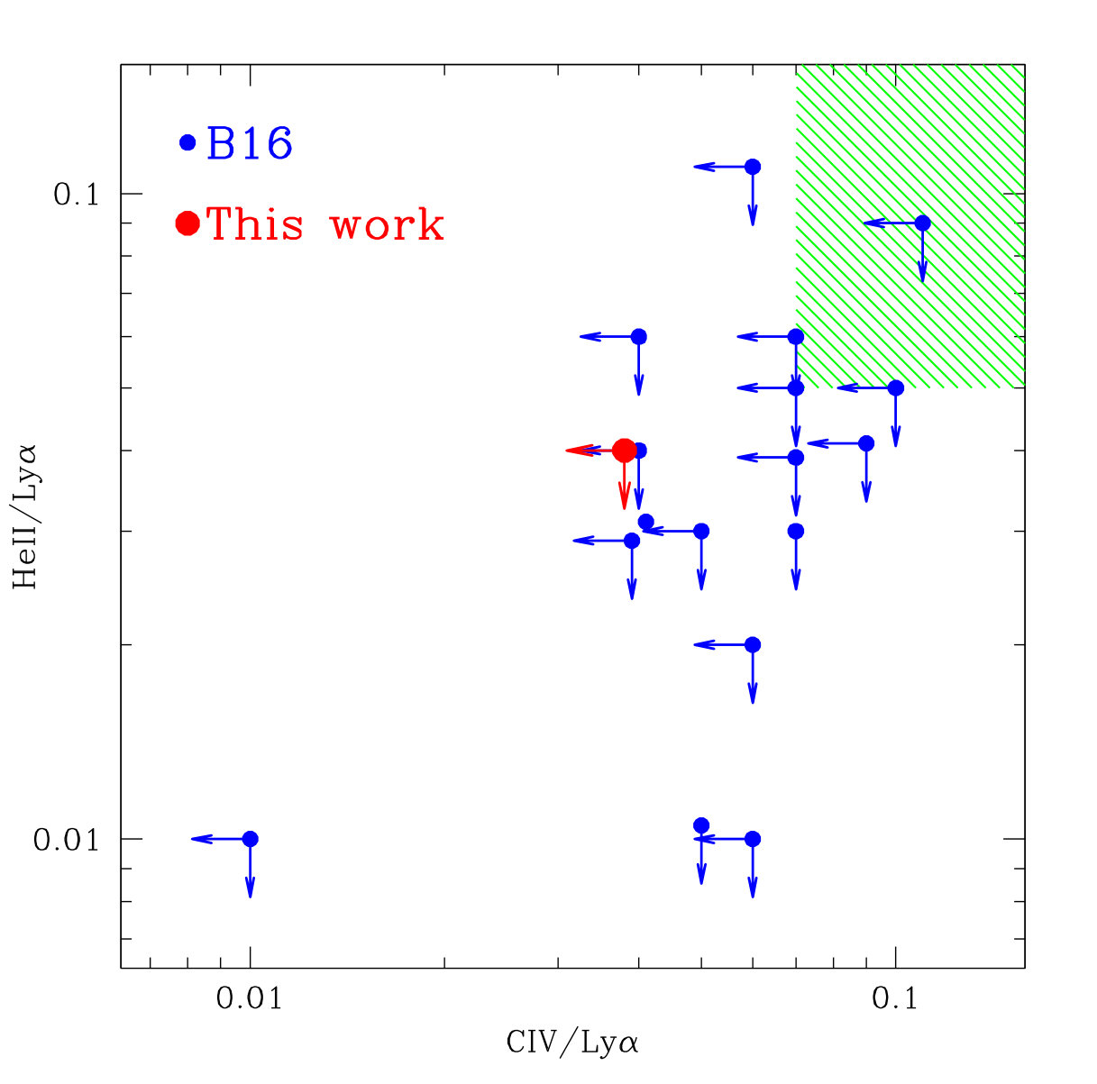 Figure 22
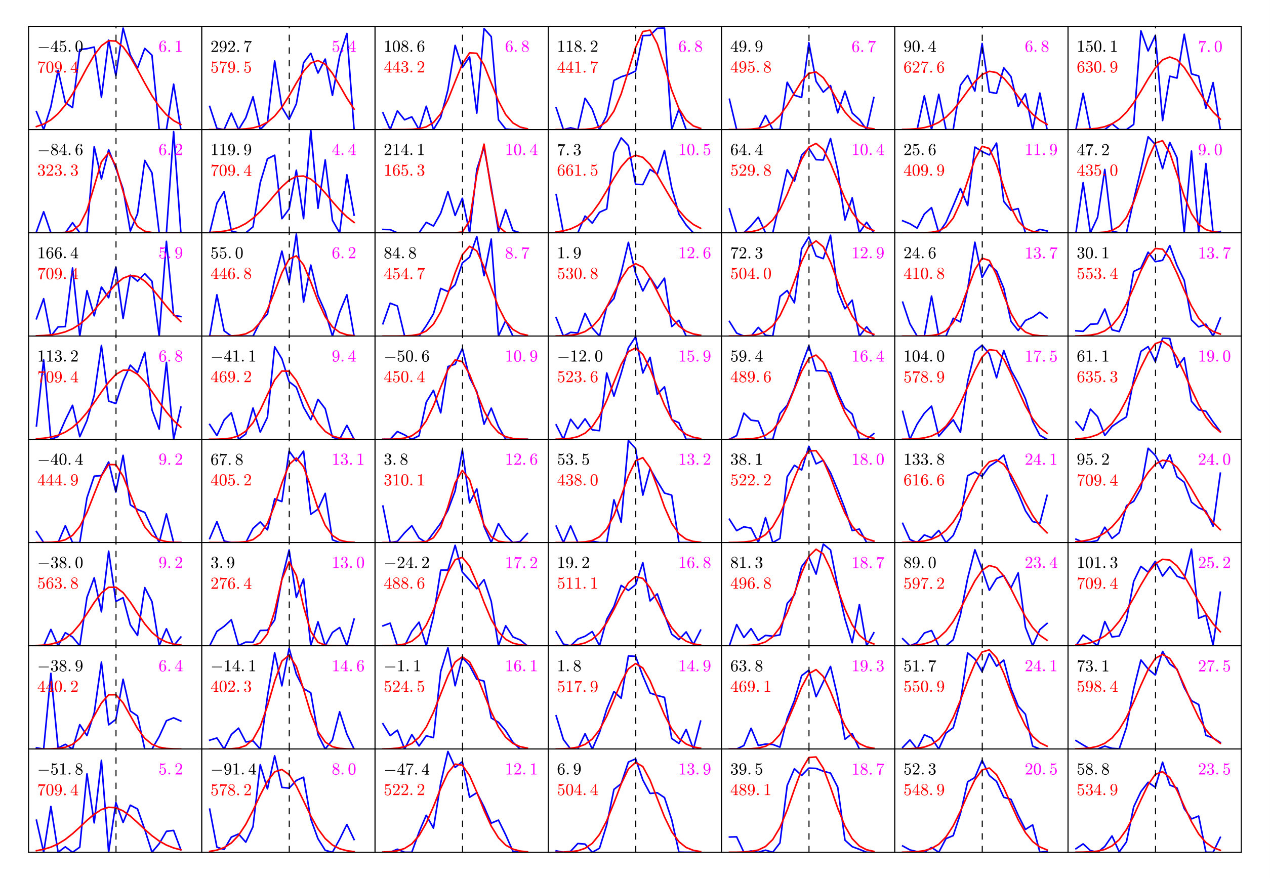 Figure 23
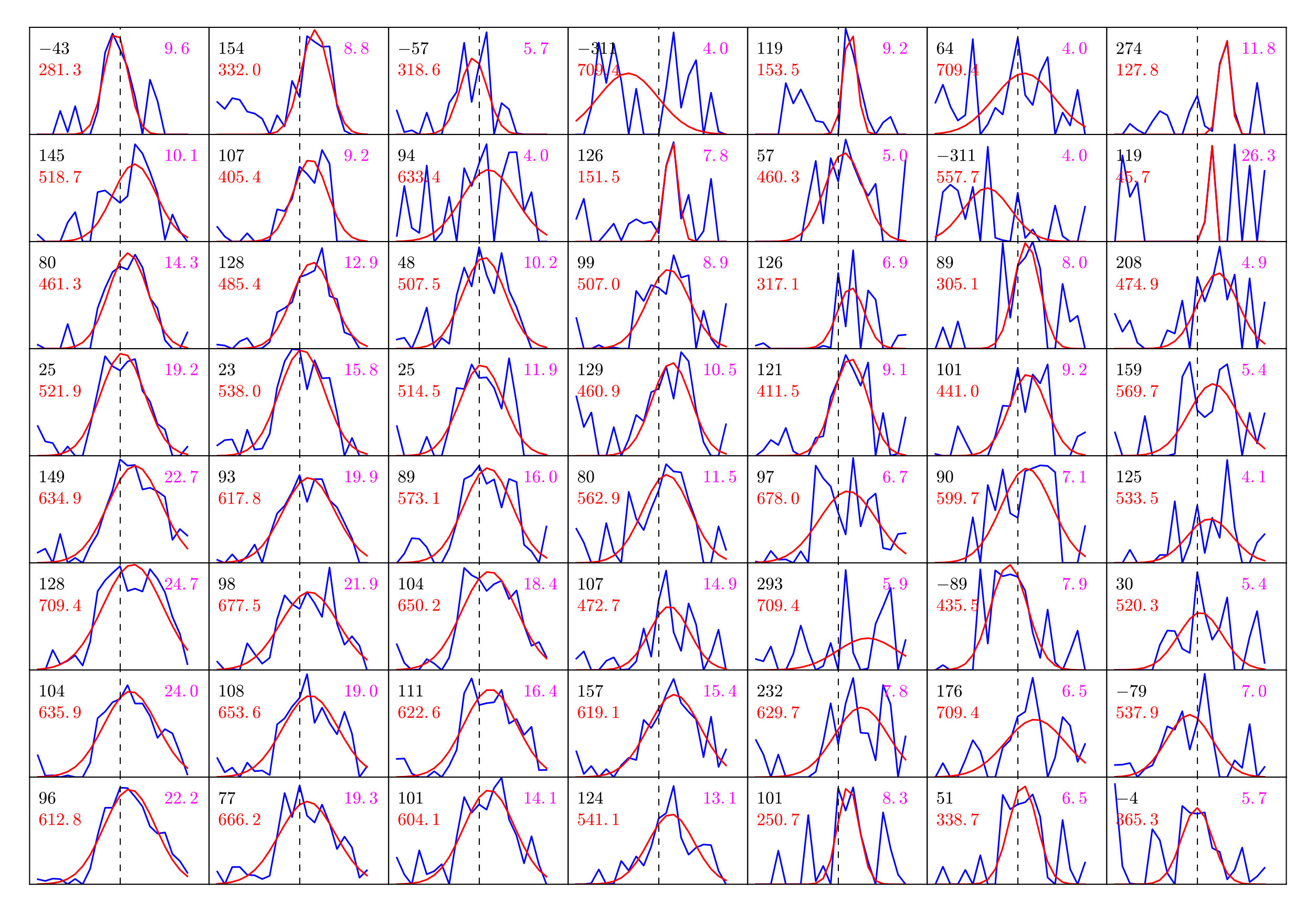 Figure 24
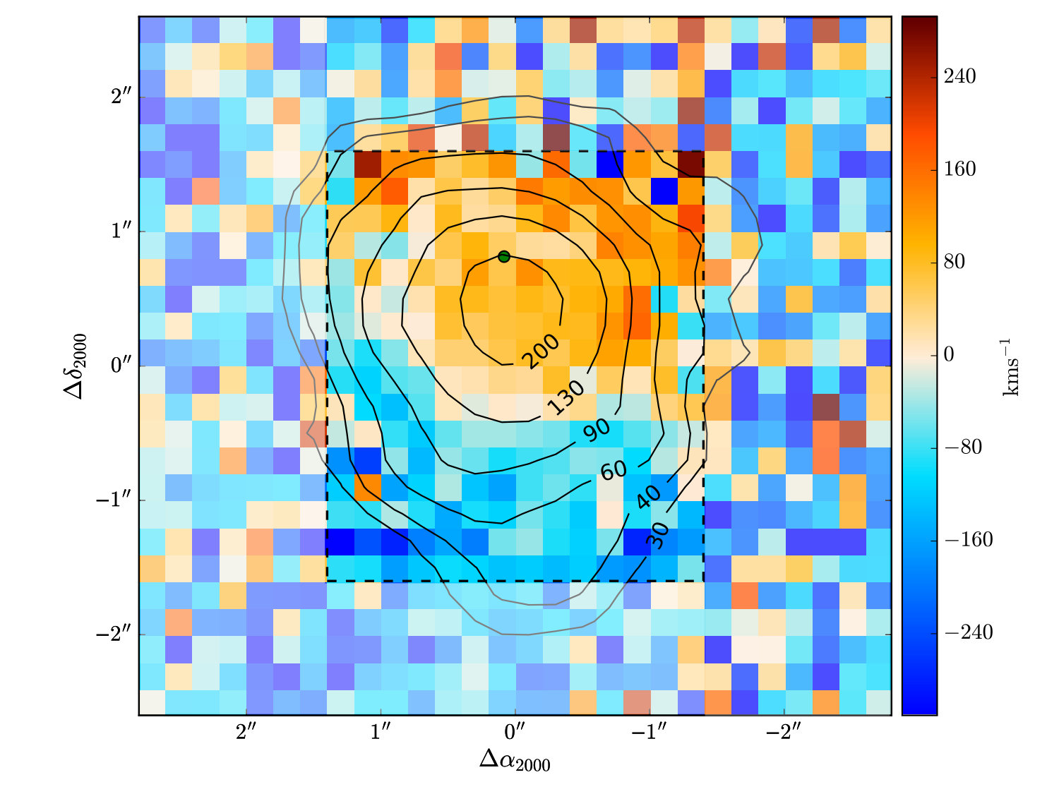 Figure 25
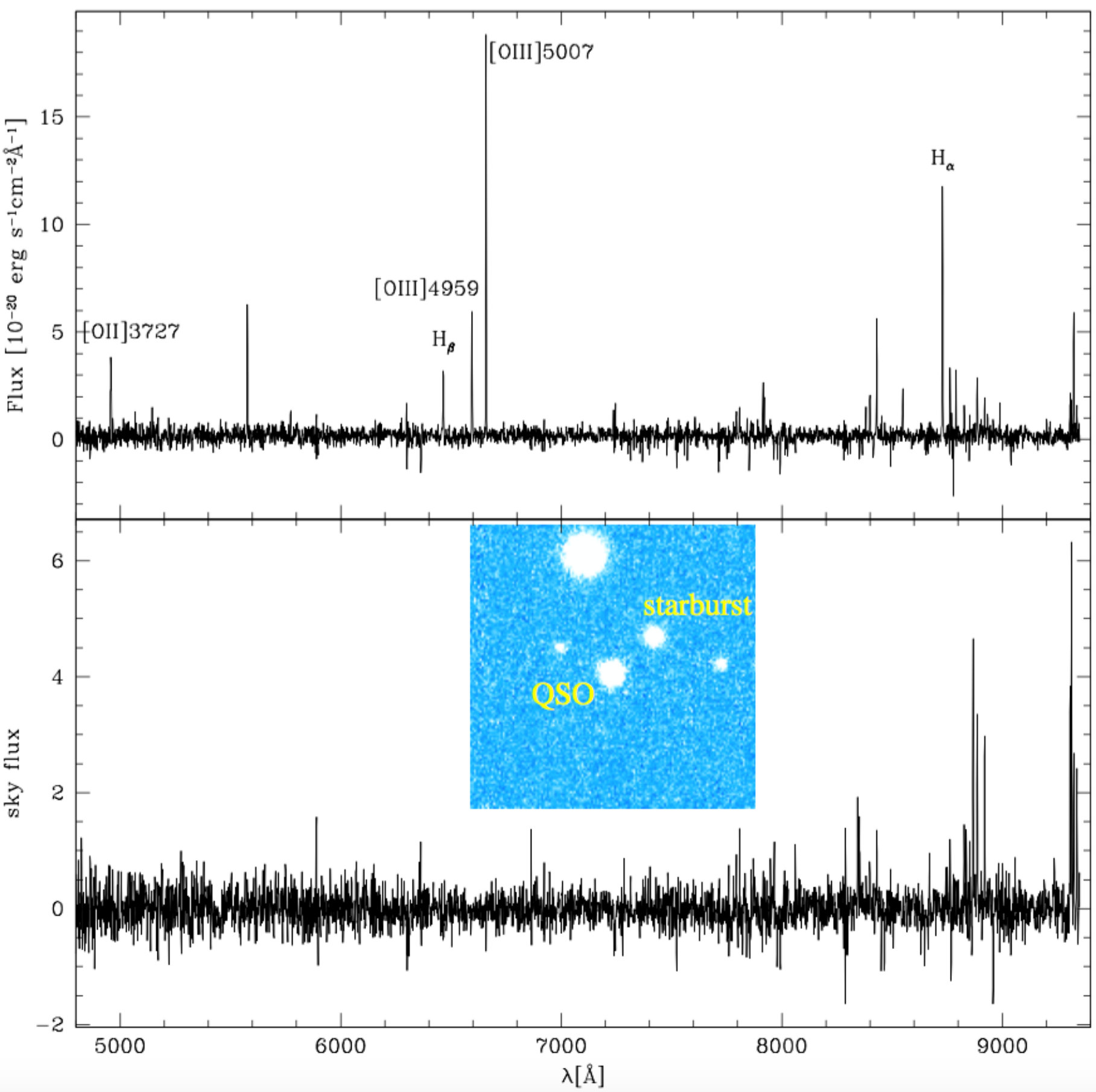 Figure 26
| FWHM | FWHM | ||
|---|---|---|---|
| [Å] | [km s-1] | [Å] | |
| first peak | |||
| second peak | |||
| first moment |
| Line, (vac.) | Flux ( limit) | |
|---|---|---|
| [Å] | [ erg/s/cm2/arcsec2] | |
| N V | ||
| C IV | ||
| He II | ||
| C III] |
| Object | (J2000) | peak | z | FWHM | ||||
|---|---|---|---|---|---|---|---|---|
| [h:m:s] | [°:’:”] | [Å] | [km s-1] | [] | [km s-1] | |||
| LAE1 | blue | |||||||
| red | ||||||||
| LAE2 | blue | |||||||
| red | ||||||||
| [h:mn:s] | [°:′:″] |
|---|---|
| Line | Observed flux [ erg s-1 cm-2] |
| [O II] | |
| Hβ | |
| [O III] | |
| [O III] | |
| Hα | |
| [N II] |
Peer Reviews
No public reviews on file for this paper yet. If you reviewed it on a platform where reviews are public (OpenReview, ICLR, NeurIPS, ICML), you can paste yours below so the community can read it here.
Videos
No videos yet. Explain this paper in a talk, walkthrough, or lecture? Add one.
11institutetext: Institute of Physics, Laboratory of Astrophysics, École Polytechnique Fédérale de Lausanne (EPFL),
Observatoire de Sauverny, 1290 Versoix, Switzerland 22institutetext: Institute for Astronomy, ETH Zürich, Wolfgang-Pauli Strasse 27, 8093 Zürich, Switzerland 33institutetext: Department of Astronomy, Oskar Klein Centre, Stockholm University, AlbaNova University Centre, SE–106 91 Stockholm, Sweden 44institutetext: STAR Institute, Quartier Agora – Allée du six Août 19c, B-4000 Liège, Belgium 55institutetext: Department of Physics, University of Haifa, Mount Carmel, Haifa 31905, Israel 66institutetext: Observatoire de Genève, Université de Genève, Ch. des Maillettes 51, 1290 Versoix, Switzerland
MUSE-inspired view of the quasar Q2059-360, its Lyman blob,
and its neighborhood††thanks: Based on observations collected at the European Organisation for Astronomical Research in the Southern Hemisphere under ESO programme 60.A-9331(A)
P. L. North 11
R. A. Marino 22
C. Gorgoni 11
M. Hayes 33
D. Sluse 44
D. Chelouche 55
A. Verhamme 66
S. Cantalupo 22
F. Courbin 11
(Received / Accepted )
The radio-quiet quasar Q2059-360 at redshift is known to be close to a small Lyman blob (LAB) and to be absorbed by a proximate damped Ly (PDLA) system.
Here, we present the Multi Unit Spectroscopic Explorer (MUSE) integral field spectroscopy follow-up of this quasi-stellar object (QSO). Our primary goal is to characterize this LAB in detail by mapping it both spatially and spectrally using the Ly line, and by looking for high-ionization lines to constrain the emission mechanism.
Combining the high sensitivity of the MUSE integral field spectrograph mounted on the Yepun telescope at ESO-VLT with the natural coronograph provided by the PDLA, we map the LAB down to the QSO position, after robust subtraction of QSO light in the spectral domain.
In addition to confirming earlier results for the small bright component of the LAB, we unveil a faint filamentary emission protruding to the south over about pkpc (physical kpc); this results in a total size of about pkpc. We derive the velocity field of the LAB (assuming no transfer effects) and map the Ly line width. Upper limits are set to the flux of the N v , C iv , He ii , and C iii] lines. We have discovered two probable Ly emitters at the same redshift as the LAB and at projected distances of kpc and kpc from the QSO; their Ly luminosities might well be enhanced by the QSO radiation. We also find an emission line galaxy at near the line of sight to the QSO.
This LAB shares the same general characteristics as the others surrounding radio- quiet QSOs presented previously. However, there are indications that it may be centered on the PDLA galaxy rather than on the QSO.
Key Words.:
quasars: general - quasars: Q2059-360 - quasars: emission lines - galaxies: high redshift - intergalactic medium - cosmology: observations - Lyman blobs (LABs)
1 Introduction
Lyman (Ly) nebulae have been discovered around many quasi-stellar objects (QSOs) and radio-galaxies at high redshift through slit spectroscopy (Heckman et al. 1991; Lehnert & Becker 1998; Bunker et al. 2003; Villar-Martín et al. 2003; Weidiger et al. 2005; van Breugel et al. 2006; Willott et al. 2011; North et al. 2012), narrow-band imaging (Hu & Cowie 1987; Steidel et al. 2000; Smith & Jarvis 2007; Yang et al. 2014), and more recently, through integral field spectroscopy (hereafter IFS) (Christensen et al. 2006; Francis & McDonnell 2006; Herenz et al. 2015; Borisova et al. 2016). They easily span tens of physical kiloparsecs (pkpc) and may be larger than pkpc. Those that host a radio galaxy or a radio-loud QSO are brighter than those hosting a radio-quiet QSO (RQQ), presumably because in the former, interactions between the relativistic jet and the circum-galactic gas enhances ionization (Villar-Martín et al. 2003). The Ly nebulae surrounding an RQQ or that host no remarkable object are also called Ly blobs (LABs). Although they do not necessarily host a QSO or active galactic nucleus (AGN), they are found preferentially in overdense regions (Erb et al. 2011; Matsuda et al. 2004, 2009, 2011; Prescott et al. 2008; Yang et al. 2009). These nebulae are interesting because they trace the circum-galactic medium (CGM) at high redshifts, thereby probing galaxy formation, especially if their Ly fluorescence is enhanced by the ultraviolet (UV) radiation of the QSO, as outlined by Haiman & Rees (2001) and Cantalupo et al. (2005, 2007, 2012).
Although most LABs remain confined within the virial radii of their respective haloes, recent observations have uncovered remarkably large nebulae extending beyond the virial radius (Cantalupo et al. 2014; Martin et al. 2014a, b, 2015; Hennawi et al. 2015), with typical sizes of pkpc. These outstanding observations, some of them made possible by new-generation IFSs like the Palomar Cosmic Web Imager (Martin et al. 2014a, b, 2015), provide the first evidence of the cosmic web filaments predicted by large-scale CDM simulations.
The frequency of LABs around RQQs has remained an open question (e.g., North et al. 2012) until the new-generation IFS Multi Unit Spectroscopic Explorer (MUSE) attached to the fourth unit of the VLT at ESO was used to observe 17 RQQs at redshifts and found an LAB around each of them (Borisova et al. 2016, hereafter B16). Therefore, in this redshift range and for a sensitivity of about erg s*-1* cm*-2* arcsec*-2*, the frequency of LABs surrounding RQQs is %. Moreover, the size of such nebulae always reaches or exceeds pkpc, and their surface brightness (SB) profiles are consistent with a power law with a slope of about .
Obviously, the ubiquity and similarity of the LABs that enshroud RQQs raise the question of their power source and emission mechanism. In addition to fluorescent emission from photo-excitation or photoionization (e.g., Geach et al. 2009), other power sources have been suggested, like cooling radiation where gravitational energy of the gas collapsing in the potential well of the dark matter halo is converted into Ly radiation after collisional excitation and ionization (known also as the “cold accretion” scenario, see, e.g., Haiman et al. 2000; Fardal et al. 2001; Dijkstra & Loeb 2009; Rosdahl & Blaizot 2012). Shock heating was also proposed (Taniguchi & Shioya 2000; Mori et al. 2004). Finally, scattering of the Ly photons emitted by a central source (like an AGN) may also occur, betrayed by a high level of linear polarization in the external parts of the nebula (Lee & Ahn 1998; Rybicki & Loeb 1999; Dijkstra & Loeb 2008, 2009; Dijkstra & Kramer 2012). This effect was first observed by Hayes et al. (2011) and may coexist with the cold accretion scenario (Trebitsch et al. 2016). Additional lines such as He ii can potentially help distinguish between the cold accretion and the photoionization scenarios, although very deep obervations seem to be needed (Arrigoni Battaia et al. 2015).
Neutral hydrogen clouds may lie on the line of sight of a QSO and produce a so-called damped Lyman alpha (DLA) absorption system, as soon as the column number density exceeds cm*-2*. When the velocity difference between the DLA and the background QSO is km s*-1*, the two objects are considered as being “associated” and the DLA is then classified as a proximate damped Lyman alpha (PDLA) system (Ellison et al. 2002, 2010). Even though the association may not be physical in the gravitational sense, it can be manifested through enhanced incidence of highly ionized species, for example, showing that the absorber is “influenced by the radiation field of the QSO”, as Richards (2001) phrased it. The frequency of PDLAs is close to % of the QSOs observed in the redshift range , and at redshift , it exceeds the frequency expected assuming that they are drawn from the same population as the intervening DLAs (Prochaska et al. 2008; Ellison et al. 2010). In addition to its intrinsic interest, a PDLA provides the advantage of acting like a natural coronagraph that extincts the QSO light in the vicinity of the Ly line, allowing us to detect and study any emission nebula surrounding the QSO more easily (Hennawi et al. 2009). This configuration, where the PDLA lies in front of the QSO and its Ly nebula, in principle offers the possibility to “image the PDLA in silhouette against the extended screen of Ly emission”, as outlined by Hennawi et al. (2009).
In this work we focus on an LAB lying along the line of sight of the QSO Q2059-360 (RA 21 02 44, Dec -35∘ 53*′* 06.5*′′, V) at redshift (Warren et al. 1991)111This is the original reference. The redshift value is mentioned as uncertain for this particular object, while the average error of most other objects is announced to be better than . The LAB is emitting at Å, within the damped Ly absorption (DLA) trough of the QSO spectrum. The DLA that we analyze in this work is at redshift , that is, only km s-1* from the background QSO, if the latter is indeed at redshift ; our revised redshift estimate is rather (see Sects. 3.1 and 3.3 below), implying a velocity difference of km s*-1* (see Sect. 3.2 below). This would represent proper Mpc if the velocity difference were entirely due to the Hubble flow222http://home.fnal.gov/~gnedin/cc/. An early study of this QSO and of its Ly features has been carried out by Leibundgut & Robertson (1999). Based on long-slit spectra, they showed that the emission feature is extended both spatially and spectrally, and they provided evidence for a shift of the central wavelength as a function of the offset position from the QSO. Here, we take advantage of the IFS to provide a detailed 2D mapping of the structure.
In our analysis, we assume a CDM universe model with parameters km s*-1Mpc-1*, , and (Bennett et al. 2014), and we use the cosmology calculator made available by Wright (2006) on the World Wide Web333http://www.astro.ucla.edu/~wright/CosmoCalc.html.
2 Observations and data reduction
The MUSE instrument is an IFS located at the Nasmyth B focus of Yepun, the VLT UT4 telescope. It is operating in the visible wavelength range from 4800 Å to 9400 Å. Thanks to its wide field of view, in the wide field mode, it is able to take simultaneous spectra with a spatial sampling of ″per pixel (also referred to as ”spaxel”). MUSE has a resolving power (Richard & Bacon 2014) at the redshifted Ly wavelength, which in terms of velocity separation corresponds to a resolution of
[TABLE]
where is the speed of light in the air. Or equivalently in terms of wavelength,
[TABLE]
where Å is the wavelength of the Ly blob emission at redshift .
The observations were made in June 2014 during the science verification phase (ESO program 60.A-9331(A)). The total exposure time amounts to 3 hours 20 minutes, distributed in four observing blocks, each of which included two s exposures taken at instrumental position angles differing by . Dithering of a few arcseconds was also applied.
The data set was reduced using both the ESO MUSE pipeline (version 1.6, Weilbacher 2015) and the CubExtractor package (CubEx hereafter, version 1.6; Cantalupo, in preparation). In particular, the basic reduction steps of bias and flat-fielding corrections, wavelength solution, illumination correction, and flux calibration were made for each of the individual exposures with the ESO pipeline using the default parameters. After the calibration files were processed, the raw science data were then reduced using the scibasic and scipost recipes in order to obtain the datacubes and pixel tables for each exposure sampled in a common grid of Å. Then, we made use of the CubEx package to compute a more accurate astrometry, to improve the quality of the flat-field correction (CubeFix tool), and to perform a flux-conserving sky subtraction on the individual flatfield-corrected cubes (CubeSharp). We refer to B16 for a detailed description of the CubEx package. Finally, the eight individual exposures were combined into a final cube using a clipping and mean statistics. The resulting point-spread function (PSF) measured at Å on the final combined cube has a full-width at half-maximum (FWHM) of ″. At the wavelength of the emitter ( Å), it is ″.
The white-light image obtained by collapsing the datacube along the wavelength axis from Å to Å is shown in Fig. 1. The position of the QSO is indicated, as well as that of the LAEs found at same redshift, and of an emission line galaxy at . We examine these four objects in turn below.
3 Analysis of the datacube in the QSO vicinity
First of all, we have redetermined the redshift of the QSO (Sect. 3.1), and the redhift of the PDLA using metallic absorption lines (Sect. 3.2). Then, we have performed two independent analyses of the immediate neighborhood of the QSO, aimed first at characterizing the LAB. The analysis is complicated by the velocity offset between the PDLA absorption trough and the nebular emission, causing the latter to fall not in the middle of the former, but on its red wing. Thus, the QSO contribution has to be subtracted, even though it remains relatively small, at least in its immediate vicinity, namely within ″″ of it. We used the method proposed by Leibundgut & Robertson (1999), which consists of defining the QSO intrinsic spectrum and subtract it in the wavelength domain for each spaxel; for the sake of consistency, we also performed an analysis similar to that presented by B16 (subtraction of the QSO PSF in the spatial plane for each relevant wavelength bin). We describe these two methods in more detail below (Sects. 3.3 and 4.1).
3.1 Redshift of the QSO
We compared the QSO spectrum extracted from the MUSE datacube with the template QSO spectrum built by Vanden Berk et al. (2001) on the basis of SDSS spectra. The latter have about the same resolution as MUSE, making them appropriate for the task. The most useful emission line for redshift determination is C iv, although other features such as Si iv/O iv] and C iii]/Fe iii can also help. After enhancing the line amplitude with respect to the continuum in the template spectrum (by a factor of for C iv and 1.2 for C iii]), the best visual match is obtained for
[TABLE]
as shown in Fig. 2
This is slightly larger than estimated by Warren et al. (1991), but within their error bar. Our redshift estimate is largely based on the C iv line, which is blueshifted on average by km s*-1* with respect to the systemic velocity for radio-quiet quasars (Richards et al. 2011); however, this should also be the case of the template spectrum, so this is not likely to cause any severe bias.
3.2 Redshift of the PDLA according to metallic absorption lines
Ten metallic absorption lines can be easily identified in the PDLA system within the MUSE spectral range. These are Si ii , Si iii , N v , Si ii , O i , Si ii , C ii , Si ii , Fe ii , and Al ii . The N v line is the faintest of all and has the largest residual from the regression of observed versus laboratory wavelengths, so we discarded it. We also discarded the C iv lines because they fall in the middle of telluric lines. The difference between the observed wavelength corrected for the air refraction index () and the redshifted vacuum wavelength is shown in Fig. 3. A least-squares fit weighted by the observed equivalent widths (EW) of the nine lines gives a redshift
[TABLE]
with an rms scatter of Å, much smaller than the spectral resolution. Our estimate agrees with the value of given by Leibundgut & Robertson (1999) (based on the Fe ii , Si ii , and Si iii lines) to within .
There is no sign of any multiple absorption components.
The redshift difference of the PDLA relative to the QSO can be translated into a velocity difference using the formulae given by Davis & Scrimgeour (2014): An object with a “peculiar” redshift with respect to a QSO at redshift will appear to the observer to have such that
[TABLE]
The peculiar velocity is linked to in the following way for relativistic and non-relativistic velocities, respectively:
[TABLE]
where the error reflects the uncertainty on the QSO redshift. Thus we have km s*-1*, justifying the classification of the absorption system as a PDLA.
3.3 Fit of the Lyman alpha absorption trough and subtraction of the QSO contribution
From the whole datacube given by the pipeline, we wish to extract the spectrum of the LAB alone in the vicinity of the QSO. The goal is then to subtract the absorption profile from the observed spectrum to obtain a clear signal of the emission feature without the contribution of the QSO. We first used the ds9 tool to determine the position of the LAB and roughly estimate its extent. This allowed us to select a region encompassing most of the LAB luminosity, and of course the whole QSO contribution. The region we selected is elliptical, with semi-axes of ″ and ″, the position angle (orientation with respect to the north direction, counted positively to the east) of the semi-major axis being °. The procedure to isolate the spectrum of the LAB is then the following:
We use the software VPFit (Carswell & Webb 2014) to fit a Voigt profile to the absorption trough. The needed error vector was extracted from the variance datacube, and we dropped all irrelevant data, namely () absorption lines of the Ly forest, on the blue side of the DLA trough, () some faint absorption features to the red side of the DLA trough ( Å), () some narrow absorption lines on the blue wing of the DLA trough ( Å), and () the Ly blob emission. These regions are shown in Fig. 4.
In order to obtain a meaningful fit, we need to reconstruct the original energy distribution of the QSO (we call it “the continuum” somewhat abusively, because here lies the broad Ly line). This is done by iteration over the following steps:
We start by performing a first fit, feeding VPFit with our measured spectrum (blue curve in Fig. 4) and a preliminary continuum (close to the green curve in Fig. 4). VPFit will then provide a Voigt profile fit of the DLA.
We divide the original spectrum by the DLA fit, obtaining the function shown in Fig. 5 (blue line). The upper envelope of should tend toward outside the emission region of the LAB (and outside the bottom of the absorption trough) because one has to ensure that the wings of the Ly absorption are well fitted, regardless of the other absorption lines. The closer is to , the better is the continuum.
We then manually define the upper envelope of the function, neglecting both the bottom of the PDLA absorption (where is not defined) and the LAB emission (see Fig. 5, red line). This provides a vector by which we multiply the previous estimate of the continuum to obtain an improved estimae. We note that by construction, this vector remains uncertain in the wavelength range Å Å, where we are forced to interpolate the continuum. If the latter were to present any discontinuity or peak within that range, neither this method nor any other would be able to unveil it.
Four such iterations allowed us to converge to a satisfactory fit of the QSO+PDLA spectrum, shown in Fig. 4. We note that the shape of the resulting broad emission Ly line is remarkably close to that of the template spectrum, after the latter has been properly normalized (i.e., divided by the linear function [Å]).
We can now scale the fitted spectrum and subtract it from the observed spectrum in each spaxel concerned by the QSO contribution. This is done in the following way. Let be the spectrum extracted in the first part (the blue curve in Fig. 4), and the spectrum in a particular spaxel located at position in the image. The scaling factor for a specific spectrum is given by the ratio between the sum of , selected in a small wavelength range Å Å] where the spectrum is nearly flat, and the sum of in the same range:
[TABLE]
where Å is the spectral sampling of our image. Thanks to the scaling factor, we can estimate a fit for the PDLA profile in each spaxel. If is the QSO+PDLA spectrum computed above (red curve in Fig. 4), the QSO+PDLA spectrum in each spaxel is given by
[TABLE]
Therefore, the LAB spectrum in each spaxel, without the QSO contribution, is given by subtracting the estimated fit to the measured spectrum :
[TABLE]
We now have a new subcube from which the signal of the QSO has been subtracted.
4 Exploration of the datacube at larger scales
We have explored the datacube at scales larger than just a few arcseconds from the QSO, both visually and in an automated way.
Visual exploration was made by scanning the cube in increasing wavelength bins and by displaying the spectrum of the few emission line objects that were detected. It also allowed us to discover a faint extension of the LAB protruding to the south-southwest for some ″.
Automated exploration aimed at defining the extension of the LAB in a more objective and sensitive way was performed with CubEx, which in addition to its post-processing capabilities, is also able to exploit simultaneously the 3D information of the datacube to automatically extract extended emission above some predefined signal to noise ratio (S/N) threshold. More details are given hereafter and by B16. This method allowed us to deeply explore the filamentary structure we had assumed to be there based on visual exploration, which is oriented to the south over more than ″ ( pkpc), and to better define its shape and surface brightness.
4.1 PSF quasar subtraction from each monochromatic image
We also explored an alternative empirical method that is implemented in CubEx to minimize the contribution of the QSO PSF and obtain the “pure” extended Lyman alpha emission. The principle of this method has been widely used in imaging astronomy (Husemann et al. 2013) and is very well suited to IFS data (Herenz et al. 2015). In summary, an empirical PSF is scaled and subtracted from the QSO at each wavelength layer. We used the CubePSFSub tool, which is also part of the CubEx package, to create the pseudo-NB images ( spectral pixels or Å) at the position of the QSO, then the flux measured in the ″″ central region was rescaled in each empirical PSF image and finally subtracted from the corresponding wavelength layer in the datacube (see Sect. 3.1 in B16 for further details). Although this method produces excellent results far away from the quasar, it does not provide robust results in the central ″ region. Ultimately, we used the latter CubEx approach to detect the extended LAB and the approach described in Sect. 3.3 to study the PDLA properties.
5 Results
5.1 Properties of the PDLA and of the bright component of the Lyman alpha blob
We first focus on the properties of the PDLA obtained through the VPFit code. Together with the fitted absorption profile, both the column density and the redshift of the PDLA are derived:
[TABLE]
The redshift value obtained here differs by no more than from the value obtained based on metallic lines and is thus entirely consistent with it (see Sect. 3.2 above). We took the refractive index of air into account that causes a shift in the observed wavelengths: . We used the Ciddor equation (Ciddor 1996), taking the atmospheric conditions at the time of the measurement into account (air temperature 12∘C, pressure hPa, and relative humidity %, as reported in the header of the original FITS file). The errors are the formal errors provided by VPFit and are certainly underestimated, as they do not include uncertainties linked to the continuum determination. In their pioneer study, Leibundgut & Robertson (1999) obtained a column density and redshift
[TABLE]
Our estimate of the column density is higher than theirs by (referring to their error estimate), and we find a slightly lower redshift (the difference amounts to according to our own error estimate). The latter discrepancy might be due to our lower spectral resolution ( instead of ), which might cause the metallic absorption lines in the blue wing of the Ly absorption trough to be less easily recognized and be partly included in the Voigt profile fit. This would result in a slightly overestimated column densitiy and in a slight blue shift. However, our VPFit estimate of the redshift, based on the Ly line alone, agrees within only with the PDLA redshift estimate based on metallic lines.
We can determine the average spectral shape of the LAB emission feature over the ″ elliptic surface defined previously by subtracting the DLA fit to the measured spectrum. The result, shown in Fig. 6, is a clearly asymmetric line that can formally be fitted by a pair of Gaussian functions (Fig. 6). The parameters of the two Gaussians are listed in Table 1. We note that these two functions are only used as a convenient way of representing the average emission line and do not bear straightforward physical meaning.
The total Ly flux of the emission feature is computed by integrating the flux over the double Gaussian profile:
[TABLE]
The mean redshift of the LAB is defined as
[TABLE]
where Å is the Ly wavelength at rest (in the vacuum) and is the observed wavelength of the emission corrected to vacuum. The (vacuum) wavelength Å is determined by the first-order moment of the distribution. This is a reasonable choice because it takes the skewness in the shape of the spectrum into account. The redshift of this bright central part of the LAB is therefore very close to but different from that of the QSO: the difference amounts to or km s*-1*, about twice the uncertainty on the QSO redshift (assuming ).
The velocity difference between the PDLA and the LAB is then
[TABLE]
in perfect agreement with the km s*-1* given by Leibundgut & Robertson (1999).
From the redshift, we determine the luminosity distance and the total Ly luminosity of the blob:
[TABLE]
with Mpc. The error given here is a formal error provided by the fit; a more realistic error would be closer to , taking into account the uncertainty of the subtracted QSO spectrum. The FWHM of the average emission spectrum (not corrected for the instrumental width) is:
[TABLE]
if we naively admit that the line width reflects the velocity field alone, without any transfer effect. This rather modest value already indicates that the gas is not subject to violent motions, especially as part of the line width may be accounted to transfer effects, making our FWHM estimate an upper limit rather than a true estimate of the kinematics. Leibundgut & Robertson (1999) obtain FWHM values varying from to km s*-1* (or even km s*-1*, but for a line affected by a cosmic ray), which is clearly smaller. However, their values refer to individual observations of various parts of the LAB, so they do not include the large scale velocity field (or transfer effects). They also use a higher spectral resolution, which tends to decrease the measured FWHM, although this accounts for no more than a difference of km s*-1* .
5.1.1 Spatial shape of the central LAB component
Summing the successive layers in the wavelength range of the LAB, we obtain an image of the blob and can determine its extension and shape. In each spaxel at position of the resulting stacked image we have the sum of all pixel values , located at the same position , over the interval ranging from Å to Å encompassing the LAB emission:
[TABLE]
The result is shown in Fig. 7.
The coordinates of the blob center are
[TABLE]
We see that this bright LAB component has a roughly circular shape with an extension of about . This corresponds to a diameter of kpc at the LAB redshift.
5.1.2 Velocity map of the LAB central part
To create the velocity map of the blob444The “velocity” word used here is a proxy for “line position” and is strictly justified only when transfer effects can be neglected., we fit a Gaussian profile on each spectrum of the subcube. From the mean position value of the Gaussian fit, we obtain the redshift . We wish to obtain the “peculiar” redshift at each location of the blob, however, which has a global redshift .
By applying relations (3) and (4) to each spectrum of the subcube, we obtain the velocity map of the blob, shown in the left panel of Fig. 8. We can clearly distinguish the presence of two regions, each with a relatively uniform velocity, and separated by a steep north-south gradient from about km s*-1* at the LAB center, ″ south of the QSO, to about km s*-1* ″ south of the QSO. Leibundgut & Robertson (1999) have shown some evidence for this feature (see their Fig. 4c), but their data could not provide a complete map such as ours, which also shows an east-west velocity gradient ″ to the east of the LAB center. We also note that our peculiar velocities overall range from about km s*-1* to km s*-1*. This km s*-1* difference is not much larger than our spectral resolution, which is km s*-1*, but it is quite significant. It agrees well with the km s*-1* difference found by Leibundgut & Robertson (1999, Table 2 and Fig. 4).
The right panel of Fig. 8 is a map of the FWHM (obtained through the Gaussian fit) of the Ly emission line. When we consider both panels, a rough overall trend of an increasing FWHM with increasing velocity seems to appear: the FWHM is around km s*-1* ″ south of the QSO, but closer to km s*-1* at the LAB center. This is also consistent with Leibundgut & Robertson (1999, Fig. 4d).
To verify that the different spectra in each spaxel are well fitted by the Gaussian functions, we provide Fig. 9. Each subplot of this figure shows the total flux recorded in each spaxel. The total area of the figure corresponds to the dashed rectangle in Fig. 8. The Gaussian fit appears satisfactory in each subplot where the noise is low enough, which occurs when the fitted amplitude is larger than erg s*-1* cm*-2* Å*-1*.
5.2 Properties of the Lyman alpha blob at larger distance from the QSO and other objects
Using the CubExtractor software, we were able to map the whole LAB, especially at large distance from the QSO, as seen in Fig. 10. The LAB extends over pkpc at least, like the 17 other LABs observed around radio-quiet QSOs by B16. The large extension is mainly due to a filament protruding southward and the Lya flux measured within the 3D mask (thick contour) is erg s*-1* cm*-2*. This is lower than what we found for the bright part of the LAB, probably because of the poor subtraction of the QSO light at the QSO position, which artificially reduces the LAB intensity there. The filament is relatively thin but appears resolved, being wider than ″ or pkpc.
The morphology of this LAB is quite similar to that of several LABs discovered by Matsuda et al. (2011) through the Subaru Ly blob survey in the SSA22 area at the same redshift. In particular, SSA22-Sb6-LAB4 has almost exactly the same shape and extent, with a thin filament protruding to the southwest. The only difference is the absence of any obvious QSO.
The corresponding velocity map is shown in the left panel of Fig. 11, the zero velocity corresponding to Å (maximum of the emission intensity), that is, to km s*-1* in Fig. 8 (left panel). It is based on the first moment of the emission line, while the velocity map of the immediate vicinity of the QSO (Fig. 8) is obtained through Gaussian fits. This might partly explain the larger velocity contrast ( km s*-1* instead of km s*-1*) near the QSO. Another cause for the discrepancy may be the approximate subtraction of the QSO PSF. Nevertheless, the two velocity maps agree regarding the north–south velocity gradient, which appears very steep about ″ south of the QSO.
At larger scale, the southern component of the LAB overall has a velocity close to [math] km s*-1*, while in the close QSO neighborhood, the velocity is higher than km s*-1*.
The map of velocity dispersion (as a proxy for the line width) is shown in the right panel of Fig. 11. We note the very small dispersion in the southern component of the LAB, which is essentially equal to the MUSE resolution limit. The same is true of the southern part of the main LAB component. Near the QSO, the Ly line is broader on an oblique band stretching from the SW of the QSO to the SE of it. Our previous map (Fig. 8, right panel) does not show this feature so clearly, but does display widths between and km s*-1*, which are similar. There is rough agreement between the two maps in the sense that the Ly line tends to be broader near the QSO than far away from it.
5.2.1 Surface brightness profile and size–luminosity relation
We show the mean radial variation of the azimuthally averaged surface brightness (SB) in Fig. 12, as measured on the SB map of Fig. 10. The average is taken over circular annuli. Although the LAB is strongly asymmetric, it is worth comparing this radial variation with that of other blobs. As mentioned above, the innermost part (radius ″) is not reliable, but the rest is, and the SB curve shown here was obtained in exactly the same way as the others published by B16. It is essentially free of any pollution from the QSO light because it shows only the result beyond kpc of it, that is, beyond ″. The red line shows a power-law fit (see B16, Appendix B) with an index , slightly lower than the average shown by the purple line and corresponding to . Only four of the 19 objects (including two nebulae associated with radio loud QSOs) of B16 have a shallower profile. The exceptionally elongated and filamentary shape of our LAB might be responsible for this unusual profile.
Figure 12 also shows the SB profile of the Slug Nebula (Cantalupo et al. 2014). We see that in the range of radii considered, the profile of our LAB lies almost an order of magnitude below the average of the B16 sample. Overall, our LAB compares well with the sample of B16, even though it lies on the faint side.
This is also confirmed by the relation between luminosity and size shown in Fig. 14. The size is defined here as the major axis of the nebula. The objects observed by B16 are represented as blue stars, while the full magenta dots are the LABs discovered by Matsuda et al. (2011). Interestingly, the latter largely overlap the former, but extend to lower luminosities and smaller sizes. This is probably an observational bias: B16 have selected the brightest QSOs, so one may expect that the luminosity of the associated LABs is enhanced by fluorescence due to the QSO UV radiation. On the other hand, Matsuda’s LABs do not harbor any obvious QSO. Thus, our object indeed lies on the faint end of the LABs surrounding bright QSOs, but appears to be a rather average one when compared to the general LAB population, as far as the sample of Matsuda et al. (2011) is representative.
5.3 Upper limits to high-ionization lines
We examined the QSO-subtracted datacube for any presence of the N V, C IV, He II, and C III]. We defined upper limits to the flux of these lines, using the same method as in B16, and compared them with the flux of the Ly line defined in the same datacube. The results are given in Table 2, and Fig. 13 shows the ratio of the He II and Ly fluxes versus the ratio of the C IV and Ly fluxes for our object and for the B16 sample. Here again, our object appears quite similar to the other nebulae found around radio quiet QSOs.
Arrigoni Battaia et al. (2015) have shown that in order to rule out the photoionization scenario, one would need to reach upper limits as low as and on the He II/Ly and C IV/Ly ratios, respectively. This is indicated by the green area in Fig. 13: photoionization as modeled by Arrigoni Battaia et al. (2015) is possible within that area, but would imply unrealistic hydrogen column densities ( cm*-2*) beyond it (the authors assume spherical clouds of cool gas). None of the high-ionization lines available in the MUSE spectral range can be seen, and our upper limit on the C iv/Ly flux ratio seems compelling enough to exclude photoionization by the QSO as the main driver of the LAB Ly luminosity. The upper limit on the He II/Ly ratio is just below the border mentioned, so that based on this criterion alone, our object would be on the verge of being compatible with photoionization by the central source. Interestingly, only one among the B16 radio quiet targets lies in the photoionization region in Fig. 13, but since its position corresponds to upper limits only, it remains impossible to tell how far its luminosity can really be explained by photoionization. All other objects have a too low line ratio along either one or both axes.
5.3.1 Two other probable Lyman alpha emitters at the
same redshift
We have detected two other possible Ly emission features in the neighborhood of the QSO; their coordinates are given in Table 3.
The brighter feature (LAE1) lies ″ away from the QSO, which corresponds to a projected distance of about pkpc, and it emits within the range Å to Å. The vicinity to the QSO and the emission at wavelengths identical to the central LAB suggest that this object is emitting in the Ly line. Figure 15 (left panel) shows the extension of this emitter as found with CubEx, which is about ″ or pkpc in diameter; if the eastern extension is real and physically belongs to the LAE, then the major axis of the LAE would reach ″ or pkpc. This appears very large, but is consistent with the finding of Wisotzki et al. (2016), who found many examples of LAEs with Ly emission extending to ″ radius at similar redshift.
The emission feature of this nebula consists of two peaks, as shown in the right panel of Fig. 15. This is very typical of some Ly emitters (LAEs). LAE 221745.3+002006, for instance, shows a very similar profile (Yamada et al. 2012, Fig. 2). The latter authors concluded from their observation of LAEs that more than % of them show a double peak, and that in most cases the red component is stronger than the blue one, which is naturally explained by transfer effects in expanding media, even inhomogeneous ones (Verhamme et al. 2006, 2008, 2012; Gronke & Dijkstra 2016).
Its total Ly flux is
[TABLE]
and the positions and widths of the two peaks are summarized in Table 3.
The emission wavelength of the red peak coincides closely (i.e., within Å or km s*-1*) with the first moment of the emission line of the LAB surrounding the QSO. Thus, assuming that the double-peak appearance is due to transfer in an expanding medium, the unabsorbed line would be centered at about km s*-1* with respect to the LAB emission. Such a small velocity difference suggests that this LAE is indeed close to the QSO+LAB system.
At this point, the question arises whether LAE1 might owe at least part of its luminosity to photoionization by the QSO (fluorescence scenario). In this case, even in the most extreme case of a purely external photoionizing source, a double peak similar to the observed peak would be produced (Cantalupo et al. 2005; Verhamme et al. 2015), so the answer is positive.
Yamada et al. (2012) observed LAEs with a spectral resolution , very similar to that of MUSE. They show in their Fig. 5 the empirical relation between the velocity separation between the red and blue peaks and the FWHM of the stronger peak. Our LAE1 object has a rather small velocity separation ( km s*-1*) for the width of the stronger (red) peak, sending its representative point onto the lower envelope defined by the objects of Yamada et al. (2012). It is also reminiscent of the Lyman continuum emitters (LCEs) examined by Verhamme et al. (2017).
Using Eq. 11 and the luminosity distance corresponding to the average redshift , we obtain the luminosity
[TABLE]
We do not show any velocity or FWHM map for this emitter because of its small spatial extension.
In a white-light image (obtained by integrating the datacube over all wavelengths), we see a very faint object at the position of the Ly emission, which confirms that we are not in the extreme case of the “dark galaxies” seen by Cantalupo et al. (2012). The rest-frame equivalent width () obtained using the same five-pixels radius aperture for both the Ly line and the continuum (broad band — Å — image reconstructed from the MUSE datacube and assuming a slope of ) is Å, while a dark galaxy is defined by Å. Therefore, LAE1 must be powered from inside, for instance, by some stellar formation, although we cannot exclude some contribution of fluorescence due to the QSO, as mentioned above.
The second object, LAE2, appears very similar to LAE1 although it is much fainter and less extended (Fig. 16, left panel).
The blue component of the emission line seems brighter compared to the red component than it is in LAE1 (see Fig. 16, right panel), although it is also more affected by the noise555The spectrum is drawn here from a datacube from which continuum sources were subtracted, thereby avoiding contamination by galaxies close to the line of sight.. LAE2 lies ″ away from the QSO, representing a projected distance of pkpc and also shares the same redshift as the LAB one. Its coordinates and characteristics are given in Table 3.
Its total Ly flux within a ″ radius is
[TABLE]
For the luminosity distance corresponding to the average redshift , we obtain the luminosity
[TABLE]
The rest-frame equivalent width of LAE2 has been estimated in a pixels aperture at .
The blue peaks of LAE1 and LAE2 occur at exactly the same redshift, but this should be considered a mere coincidence, especially because for LAE1, the fit of the blue peak is very sensitive to noise because the two peaks are not clearly separated. The presence of these two LAEs in the field probably reflects the overdensity that is generally related with a QSO.
5.4 Starburst galaxy near the line of sight of the QSO
An emission line galaxy is detected about ″ to the NW of the QSO. The Hα, Hβ, [O II], [O III] lines are clearly identified, while the [N II] line marginally so. The five stronger lines allow us to determine the redshift of this galaxy at .
We searched the QSO spectrum for a possible sodium absorption linked to this galaxy in the strong Na I D lines at Å and Å (rest frame). As one arcsecond corresponds to pkpc at , the impact parameter is about pkpc, and one may expect a non-negligible absorption if the galaxy is not too compact. We found a faint (% depth) unresolved line at Å that might correspond to Na I (which has the larger oscillator strength), but it is offset by a velocity km s*-1* with respect to the expected redshifted line. If this feature really were the Na I line, then it would correspond to a Na I column density on the order of cm*-2*. If all Na were neutral and none of it were locked in dust, this would correspond to an H column density of about cm*-2* for solar metallicity. These numbers appear reasonable in view of the Na column densities ( cm*-2* to cm*-2*) found by Schwartz & Martin (2004) for local dwarf starburst galaxies; however, the non-detection of the Na I line makes the above estimates a speculation.
We now focus on other properties of this galaxy. The Balmer decrement can be estimated through the ratio Hα/H: it is slightly lower than the usually adopted value of , suggesting no significant dust reddening. The [N II]/Hα and [O III]/Hβ ratios point to a rather typical star-forming galaxy (see e.g. Lamareille et al. 2004, Fig. 1). It has a relatively high excitation: with a ratio [O III]/[O II], it resembles the galaxies of the DR7 sample of Stasińska et al. (2015), although the [O III] line is not clearly detected. The [O III]/[O II] ratio, although rather high, is lower than that of the LCEs of Verhamme et al. (2017). Its properties are listed in Table 4 and its spectrum is shown in Fig. 17.
The oxygen abundance can be estimated from the line strengths given in Table 4 and from the O3N2 and N2 criteria (Marino et al. 2013, Eqs. (2) and (4), respectively). The main uncertainty, about a factor of two, lies in the [N II] line intensity. We obtain
[TABLE]
assuming a dex error on both criteria. This corresponds to [O/H] assuming a solar oxygen abundance of 8.69 (Allende Prieto et al. 2001), and agrees well with local starburst galaxies (Lee & Skillman 2004; Fensch et al. 2016; Hirschauer et al. 2015; Izotov et al. 2014).
6 To which object does the LAB belong?
Interestingly, the overall spectral shape of the central part of the LAB displayed in Fig. 6 is asymmetric, with a steep blue side and a less abrupt red side. This typically results from radiative transfer in the interstellar matter (ISM) of LAE galaxies (see, e.g., Fig. 13 of Kashikawa et al. (2011) and Fig. 5 of Hu et al. (2010)). This shape is generally interpreted as the result of radiative transfer in an expanding medium (Verhamme et al. 2008; Hashimoto et al. 2015; Karman et al. 2016; Yang et al. 2017).
The crucial point here is that in case of transfer in an expanding medium, the peak of the Ly emission is shifted to the red with respect to the systemic velocity of the emitting galaxy (Yang et al. 2016; Erb et al. 2014). Furthermore, the shift is roughly proportional to the H i column density (Hashimoto et al. 2015, Fig. 11). Now, when we consider the relative velocities of the PDLA, LAB, and QSO as summarized in Fig. 18, we see that the average LAB emission line lies redward of the PDLA, but blueward of the QSO666An earlier version of this figure has been published by Leibundgut & Robertson (1999, Fig. 6) (even when we admit , which would place it at km s*-1*). However, in the case of an expanding medium centered on the QSO, one would expect the reverse, namely the QSO to lie blueward of the LAB emission line. The respective positions of the PDLA and the LAB are quite consistent with an expanding medium centered on the PDLA rather than on the QSO. This is true even quantitatively, since according to the hydrogen column density versus Ly line redshift relation mentioned above, we have km s*-1* for the PDLA column density (H i) found in Eq. 8; this is fully consistent with the km s*-1* shift we see in Fig. 18.
Thus far, we have neglected the details of the “velocity” field displayed in Fig. 8 and assumed that the bright central part of the LAB can be interpreted as an unresolved expanding medium. To explore how far the Ly line asymmetry depends on position within the LAB, we show in Fig. 19 the line spatially integrated on three spaxel rectangles that are arranged contiguously from south to north; the first rectangle covers negative velocities (see Fig. 8), while the other two, lying just to the south and to the north of the QSO, cover positive velocities. In spite of the overall velocity difference, each Ly profile displays a similar asymmetry, with a steep blue side and a more gradual red side. Thus, the skewness of the average line (integrated on the whole LAB) cannot be explained by the addition of symmetric lines shifted according to the velocity field, and the expanding medium picture remains essentially valid.
Another completely independent argument in favor of a PDLA-centered LAB stems from a remark by Hennawi et al. (2009) about a similar object, J1240+1455: under the assumption of an LAB centered on the QSO and lying, therefore, behind the galaxy acting as the PDLA, one would expect to see the PDLA galaxy in silhouette against the bright nebular background. In other words, the PDLA galaxy would extinct not only the QSO point source, but also part of the LAB, unless it is so compact as to subtend only a small fraction of an arcsecond, that is, much less than the seeing disk. Our observations provide no sign of any extended dark region in the very center of the LAB that would betray the presence of a large, that is, kpc scale, absorbing galaxy. Although the average size of late-type galaxies at is in the range ″ (Ferguson et al. 2004; van der Wel et al. 2014), it is based on the UV continuum; one can expect that the H i size is larger, maybe on the order of the seeing, so that such a galaxy would leave an observable footprint.
Therefore, assuming that the H i and metal line absorptions do correspond to the systemic velocity of the PDLA galaxy, there are strong indications that the LAB surrounds the latter rather than the QSO. This would correspond to the model (i) envisaged by Leibundgut & Robertson (1999, Sect. 4.5). This conclusion is all the more unexpected, because each of the radio-quiet quasars observed by B16 is surrounded by an LAB. Why our object should prove an exception remains an open question, although the presence of the PDLA may betray past interactions that resulted in a “naked” QSO like HE0450-2958 (Magain et al. 2005; Elbaz et al. 2009).
7 Conclusion
We have performed an integral-field spectroscopic study of the neighborhood of a radio-quiet QSO at redshift . An emission feature at is present within the damped Lyman absorption trough of the QSO spectrum and is spatially located along its line of sight. According to a previous study (Leibundgut & Robertson 1999), this emission feature is probably a Lyman blob, although it was not clear to the authors whether it is powered by the QSO or by the PDLA. We adapted the method of spectral subtraction of the QSO component, first proposed by Leibundgut & Robertson (1999), to the MUSE datacube in order to isolate the LAB contribution down to the position of the QSO itself. We confirm that the blob presents a sharp velocity gradient with a contrast of km s*-1* close to the line of sight to the QSO (Figs. 8 and 11).
Moreover, we found that the LAB is much more extended than thought so far, with a filament protruding to the south, so that its total extent reaches kpc. The latter result at first sight confirms the finding of B16 that all radio quiet QSOs at are surrounded by an LAB, the total extension of which reaches kpc or more. The luminosity of our LAB is also quite typical, even though it lies near the faint end. Furthermore, like B16, we found no sign of violent kinematics: the FWHM of the Ly line is always well below km s*-1*, unlike the LABs surrounding high-z radio galaxies. The upper limits we found on the intensity of high-ionization lines also compare well with B16. The surface brightness profile is compatible with a power-law profile, with a slope similar to (but slightly shallower than) the typical slope found by B16. However, the asymmetry of the average LAB emission line suggests that the emitting nebula is centered on the PDLA galaxy rather than on the QSO because the QSO spectrum lies redward, not blueward of the LAB emission. Furthermore, we found no sign of any significantly extended dark region in the very center of the LAB that would betray the presence of the PDLA galaxy in the foreground, in front of a QSO-centered LAB that would lie in the background. This makes the comparison with the B16 objects less straightforward and suggests that our object may be rather uncommon.
Two other LAEs were found close to the NW corner of the MUSE field of view, at projected distances of ″ ( kpc) and ″ ( kpc) from the QSO. Although the lack of other emission lines in the MUSE spectral range leaves some ambiguity, the typical double profile of the single line, together with a redshift coinciding perfectly with that of the central LAB, make their Ly identification most probable. These other emitters do not seem to be just other Ly blobs that would be powered by the QSO only because the equivalent width of their emission line does not exceed the rest-frame equivalent width limit (EW Å) required to classify them as protogalactic clouds or dark galaxies (Cantalupo et al. 2012)
We provided the properties of the PDLA, confirming the H I column density found previously by Leibundgut & Robertson (1999) with a completely different instrumental setup.
Acknowledgements.
We thank the ESO staff for having made this observation possible. This research has made use of the SIMBAD database operated at CDS, Strasbourg, France. RAM acknowledges support by the Swiss National Science Foundation. M.H. acknowledges the support of the Swedish Research Council (Vetenskapsrådet) and the Swedish National Space Board (SNSB), and is a Fellow of the Knut and Alice Wallenberg Foundation.
The reference list from the paper itself. Each links out to its DOI / PubMed record.
- 1Allende Prieto et al. (2001) Allende Prieto, C., Lambert, D. L., & Asplund, M. 2001, Ap J, 556, L 63
- 2Arrigoni Battaia et al. (2015) Arrigoni Battaia, F., Yang, Y., Hennawi, J. F., et al. 2015, Ap J, 804, 26
- 3Bennett et al. (2014) Bennett, C. L., Larson, D., Weiland, J. L., & Hinshaw, G. 2014, Ap J, 794, 135
- 4Borisova et al. (2016) Borisova, E., Cantalupo, S., Lilly, S. J., et al. 2016, Ap J, 831, 39
- 5Bunker et al. (2003) Bunker, A., Smith, J., Spinrad, H., Stern, D., & Warren, S. 2003, Ap&SS, 284, 357
- 6Cantalupo et al. (2014) Cantalupo, S., Arrigoni-Battaia, F., Prochaska, J. X., Hennawi, J. F., & Madau, P. 2014, Nature, 506, 63
- 7Cantalupo et al. (2012) Cantalupo, S., Lilly, S. J., & Haehnelt, M. G. 2012, MNRAS, 425, 1992
- 8Cantalupo et al. (2007) Cantalupo, S., Lilly, S. J., & Porciani, C. 2007, Ap J, 657, 135