This paper proves that the complex line defined by 1+z1+z2=0 and its phase tropical counterpart are topologically equivalent through an explicit isotopy construction.
Contribution
It provides the first explicit isotopy between a complex algebraic line and its phase tropical version.
Findings
01
Established isotopy between complex line and phase tropical line.
02
Constructed explicit isotopy map.
03
Confirmed topological equivalence of the two lines.
Abstract
Let H be the complex line 1+z1+z2=0 in (C∗)2 and Htrop the associated phase tropical line. We show that H and Htrop are isotopic as topological submanifolds, by explicitly constructing an isotopy map.
No public reviews on file for this paper yet. If you reviewed it on a platform where reviews are public (OpenReview, ICLR, NeurIPS, ICML), you can paste yours below so the community can read it here.
Videos
No videos yet. Explain this paper in a talk, walkthrough, or lecture? Add one.
Let H be the complex line 1+z1+z2=0 in (C∗)2 and Htrop the associated phase tropical line.
We show that H and Htrop are isotopic as topological submanifolds, by explicitly constructing an isotopy map.
1 Introduction
Given an n-dimensional complex hyperplane H⊂(C∗)n, one can construct the associated phase tropical hyperplane Htrop⊂(C∗)n. This is a cell complex whose projection to Rn is the tropical hyperplane.
In [KZ18] and [KN] it has been shown that in any dimension these two objects are homeomorphic. In the present work we show that for n=2 one can get a stronger result, namely one can continuously deform H into Htrop via homeomorphic objects in (C∗)2. A generalization of this result in higher dimensions can be found in the upcoming work [RZon] by H. Ruddat and I. Zharkov. We prove the following:
Theorem 1.1**.**
Let H⊂(C∗)2 the complex line 1+z1+z2=0 and Htrop⊂(C∗)2 its associated phase tropical line. Let iH:H↪(C∗)2 be the canonical embedding.
There exists a continuous map:
[TABLE]
such that, for t∈[0,1], the family of maps:
[TABLE]
has the following properties:
Ψ0=iH;
2. 2.
Ψ1(H)=Htrop;
3. 3.
Ψt* is a homeomorphism onto the image, for each t∈[0,1].*
Throughout, we identify (C∗)2 with R2×(S1)2.
We start in Section 2 by defining the phase tropical line following [Mik04] and [NS13]. We give a practical description of Htrop as fibred over its image under the canonical projection π:R2×(S1)2→R2. In Section 3 we do the same thing for the complex line.
In Section 4 we prepare H and Htrop for the construction of the isotopy map. To do that, we cut both H and Htrop in three subsets, which we call Hi and Hitrop, for i∈{1,2,3}, respectively (see Figure 5, Figure 6, Figure 7 and Definition 4.6). In Lemma 4.7 we show that, both in H and Htrop, these three subsets are swapped in a cyclic manner by the following automorphism of order 3 of R2×(S1)2:
[TABLE]
More precisely, we have λ(Hi)=Hj and λ(Hitrop)=Hjtrop, with j=i+1, for i∈{1,2}, and j=imod2, for i=3. Therefore, we focus our attention on the subsets H1⊂H and H1trop⊂Htrop in order to construct an isotopy between the canonical embedding of H1 in (C∗)2 and an embedding of H1 in (C∗)2 whose image is H1trop. We call this isotopy map Φ1t. To do that we subdivide H1 and H1trop in two parts (see Figure 8 and Definition 4.13).
Finally, in Section 5, we explicitly write the isotopy map Φ1t and then we prove Theorem 1.1.
Acknowledgements. I would like to thank Bernd Siebert for inspiring discussions and insights on the subject.
2 The phase tropical line
Let K be the field of the (real-power) Puiseux series:
[TABLE]
Set K∗:=K∖{0}. Since I is a well ordered set, any element z∈K can be written as z=cj0tj0+higher terms. Set r0:=∣cj0∣ and φ0:=argcj0. The field K comes with a non-Archimedean valuation. Recall that a non-Archimedian valuation
is a function val:K∗→R, such that val(a+b)≤max(val(a),val(b))
and val(ab)=val(a)+val(b). In our case, the valuation is
defined by val(r0eiφ0tj0+ higher terms):=−j0. We notice that in the definition of K we use irrational as well as rational powers in the Puiseux series in order to make the valuation surjective. If we keep the phase φ0 of cj0 we can lift the valuation map to C∗. Namely, we can define a map
[TABLE]
This map extends componentwise to a map valC2:(K∗)2⟶(C∗)2.
We are ready to define the phase tropical line following [Mik04] and [NS13].
Let H be the complex line in (C∗)2:
[TABLE]
Let f:=1+z1+z2∈K[z1,z2] and consider its zero set Z(f) in (K∗)2.
Definition 2.1**.**
The phase tropical line Htrop associated to H is
[TABLE]
We want to find a practical way to describe and understand Htrop. To do that, we first notice that if f:=1+z1+z2∈K[z1,z2], then its zero set Z(f)⊂(K∗)2 can be written as the set of all pairs in (K∗)2 of the form (z,−1−z) for z∈K∗∖{−1}. Thus, if we define the map:
[TABLE]
then
[TABLE]
Moreover, we identify (C∗)2 with R2×(S1)2 via the homeomorphism:
[TABLE]
Composing valC with h we get a map:
[TABLE]
[TABLE]
Analogously, composing ν with h×h we get a map
[TABLE]
[TABLE]
Thus, if we embed Htrop in R2×(S1)2, we can write
[TABLE]
We see that to describe the phase tropical line we need to analyze the output of valC′\leavevmode(−1−z), for z∈K∗∖{−1}. That is, we need to determine the term with the smallest exponent in the sum −1−z. To do that, we subdivide K∗∖{−1} in four subsets. Namely, writing z=r0eiφ0tj0+ higher terms, for z∈K∗∖{−1}, we set P1:={z∈K∗∖{−1}∣j0>0}, P2\leavevmode:={z∈K∗∖{−1}∣j0=0,r0eiφ0=−1}, P3:={z∈K∗∖{−1}∣j0<0} and P4:={z∈K∗∖{−1}∣j0=0,r0eiφ0=−1}. Now, if z∈P1, then in the sum −1−z the term with the smallest exponent is −1, thus valC′\leavevmode(−1−z)=−1. Hence,
[TABLE]
If z∈P2, then in the sum −1−z the term with the smallest exponent is αtj, for any j>0 and α∈C∗. Thus,
[TABLE]
Analogously, if z∈P3, then in the sum −1−z the term with the smallest exponent is −r0eiφ0tj0. Thus,
[TABLE]
Finally, if z∈P4, then in the sum −1−z the term with the smallest exponent is −1−r0eiφ0tj0. Thus,
[TABLE]
Taking the closure in R2×(S1)2 of the union of the subsets ν′(Pi), for i=1,2,3,4, we get Htrop.
Definition 2.2**.**
Let H be the complex line and Htrop the phase tropical line. Let π:R2×(S1)2→R2 and Arg:R2×(S1)2→(S1)2 be the projections. Then π(H) and π(Htrop) are called respectively the amoeba and the tropical amoeba of H.
Moreover, Arg(H) and Arg(Htrop) are called respectively the coamoeba and tropical coamoeba of H.
The following proposition can be found in a more general form in [NS13].
Proposition 2.3**.**
Let H be the complex line and Htrop the phase tropical line, then
the tropical coamoeba equals the closure of the coamoeba.
The tropical amoeba of H is given by the union of three half lines:
[TABLE]
Figure 1: The tropical amoeba.
The tropical coamoeba, seen in the fundamental domain [0,2π]2, can be pictured as follows:
Figure 2: The tropical coamoeba.
The picture is justified by Proposition 2.3 and Proposition 3.9.
Remark 2.4**.**
We notice that in the definition of the phase tropical line we need to take the closure, for without it the phase
tropical line would omit the six line segments that are in the closure of the coamoeba but not in the coamoeba (see Figure 4).
If we consider the projection π∣Htrop:Htrop⟶π(Htrop), from the above description of the phase tropical line we see that the fibre of π∣Htrop is given by {(φ,π)∣φ∈S1} over x<0, by {(π,ψ)∣ψ∈S1} over y<0, by {(φ,φ+π)∣φ∈S1} over x=y,y>0 and by the whole tropical coamoeba Arg(Htrop) over the point (0,0).
3 The complex line
We give a detailed description of the amoeba and coamoeba of the complex line H. In Proposition 3.4 we describe H by describing the fibres of π∣H:H⟶π(H).
Lemma 3.1**.**
Let H be the complex line:
[TABLE]
If (x,y,φ,ψ)∈H, then:
[TABLE]
Conversely, if (x,y,φ,ψ)∈R2×(S1)2 satisfies \eqrefeq:1, then:
[TABLE]
is a subset of H.
Proof.
From the defining equation of H we get:
[TABLE]
which, elevating both sides of each equation to the square power and using the trigonometric expression for the complex exponential function, can be seen to be equivalent to:
[TABLE]
which, in turn, using trigonometric identities, can be seen to be equivalent to \eqrefeq:1.
Conversely, let (x,y,φ,ψ)∈R2×(S1)2 satisfy \eqrefeq:1.
Then, we immediately see that (x,y,2π−φ,2π−ψ), (x,y,2π−φ,ψ) and (x,y,φ,2π−ψ) are also solutions of \eqrefeq:1.
Now, we show that only one of the two sets:
[TABLE]
both if they coincide, also satisfies ex+iφ+ey+iψ+1=0.
To see this, we notice that \eqrefeq:1 implies e2x+e2y=2+2eycosψ+2excosφ+e2y+e2x, which in turn implies:
[TABLE]
On the other hand \eqrefeq:1 implies \eqrefeq:2, and hence:
[TABLE]
Substituting \eqrefeq:3 in \eqrefeq:4, we get (eysinψ)2=e2x−e2xcos2φ, that is:
[TABLE]
We see that only one of the two above sets, both if they coincide, satisfies:
[TABLE]
while the other satisfies:
[TABLE]
Thus, the subset satisfying \eqrefeq:5a also satisfies:
[TABLE]
which is equivalent to ex+iφ+ey+iψ+1=0.
∎
Proposition 3.2**.**
Let H be the complex line and π(H)⊂R2 its amoeba. Let (x,y)∈R2. Then, (x,y)∈π(H) if and only if:
[TABLE]
Proof.
Let (x,y)∈R2. By Lemma 3.1, (x,y)∈π(H) if and only if we can find (φ,ψ)∈(S1)2 for which \eqrefeq:1 holds. Now, once we fix (x,y)∈R2, \eqrefeq:1 has a solution in (S1)2 if and only if:
[TABLE]
which is equivalent to:
[TABLE]
We easily see that \eqrefeq:7 holds if and only if \eqrefeq:6 holds.
∎
Figure 3: The amoeba of H.
Definition 3.3**.**
We denote by H∘ the subset of all points (x,y,φ,ψ)∈H whose image under π lies in the interior of the amoeba, that is (x,y) satisfies:
[TABLE]
We denote by H∂ the subset of all points (x,y,φ,ψ)∈H whose image under π lies on the boundary of the amoeba, that is (x,y) either satisfies ex−ey=1, ey−ex=1 or ex+ey=1.
Using Lemma 3.1 one can prove the following:
Proposition 3.4**.**
Let (x,y,φ,ψ)∈H. Then:
[TABLE]
Let (x,y)∈π(H∘), then:
[TABLE]
for some (φ,ψ)∈(S1)2∖{(0,0),(0,π),(π,0),(π,π)}.
Proof.
Let P:=(x,y,φ,ψ)∈H, thus P satisfies 1+ex+iφ+ey+iψ=0. Now, 1+ex+iφ+ey+iψ=0 is equivalent to 1−ex+ey=0 if and only if eiφ=−1 and eiψ=1, that is if and only if φ=π and ψ=0. In the same way, we get that P satisfies ey−ex=1 if and only if φ=0 and ψ=π. Finally, P∈H satisfies ex+ey=1 if and only if φ=π and ψ=π.
Now, let us assume P∈H∘. By Lemma 3.1, we immediately get:
[TABLE]
By the first part of the proof, (φ,ψ)∈(S1)2∖{(0,π),(π,0),(π,π)}. Moreover, (φ,ψ)=(0,0) as 1+ex+iφ+ey+iψ=0 computed in (φ,ψ)=(0,0) has no solution in R2.
∎
Definition 3.5**.**
We define two subsets of H, namely
[TABLE]
Proposition 3.6**.**
The maps π+:=π∣H+ and π−:=π∣H− are homeomorphisms onto their images.
Proof.
By Proposition 3.4 the maps are bijective. They are continuous being restrictions of a continuous map. Moreover, since (S1)2 is compact, the projection π is a closed map, therefore π+ and π− are also closed maps being restrictions of π to closed subsets.
∎
Lemma 3.7**.**
Let (x,y,φ,ψ)∈H. Then, (x,y,φ,ψ)∈H∘ if and only if
[TABLE]
Proof.
Let (x,y,φ,ψ)∈H. By Proposition 3.4, (x,y,φ,ψ)∈H∘ if and only if (φ,ψ)∈/{(0,0),(0,π),(π,0),(π,π)}. The defining equation of H is equivalent to the following system of equations:
[TABLE]
From (\refeq:9) we see that if sinψ=0, then sinφ=0. Now,
[TABLE]
if and only if (φ,ψ)∈/{(0,0),(0,π),(π,0),(π,π)}. Under this assumption, \eqrefeq:9 is equivalent to:
[TABLE]
From the first equation in \eqrefeq:10, we see that if sinψ=0, then also sin(ψ−φ)=0. Therefore, \eqrefeq:10 is equivalent to \eqrefeq:8.
∎
Definition 3.8**.**
We define two subsets of (S1)2, namely:
[TABLE]
and
[TABLE]
See Figure 4 below.
Proposition 3.9**.**
The coamoeba of H is:
[TABLE]
Moreover, the map Arg∣H∘:H∘⟶T1∪T2 is a homeomorphism.
Proof.
By Proposition 3.4, if (x,y,φ,ψ)∈H∂, then its image under Arg is (0,π),(π,0) or (π,π).
On the other hand, by Lemma 3.7 if (x,y,φ,ψ)∈H∘, then (x,y,φ,ψ) satisfies \eqrefeq:8, hence (φ,ψ) satisfies:
[TABLE]
Therefore, if sin(ψ−φ)>0, then sinψ<0 and sinφ>0. In this case, sinψ<0 implies π<ψ<2π, and sinφ>0 implies 0<φ<π. Moreover, sin(ψ−φ)>0 implies 0<ψ−φ<π. Therefore, we get that (ψ,φ) lies in T1.
Conversely, if (φ,ψ) lies in T1, that is 0<φ<π,π<ψ<φ+π, then we have sinφ>\leavevmode0,sinψ<\leavevmode0,sin(ψ−φ)>0, hence \eqrefeq:8 has a (unique) solution.
The symmetry of H, x↔y,φ↔ψ, completes the proof of the first statement.
In particular, we have shown that Arg(H∘)=T1∪T2. Now, Arg∣H∘ is continuous being the restriction of a continuous map. Its inverse map is:
[TABLE]
[TABLE]
which is continuous as well.
∎
Figure 4: The coamoeba of H.
4 The isotopy preparation procedure
Definition 4.1**.**
We subdivide H in three parts. Namely:
[TABLE]
[TABLE]
[TABLE]
This subdivision of the complex line can be found in [FHKV08].
The inequalities defining the subdivision of H determine, in particular, a subdivision in three parts of the amoeba π(H). This subdivision is represented in the following picture:
Figure 5
Analogously, taking the image under the argument map of H1, H2 and H3 we get an induced subdivision of Arg(H) in three parts.
Definition 4.2**.**
We set:
[TABLE]
Proposition 4.3**.**
[TABLE]
Proof.
From Proposition 3.4 we immediately see that {(0,π),(π,π)} are both elements of A1 and A2.
Using Lemma 3.7 we get that H1∩H∘ equals
[TABLE]
that is, H1∩H∘ equals:
[TABLE]
Therefore, Arg(H1)∩Arg(H∘) is equal to:
[TABLE]
By Definition 4.2, A1 is given by the subset of Arg(H1) characterized by 0≤φ≤π. Thus, let us assume φ∈(0,π), then ψ∈(π,φ+π) and hence sin(ψ−φ)>0. Therefore, from \eqrefeq:r1 we get that the subset of Arg(H1)∩Arg(H∘) such that φ∈(0,π) is equal to:
[TABLE]
which, in turn, equals the subset of (S1)2 satisfying:
[TABLE]
Now, if φ(0,2π] the solution of:
[TABLE]
is given by all (φ,ψ)∈Arg(H) such that φ∈(0,2π]. If φ∈[2π,π), the solution of \eqrefeq:s2 is given by all (φ,ψ)∈Arg(H) such that ψ≤−φ+2π.
On the other hand, the solution of:
[TABLE]
is given by all (φ,ψ)∈Arg(H) such that ψ≤2φ+π. Indeed, let us fix ψ∈(π,2π). Using the first two inequalities in \eqrefeq:o we get ψ−π<ψ−φ<π. Now, let ψ∈(23π,2π]. Then, the third inequality in \eqrefeq:o is satisfied if and only if 2π−ψ≤ψ−φ≤ψ−π. But, the system of inequalities:
[TABLE]
has no solution. If ψ∈(π,23π], then the third inequality in \eqrefeq:o is satisfied if and only if ψ−π≤ψ−φ≤2π−ψ. In this case, the solution of the system of inequalities:
[TABLE]
is given by all (φ,ψ)∈Arg(H) such that ψ≤2φ+π , as claimed. Thus, the statement for A1 is proved.
By Definition 4.2, A2 is given by the subset of Arg(H1) for π≤φ≤2π. Thus, let us assume φ∈(π,2π), then ψ∈(0,π) and hence sin(ψ−φ)<0. Therefore, from \eqrefeq:r1 we get that the subset of Arg(H1)∩Arg(H∘) such that φ∈(π,2π) is equal to:
[TABLE]
In the same way as for A1, one can check that the inequalities in \eqrefeq:r3 induce the inequalities in the statement for A2.
∎
In the same way, one can prove the following
Proposition 4.4**.**
[TABLE]
Proposition 4.5**.**
[TABLE]
The subdivision of Arg(H) is represented in the following picture:
Figure 6
The two points O:=(32π,34π) and O′:=(34π,32π) are given by the intersection of ψ=−φ+2π respectively with ψ=2φ and ψ=2φ.
These two points are the arguments of the fibre of π∣H over (0,0). Indeed, using Lemma 3.1 we get that the fibre of π∣H over (0,0) is given by {(0,0,φ,ψ),(0,0,2π−φ,2π−ψ)} or {(0,0,2π−φ,ψ),(0,0,φ,2π−ψ)}, where (0,0,φ,ψ) is a solution of the following system of equations:
[TABLE]
that is:
[TABLE]
Take (φ,ψ)=(32π,34π), then we get that the two above sets coincide and (2π−φ,2π−ψ)=(34π,32π).
We notice that O and O′ are the barycentres respectively of the triangles T1 and T2, closure in (S1)2 of the subsets T1 and T2.
In a similar way as done for H, we subdivide Htrop in three parts, which we call H1trop, H2trop, H3trop. To do that, we extend the above subdivision of Arg(H) to Arg(H):
Figure 7
Definition 4.6**.**
We set:
[TABLE]
[TABLE]
[TABLE]
Lemma 4.7**.**
Let us consider the automorphism of R2×(S1)2 of order 3:
[TABLE]
We have λ(H1)=H2, λ(H2)=H3, λ(H3)=H1 and λ(H1trop)=H2trop, λ(H2trop)=H3trop, λ(H3trop)=H1trop.
Proof.
We only show λ(H1)=H2 and λ(H1trop)=H2trop. Let P:=(x,y,φ,ψ)∈H. Then P∈H1 if and only if it satisfies:
[TABLE]
Similarly, P∈H2 if and only if it satisfies:
[TABLE]
Assume P∈H1. Then λ(P)=(−y,x−y,−ψ+2π,φ−ψ+2π) satisfies:
[TABLE]
Indeed, e−y+i(−ψ+2π)+ex−y+i(φ−ψ+2π)+1=(1+ex+iφ+ey+iψ)(ey+iψ)−1. Using the first equation in \eqrefeq:l1, we get that the first equation in \eqrefeq:l2 holds. Moreover, the first and second inequality in \eqrefeq:l2 are direct consequences respectively of the first and second inequality in \eqrefeq:l1. Thus, changing coordinates, λ(P)=:(x′,y′,φ′,ψ′), we see that λ(P)∈H2.
Conversely, let P′:=(x,y,φ,ψ) satisfy \eqrefeq:l3. Then, in a similar way as before one shows that λ−1(P′)=(y−x,−x,ψ−φ+2π,−ψ+2π) satisfies \eqrefeq:l1. To show that λ(H1trop)=H2trop we notice that from λ(H1)=H2, it immediately follows that λ maps π(H1trop) onto π(H2trop) and Arg(H1trop)=Arg(H1) onto Arg(H2trop)=Arg(H2).
∎
Remark 4.8**.**
The automorphism λ of R2×(S1)2 descends from the following automorphism of (C∗)2 of order 3:
[TABLE]
via the identification
[TABLE]
We further subdivide H1 and H1trop in two parts.
Definition 4.9**.**
We set:
[TABLE]
and
[TABLE]
Taking the image under π of H1L and H1T we get an induced subdivision of π(H1).
Definition 4.10**.**
We set:
[TABLE]
The subdivision of π(H1) is represented in the following picture:
Figure 8
The picture justifies the names given to the two parts of the subdivision. Namely, ′L′ stands for ′Leg′ and ′T′ for ′Triangle′.
Taking the image under Arg of H1L and H1T we get an induced subdivision of Arg(H1). Using Proposition 3.4 and Lemma 3.7 one can immediately prove:
Proposition 4.11**.**
Arg(Γ1)* equals:*
[TABLE]
Proof.
Using Proposition 3.4 we immediately get that {(0,π),(π,π)}∈Arg(Γ1).
By Lemma 3.7, we get that Γ1∩H∘ equals
[TABLE]
that is, Γ1∩H∘ equals:
[TABLE]
Therefore, Arg(Γ1)∩Arg(H∘) is equal to:
[TABLE]
∎
The subdivision of Arg(H1) is represented in the following picture:
Figure 9
Lemma 4.12**.**
The map:
[TABLE]
is a homeomorphism.
Proof.
By Proposition 3.9 we get that Arg∣H1T is bijective on H1T∩H∘. By Proposition 3.4, we see that if (φ,ψ)∈{(0,π),(π,π)}, then there exists only one point in H1T which is mapped to (φ,ψ) under Arg. Moreover, it is continuous being the restriction of a continuous map. We easily see that H1T is compact and since Arg(H1T) is Hausdorff, we get that Arg∣H1T is a homeomorphism.
∎
Definition 4.13**.**
We set:
[TABLE]
Lemma 4.14**.**
Let c≥ln2. The straight line r⊂R2 of equation y=2x+c intersects the boundary of the amoeba of H in two points. Indeed, it has no intersection points with the curve ex−ey=1. The intersection point between r and the curve ey−ex=1 is unique and it is given by x=ln(2ec1+1+4ec). Moreover, r intersects the curve ey+ex=1 in a unique point given by x=ln(2ec−1+1+4ec).
Proof.
The system of equations:
[TABLE]
is equivalent to:
[TABLE]
Solving the first equation in \eqrefeq:l1a in the variable ex, we see that it has no solution in R.
The system of equations:
[TABLE]
is equivalent to:
[TABLE]
Solving the first equation in \eqrefeq:l1b in the variable ex we see that it gives two solutions, namely ex=2ec1−1+4ec and ex=2ec1+1+4ec. Since c≥ln2, we have ec≥2 and hence 1+4ec≥3. Thus, 2ec1−1+4ec<0. Therefore, the solution of \eqrefeq:l1b is unique and it is given by x=ln(2ec1+1+4ec).
In the same way, we get that the system of equations:
[TABLE]
has a unique solution and it is given by x=ln(2ec−1+1+4ec).
∎
Lemma 4.15**.**
Let a,b∈R, a<b and f:[a,b]⟶R be a differentiable strictly concave function. Let P∈R2 and c∈[a,b]. Let r:={(x,y)∈R2∣y=mx+q} the straight line passing through P and through (c,f(c)). If m≥f′(a) or m≤f′(b) , then (c,f(c))∈R2 is the unique point of intersection between r and the graph of f.
Proof.
Assume m≥f′(a).
By contradiction, let (d,f(d))∈R2 another point of intersection, with d∈[a,b] and assume d>c. Then, by the Mean Value Theorem there exists c′∈(c,d) such that f′(c′)=m. Therefore, we get f′(c′)≥f′(a). On the other hand, since the derivative of a strictly concave function is monotonically strictly decreasing, being a<c′, we get f′(a)>f′(c′).
A similar contradiction we get assuming m≤f′(b).
∎
Let c≥ln2 and consider the subset of H1L:
[TABLE]
We have:
[TABLE]
The next proposition shows that if (φ0,ψ0)∈Arg(Wc)⊂Arg(H1L), then the straight line passing through O:=(32π,34π)∈Arg(H) and (φ0,ψ0), for 0≤φ0≤π, and through O′:=(34π,32π)∈Arg(H) and (φ0,ψ0), for π≤φ0≤2π, does not have any other point of intersection with Arg(Wc) apart from (φ0,ψ0) itself. This statement rigorously proves what is visually evident from the pictorial representation of Arg(Wc) (see Figure 10 and Figure 11 below).
Proposition 4.16**.**
Let c≥ln2 and Wc:={(x,y,φ,ψ)∈H∣y=2x+c}. Let us consider a point (x0,y0,φ0,ψ0)∈\leavevmodeWc, with 0≤φ0≤π. Let s be the straight line in (S1)2 passing through (φ0,ψ0) and O:=(32π,34π). Then, for 0≤φ≤π, (φ0,ψ0) is the unique point of intersection between s and Arg(Wc). Similarly, let (x0,y0,φ0,ψ0)∈Wc, with π≤φ0≤2π. Let s′ be the straight line in (S1)2 passing through (φ0,ψ0) and O′:=(34π,32π). Then, for π≤φ≤2π, (φ0,ψ0) is the unique point of intersection between s′ and Arg(Wc).
Proof.
By Proposition 3.4 and Lemma 3.7, we have that (φ,ψ)∈Arg(Wc) if and only if either (φ,ψ)∈{(0,π),(π,π)} or it satisfies:
[TABLE]
which is equivalent to:
[TABLE]
where k:=ec1.
We show that Arg(Wc), seen as a function, ψ=f(φ), is a differentiable strictly concave function on the interval 0≤φ≤π. By implicit differentiation, we get that its first derivative is:
[TABLE]
We have that dφdψ is continuous on 0<φ<π and it can be naturally extended to obtain continuity on the closed interval.
Moreover, we have that dφdψ is strictly decreasing. To show that, let π+ be as in Proposition 3.6, we notice that the curve \eqrefeq:s5 corresponds in π(H) to the path given by the line segment V:={y=2x+c}∩π(H) via the diffeomorphism Arg∘π+−1∣V, which maps (0,π),(π,π)∈Arg(Wc) to the points in V respectively with coordinate x0 and x1, where:
[TABLE]
as stated in Lemma 4.14. Therefore, we want to rewrite \eqrefeq:s6 in the (x,y) coordinates. We have that \eqrefeq:s6 equals:
[TABLE]
Using \eqrefeq:s4, the identity cos(2φ)=−1+2cos2φ and the expressions for cosφ,cosψ given in \eqrefeq:1, we can rewrite the last expression as:
[TABLE]
which, using the relations y=2x+c and k=ec1, can be rewritten as:
[TABLE]
Now,
[TABLE]
We have that \eqrefeq:s11 is positive if and only if 4−16−k2<e2x<4+16−k2. For x∈[x0,x1], we have that \eqrefeq:s11 is always positive. Moreover, by \eqrefeq:1 we have:
[TABLE]
hence for 0≤φ≤π, if φ strictly increases, then x strictly decreases. Thus, dφdψ is strictly decreasing. Now, we have that the straight line passing through O and (0,π) has angular coefficient equal to 21, while the straight line passing through O and (π,π) has angular coefficient equal to −1. Therefore, let (φ0,ψ0)∈Arg(Wc), with 0≤φ0≤π, and s be as in the statement. One easily sees that the angular coefficient m of s satisfies m≥21 or m≤−1. On the other hand, we notice that if c≥ln2, then k≤21, which, in turn, implies dφdψ((0,π))≤21. Similarly, k≤21 implies dφdψ((π,π))≥−1.
Therefore, since by assumption c≥ln2, we have m≥dφdψ((0,π)) or m≤dφdψ((π,π)). Thus, by Lemma 4.15, we have that it does not exist another point of intersection (φ1,ψ1) between s and Arg(Wc), with 0≤φ1≤π.
The second part of the statement follows from the fact that H is symmetric with respect to the transformation (x,y,φ,ψ)⟼(x,y,2π−φ,2π−ψ).
∎
Figure 10: In red Arg(Wc) for k=21, in green for k=81.
5 The isotopy map
Definition 5.1**.**
*Let A1,A2⊂Arg(H1) as in Definition 4.2 and let (φ,ψ)∈A1. Let Arg(Γ1) be as in Proposition 4.11, let O:=(32π,34π)∈A1 and r⊂(S1)2 the straight line passing through O and through (φ,ψ). Let Q′∈Arg(H1) the point of intersection between r and the straight line in (S1)2 of equation ψ=π.
Let d:(S1)2×(S1)2→R≥0 be the flat metric on (S1)2. We set:*
[TABLE]
If (φ,ψ)∈A1∩Arg(H1T), let Q be the intersection point between r and Arg(Γ1), we set:
[TABLE]
If (φ,ψ)∈A1∩Arg(H1L), then we set:
[TABLE]
See Figure 11 below:
Figure 11**
Now, for any t∈[0,1] we define a map:
[TABLE]
by:
[TABLE]
The definition of (φt,ψt)∣A2 is obtained by replacing O with O′:=(34π,32π) and A1 with A2 in the above definitions of a,a′,b and (φt,ψt)∣A1.
Claim 5.2**.**
The map (φt,ψt) is well defined.
Proof.
If (φ,ψ)∈A1∩Arg(H1T), then a is well defined as the intersection point Q between r and Arg(Γ1) is unique by Proposition 4.16.
We immediately see that on the intersection between Arg(H1T) and Arg(H1L), that is on the curve Arg(Γ1), the definitions of a and a′ coincide. Moreover, on A1∩A2, (φt,ψt)∣A1=(φt,ψt)∣A2.
∎
Lemma 5.3**.**
The map (φt,ψt) is continuous. Moreover, it is injective on Arg(H1T) and (φ1,ψ1)(Arg(H1T))=Arg(H1).
Proof.
The map is clearly continuous. From the definition of (φt,ψt) one easily sees that O and O′ are the unique points respectively sent to O and O′. Now, let (φ,ψ)=O,O′ and (φ′,ψ′)=O,O′ in Arg(H1T). By construction, we have that if (φt,ψt)(φ,ψ)=(φt,ψt)(φ′,ψ′) , then (φ,ψ) and (φ′,ψ′) lie on the same straight line passing through O or through O′. Since this straight line uniquely determines a and b, we get (φ,ψ)=(φ′,ψ′). Finally, the last part of the statement follows immediately from the definition of (φ1,ψ1).
∎
Definition 5.4**.**
Let P=(x,y,φ,ψ)∈H1. For each t∈[0,1], we define maps:
[TABLE]
and
[TABLE]
Now, we define:
[TABLE]
by:
[TABLE]
Claim 5.5**.**
The map Φ1t is well defined.
Proof.
On the subset S:=H1T∩H1L={(x,y,φ,ψ)∈H1∣y=2x+ln2}, the two equations defining Φ1t agree.
Indeed, they clearly agree on the first two components, for all (x,y,φ,ψ)∈S. They also agree on the last two components as, by Claim 5.2, the definitions of a and a′ agree on S.
∎
Proposition 5.6**.**
Let iH1:H1↪(C∗)2 be the canonical inclusion.
We have Φ10=iH1 and Φ11(H1)=H1trop.
Proof.
The first part of the statement follows immediately by substituting t=\leavevmode0 in the definition of Φ1t. From the definition of Φ1T1 and from Lemma 5.3 we get π(Φ1T1(H1T))=(0,0) and Arg(Φ1T1(H1T))=(φ1,ψ1)(H1T)=Arg(H1), thus
Φ1T1(H1T)=H1tropT. Now, let c≥ln2. Consider the subset of H1L:
[TABLE]
From the definition of Φ1L1 we get:
[TABLE]
that is:
[TABLE]
Since we have:
[TABLE]
we get:
[TABLE]
From c≥ln2, we get 2−c+ln2≤0. Therefore, Φ1L1(H1L)=H1tropL.
∎
Proposition 5.7**.**
The map Φ1t is injective.
Proof.
Let P,P′∈H1T and assume Φ1Tt(P)=Φ1Tt(P′). By Lemma 5.3, the map (φt,ψt) is injective on Arg(H1T), hence φ=φ′ and ψ=ψ′ and using Lemma 4.12 we get P=P′. Now, let P,P′∈H1L and assume Φ1Lt(P)=Φ1Lt(P′). If t=1, then x=x′ and y=y′. Therefore, by Proposition 3.4(φ,ψ)=(φ′,ψ′) or (φ,ψ)=(2π−φ′,2π−ψ′). If both hold, then we get (φ,ψ)=(φ′,ψ′)=(π,π) and hence P=P′. It cannot happen that only the second equality holds as by definition of (φt,ψt), Φ1Lt(P)=Φ1Lt(P′) implies that (φ,ψ) and (φ′,ψ′) are either both in A1 or both in A2. If t=1, then Φ1L1(P)=Φ1L1(P′) implies that (φ,ψ) and (φ′,ψ′) lie both on the same straight line passing through O or through O′. On the other hand, we also get 2(x−x′)=y−y′, which means that P,P′∈Wc, where c≥ln2. Thus, by Proposition 4.16 we get (φ,ψ)=(φ′,ψ′), and hence P=P′ as Arg∣Wc is injective.
∎
We recall the following well-known results in general topology:
Lemma 5.8**.**
Let f:X⟶Y be a continuous map between locally compact Hausdorff spaces. If f is proper, then it is closed.
Lemma 5.9**.**
Let f:X⟶Y be a bijective continuous map. If f is closed, then it is bicontinuous.
Lemma 5.10**.**
Let p:X×Y⟶X be the projection onto the first factor. If Y is compact, then p is proper.
Now, we prove:
Lemma 5.11**.**
For any t∈[0,1], the map Φ1Lt:H1L→Φ1Lt(H1L) is a proper map between locally compact Hausdorff spaces.
Proof.
For any t∈[0,1], Φ1Lt(H1L) is clearly a closed subset of R2×(S1)2, hence it is locally compact and Husdorff. Now, we show that
Φ1Lt is proper.
Let π:R2×(S1)2→R2 be the projection and consider the family of maps:
[TABLE]
for t∈[0,1]. We have the following commutative diagram:
[TABLE]
For t=1, the map gt is a homeomorphism, hence gt∣π(H1L) is proper. If t=1, then we see that g1 projects the points on the straight line y=2x+c, for c∈R, to the point (2−c+ln2,0). Thus, g1∣π(H1L) is also proper. Now, by Lemma 5.10, π is a proper map and since Φ1Lt(H1L) is a closed subset of R2×(S1)2, we have that π∣Φt1L(H1L) is still a proper map for all t∈[0,1]. Thus, gt∣π(H1L)∘π∣H1L is a proper map. But, gt∣π(H1L)∘π∣H1L=π∣Φ1Lt(H1L)∘Φ1Lt, one easily sees that Φ1Lt is a proper map too.
∎
Theorem 5.12**.**
The map Φ1t:H1⟶Φ1t(H1) is a homeomorphism.
Proof.
The map is bijective by Proposition 5.7 and it is clearly continuous. The map Φ1Tt:H1T→Φ1Tt(H1T) is bicontinuous as it is a bijective continuous map from a compact space onto a Hausdorff space.
We also have that Φ1Lt:H1L→Φ1Lt(H1L) is bicontinuous. Indeed, by Lemma 5.11, Φ1Lt is a proper map between locally compact Hausdorff spaces. Therefore, by Lemma 5.8, Φ1Lt is a closed map and hence, by Lemma 5.9, it is bicontinuous.
∎
Theorem 5.13**.**
Let H⊂(C∗)2 the complex line 1+z1+z2=0 and Htrop⊂(C∗)2 its associated phase tropical line. Let iH:H↪(C∗)2 be the canonical embedding.
Then there exists a continuous map:
[TABLE]
such that the family of maps:
[TABLE]
for t∈[0,1], has the following properties:
Ψ0=iH;
2. 2.
Ψ1(H)=Htrop;
3. 3.
Ψt* is a homeomorphism onto the image, for each t∈[0,1].*
Proof.
Let t∈[0,1], Φ1t as in Definition 5.4 and Theorem 5.12, let λ be as in Lemma 4.7 and H2,H3⊂H as in Definition 4.1. We can define two maps:
[TABLE]
and
[TABLE]
Using Lemma 4.7 we easily see that Φ20=iH2, Φ30=iH3 and Φ21(H2)=H2trop, Φ31(H3)=H3trop. Moreover, Φ2t and Φ3t are homeomorphisms onto their images being compositions of homeomorphisms. We define a map:
[TABLE]
via
[TABLE]
It is clearly well defined. Let us consider the homeomorphism:
[TABLE]
The map
[TABLE]
satisfies properties 1.-3. in the statement of the theorem. Now,
[TABLE]
is the claimed map.
∎
Bibliography6
The reference list from the paper itself. Each links out to its DOI / PubMed record.
1[FHKV 08] Bo Feng, Yang-Hui He, Kristian D. Kennaway, and Cumrun Vafa. Dimer models from mirror symmetry and quivering amoebae. Adv. Theor. Math. Phys. , 12(3):489–545, 2008.
2[KN] Y. Kim and M. Nisse. Geometry and a natural symplectic structure of phase tropical hypersurfaces. Available at http://arxiv.org/abs/1609.002181 .
3[KZ 18] Gabriel Kerr and Ilia Zharkov. Phase tropical hypersurfaces. Geom. Topol. , 22(6):3287–3320, 2018.
4[Mik 04] Grigory Mikhalkin. Decomposition into pairs-of-pants for complex algebraic hypersurfaces. Topology , 43(5):1035–1065, 2004.
5[NS 13] Mounir Nisse and Frank Sottile. Non-Archimedean coamoebae. In Tropical and non-Archimedean geometry , volume 605 of Contemp. Math. , pages 73–91. Amer. Math. Soc., Providence, RI, 2013.
6[R Zon] Helge Ruddat and Ilia Zharkov. Topological Strominger-Yau-Zaslow fibrations. In preparation.

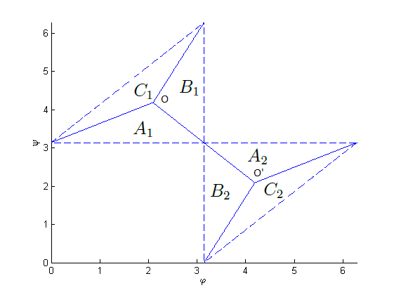 Figure 1
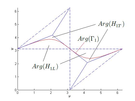 Figure 2
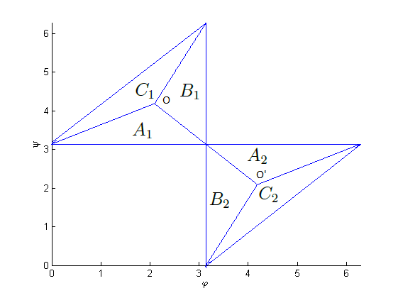 Figure 3
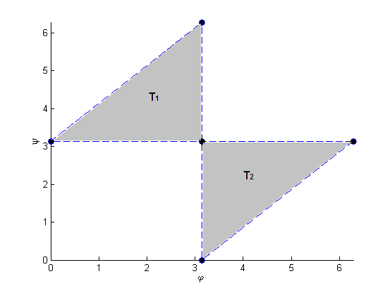 Figure 4
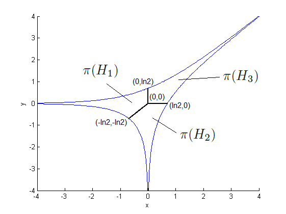 Figure 5
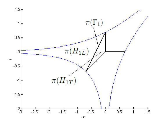 Figure 6
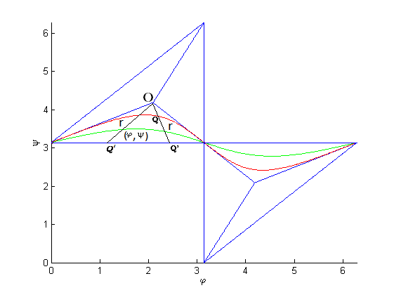 Figure 7
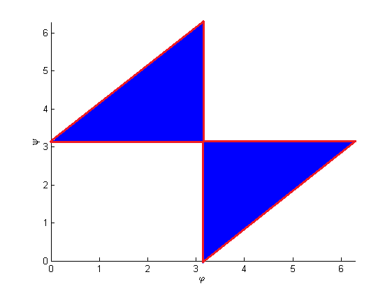 Figure 8
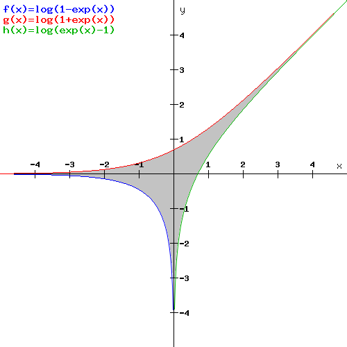 Figure 9
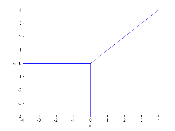 Figure 10
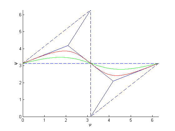 Figure 11