Correlations and entanglement of microwave photons emitted in a cascade decay
Simone Gasparinetti, Marek Pechal, Jean-Claude Besse, Mintu Mondal,, Christopher Eichler, and Andreas Wallraff

TL;DR
This paper demonstrates how a superconducting artificial atom can be coherently driven to produce correlated and entangled microwave photons through cascade decay, revealing new ways to generate entanglement in quantum microwave systems.
Contribution
It introduces a novel protocol using a superconducting atom to generate entangled microwave photons via cascade decay with phase-sensitive detection.
Findings
Successfully demonstrated phase correlation of emitted microwave photons
Generated entanglement between itinerant microwave modes
Highlighted the coherent nature of cascade decay in superconducting systems
Abstract
An excited emitter decays by radiating a photon into a quantized mode of the electromagnetic field, a process known as spontaneous emission. If the emitter is driven to a higher excited state, it radiates multiple photons in a cascade decay. Atomic and biexciton cascades have been exploited as sources of polarization-entangled photon pairs. Because the photons are emitted sequentially, their intensities are strongly correlated in time, as measured in a double-beam coincidence experiment. Perhaps less intuitively, their phases can also be correlated, provided a single emitter is deterministically prepared into a superposition state, and the emitted radiation is detected in a phase-sensitive manner and with high efficiency. Here we have met these requirements by using a superconducting artificial atom, coherently driven to its second-excited state and decaying into a well-defined…
Click any figure to enlarge with its caption.
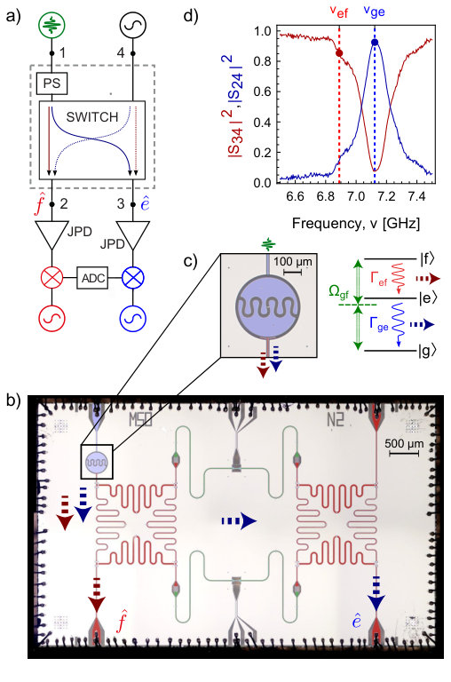 Figure 1
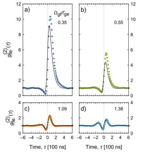 Figure 2
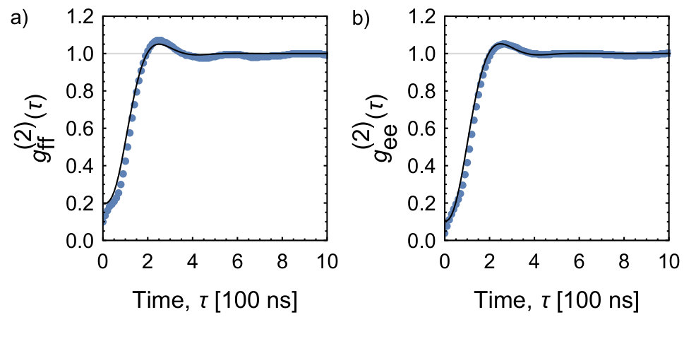 Figure 3
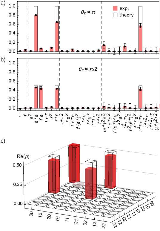 Figure 4
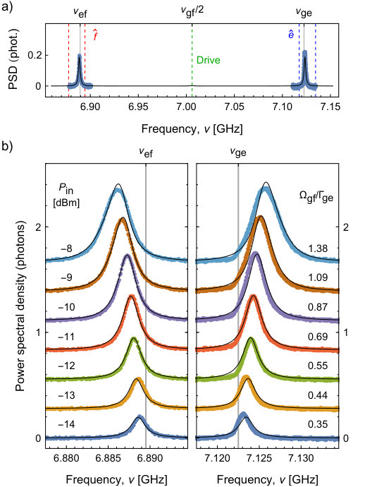 Figure 5
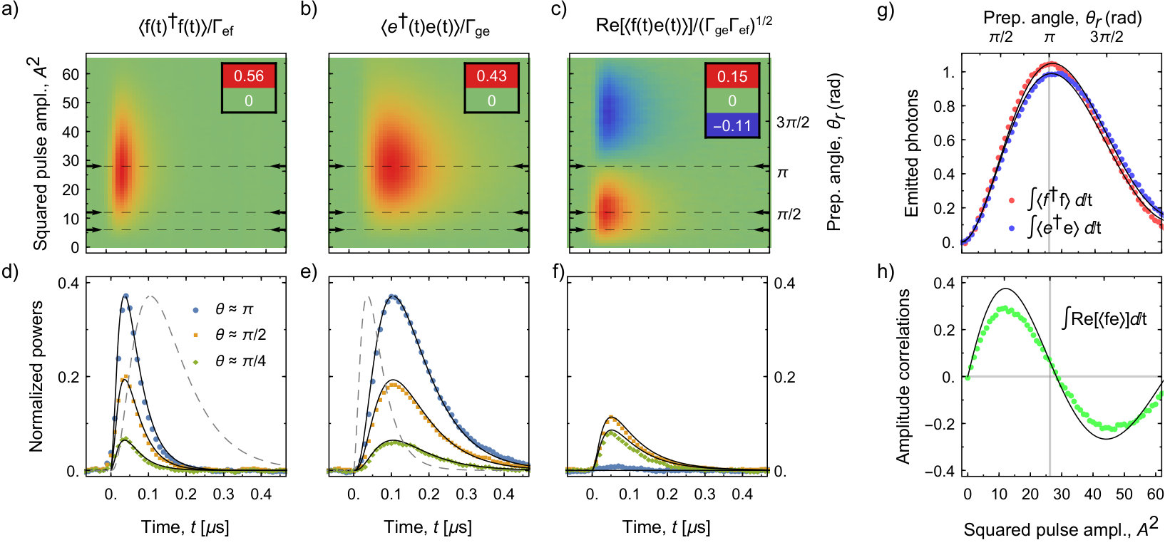 Figure 6
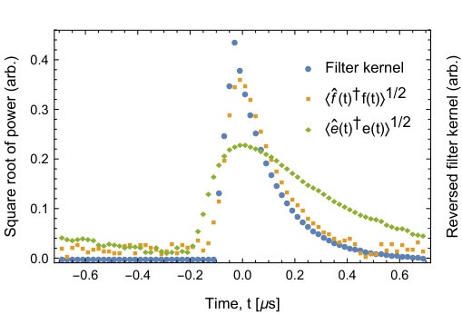 Figure 7
Peer Reviews
No public reviews on file for this paper yet. If you reviewed it on a platform where reviews are public (OpenReview, ICLR, NeurIPS, ICML), you can paste yours below so the community can read it here.
Videos
No videos yet. Explain this paper in a talk, walkthrough, or lecture? Add one.
Correlations and entanglement of microwave photons
emitted in a cascade decay
Simone Gasparinetti
Marek Pechal
Jean-Claude Besse
Mintu Mondal
Christopher Eichler
Andreas Wallraff
Department of Physics, ETH Zurich, CH-8093 Zurich, Switzerland
**An excited emitter decays by radiating a photon into a quantized mode of the electromagnetic field, a process known as spontaneous emission Loudon (2000). If the emitter is driven to a higher excited state, it radiates multiple photons in a cascade decay. Atomic Freedman and Clauser (1972); Aspect et al. (1981) and biexciton cascades Benson et al. (2000); Akopian et al. (2006); Stevenson et al. (2006); Dousse et al. (2010); Müller et al. (2014) have been exploited as sources of polarization-entangled photon pairs. Because the photons are emitted sequentially, their intensities are strongly correlated in time, as measured in a double-beam coincidence experiment Clauser (1974); Loudon (1980). Perhaps less intuitively, their phases can also be correlated, provided a single emitter is deterministically prepared into a superposition state, and the emitted radiation is detected in a phase-sensitive manner and with high efficiency. Here we have met these requirements by using a superconducting artificial atom, coherently driven to its second-excited state and decaying into a well-defined microwave mode. Our results highlight the coherent nature of cascade decay and demonstrate a novel protocol to generate entanglement between itinerant field modes. **
We have realized a photon source (Fig. 1) based on a transmon-type qubit Koch et al. (2007); Sathyamoorthy et al. (2016), with two lowest transitions at and between the ground, , the first excited, , and the second excited state, , and a resulting anharmonicity . The transmon is driven via a weakly coupled input port Peng et al. (2016); Pechal et al. (2016) and decays into one of the two input ports of the single-pole, double-throw switch described in Ref. Pechal et al. (2016), with a measured rate . The switch has a tunable center frequency, which we set to , and a bandwidth of . Photons of frequency () fall within (out of) the switch bandwidth and are routed from the source to output mode () [Fig. 1(a)]. Each output mode is amplified using a nearly-quantum-limited Josephson parametric dimer (JPD) Eichler et al. (2014) and its two quadratures are measured by heterodyne detection. We characterize the scattering properties of the switch by driving it via its second input port [Fig. 1(d)]. On this basis, we estimate that our routing scheme has an efficiency of () for photons of frequency ().
We first investigate the cascade decay of our source under continuous-wave excitation. We coherently drive the two-photon transition between and , with frequency [level scheme in Fig. 1(c)]. We vary the input power and analyze the spectrum of the scattered radiation (Fig. 2). Contributions from coherent (Rayleigh) scattering at the drive frequency are discarded in our detection chain. At low powers, the spectrum shows a single peak at each of the transition frequencies and . The photon flux into each mode, as given by the integrated power spectrum, first increases with power and then saturates as population is transferred into . At the same time, the two emission frequencies Stark-shift away from each other due to the driving of the two-photon transition Koshino et al. (2013). The measured data are in excellent agreement with a model based on a Lindblad-type master equation and input-output theory (solid lines, see Methods). The Rabi frequency describing coherent oscillations between and is proportional to the drive strength squared, i.e., directly proportional to , because we are driving a two-photon transition.
Further insight into the emitted radiation is provided by its statistical properties Bozyigit et al. (2011); da Silva et al. (2010); Eichler et al. (2012a); Lang et al. (2013). The power autocorrelation functions of the two modes, and , show that the emitted radiation is antibunched SM , a clear signature of single-photon emission Bozyigit et al. (2011); Hoi et al. (2012); Peng et al. (2016). Here, however, we focus on correlations between the two photons, as expressed by the normalized power cross-correlation function . A positive (negative) time delay corresponds to a photon being emitted in mode after (before) a photon is emitted in mode . At the lowest drive powers [Fig. 2(a,b)], shows antibunching at negative time delays () and strong superbunching at positive ones (), as expected for two time-correlated emissions occurring in a given sequence Clauser (1974); Loudon (1980). This pattern changes at higher powers [Fig. 2(c,d)], specifically, when the pump rate becomes comparable to the decay rates (). Due to fast repopulation of the level, there is an increased probability for the reverse sequence to occur, which results in a superbunching peak appearing at negative time delays. More generally, develops oscillations at frequency , revealing the coherent nature of the population transfer between and . The observed properties are captured well by our model (solid lines), which has no free parameters and takes the detection bandwidth of our setup into account (see Methods).
To characterize the radiation emitted in a single cascade, we use a preparation pulse, whose time envelope is a truncated Gaussian of variance and controlled amplitude . The pulse drives coherent oscillations between and , ideally preparing the transmon in the state , where is the preparation angle. The optimal pulse duration is determined by a tradeoff between decay during state preparation and spectral overlap with the neighboring transitions at and , which are direct single-photon transitions. We monitor the emitted radiation by performing ensemble averaging on the relevant moments of and da Silva et al. (2010); Eichler et al. (2012a).
We first consider the instantaneous powers and , whose time dependence corresponds to the temporal shapes of the emitted photons [Fig. 4(a,d) and (b,e)]. The two shapes differ from each other: the power in the mode reaches its maximum at an earlier time and decays faster than in the mode. These features are explained by considering that (i) the decay rates into the two modes are different by a factor , due to the dipole matrix elements of the transmon Koch et al. (2007), and (ii) while the state is directly populated by the excitation pulse, the state is initially empty: the two photons decay sequentially. The integrated powers, proportional to the photon numbers in each mode, oscillate as a function of the pulse amplitude squared [Fig. 4(g)]. These oscillations reflect those in the prepared -state population, to which both photon numbers are proportional. We fit our data to a master equation simulation taking into account the time dependence of the preparation pulse as well as radiative decay during preparation [Fig. 4(g), solid lines], and use the fit to determine the preparation angle as a function of the pulse amplitude .
We next consider the relative phase between the two photons. The amplitude-amplitude correlation is generally nonzero, indicating a well-defined relative phase [Fig. 4(c,f) and (h)]. The correlation is largest when the source is prepared in an equal state superposition (), and smallest when it is prepared in an energy eigenstate (). By contrast, we have verified that the individual mode amplitudes and vanish identically, regardless of the pulse amplitude. We interpret the observed results in terms of a mapping of the transmon state into two itinerant photonic modes, and . These modes are defined (and measured) by integrating the signals and over weighted time windows corresponding to the temporal shape of the emitted photons (temporal mode matching) Eichler et al. (2011a) (see Methods). In a Hilbert space comprising the transmon as well as the two modes, the cascade decay is described by the transformation
[TABLE]
where and indicate Fock states of the two modes with photon numbers zero and one. Equation (1) stands for an entangling operation in which the superposition state created in the transmon is eventually shared by the two modes.
We fully characterize the two modes by performing joint tomography on them Eichler et al. (2011a, 2012a) for the preparation angles and [Fig. 5(a-b)]. The measured moments are referred to the two outputs of the switch using the calibration procedure described in the Methods. The vanishing of first-order moments indicates that the radiation in each mode has no definite phase. Photon-photon phase correlations manifest themselves in the amplitude correlation, , which is substantial for a pulse and vanishes for a pulse. The single-photon nature of the radiation is confirmed by the vanishing of the fourth-order moments, and . Given the measured values for the moments and their respective standard deviations, we also determine the most likely density matrix describing the two modes at the output of the switch Welsch et al. (1999); Eichler et al. (2012a); Lang et al. (2013). For a pulse [Fig. 5(c)], we obtain a fidelity to the Bell state , and a negativity .
Our work demonstrates that in spite of its sequential nature, cascade decay must be regarded as a fully coherent process generating phase coherence between the emitted photons. Our excitation scheme can be extended to other architectures and generalized to multi-photon cascades and multiple modes. The ability to generate entanglement between spatially separated, itinerant radiation fields Eichler et al. (2011b); Flurin et al. (2012); Menzel et al. (2012); Lang et al. (2013); Peng et al. (2015); Lähteenmäki et al. (2016), as demonstrated in our experiment, is essential to quantum information distribution protocols.
Methods
Experimental details. Measurements are carried out in a dilution refrigerator at 35 mK. The measured device is the same as in Ref. Pechal et al. (2016). The frequency of the transmon and the working point of the switch are set by magnetic-flux tuning, for which we use two on-chip flux lines and a superconducting coil mounted underneath the chip. The transition frequencies and linewidth of the transmon are measured by low-power spectroscopy. In Fig. 1(d), the measurement of the scattering parameters is referenced to a detuned configuration of the switch in order to compensate for frequency-dependent attenuation and gain in the measurement lines. In Fig. 2, power spectral densities are measured as Fourier transforms of the autocorrelation functions of the two signals. In Fig. 3, power correlations are measured by double heterodyne detection followed by real-time signal processing prior to ensemble averaging Bozyigit et al. (2011); da Silva et al. (2010); Lang et al. (2013). The noise added by each detection chain is characterized by measuring its statistical properties with the drive tone turned off, and subtracted from the signal using the methods described in Refs. da Silva et al. (2010); Eichler et al. (2012a). Our detection bandwidths are set by the bandwidth of the parametric amplifiers and by the digital filter applied to the signals. In the measurements of Fig. 2, the detection bandwidth is for both modes. In those of Fig. 3, it is for both modes (limited by digital filtering). In those of Fig. 4, it is for mode and for mode (limited by the parametric amplifiers). The measurements of Fig. 5 are taken by integrating the two output signals with an appropriate mode-matching filter. Due to technical reasons, we are restricted to using the same filter for both channels; we therefore define a filter whose shape is intermediate between that of the two modes [as determined from Fig. 4(d,e)], and optimize the delay between the integration windows (see also the Supplementary Material SM ).
Theoretical modeling. Our model is based on a Lindblad-type master equation for a driven, ladder-type, three-level system coupled to a semi-infinite transmission line. The ratio between the dipole moments of the – to the –transition is taken to be Koch et al. (2007). The output fields and their correlations are calculated using input-output theory Walls and Milburn (2008) and the quantum regression theorem Carmichael (2002). More details can be found in the Supplementary Material SM .
Data analysis. In Fig. 2, the measured spectra are globally fit to our model, the only fit parameter being the total attenuation of the drive line (input 1 in Fig. 1).
In Fig. 3, we incorporate the finite detection bandwidth by convolving the calculated with the squared kernel of the used digital filter twice. This is an approximation that holds in the limit of low signal-to-noise ratio relevant here; for more details, see Ref. Lang (2014).
In Fig. 4(g), the solid lines are obtained by numerically solving the master equation with a time-dependent drive whose envelope matches our preparation pulse, and using the solution to calculate the integrated powers in the two modes as a function of the pulse amplitude. We fit the theory to the data and extract the conversion factor between pulse amplitude and drive strength, which we use to estimate the preparation angle . To model the data of Fig. 4(d-f), we assume (for simplicity) instantaneous state preparation of the transmon at time . We first calculate the two-time correlation functions , with , and then convolve these functions with Lorentzian kernels corresponding to the measured detection bandwidths.
The moments in Fig. 5(a,b) are reconstructed as explained in Ref. Eichler et al. (2012a) and referred to the outputs of the switch by applying global scaling factors to them. According to the master equation simulation described in the Supplementary Material SM , a preparation angle results in an average photon number of in both modes. After taking into account inefficient signal routing due to photon leakage into input port 1 (, see Ref. Pechal et al. (2016)) and imperfect frequency selectivity of the switch [see Fig. 1(d)], we estimate photon numbers and at the output of the switch, which we have used to scale the moments shown in Fig. 5. This scaling corresponds to total detection efficiencies for mode and for mode , which we believe to be limited by cable losses, noise added by the amplifiers, and imperfect temporal mode matching (see also Supplementary Information SM ). The error bars in Fig. 5(a,b) are determined as the standard deviation of 20 repeated measurements, each of which was averaged 64M times. In Fig. 5(c), we estimate the most likely density matrix using the algorithm described in Ref. Eichler et al. (2012a) and applied, for instance, in Ref. Lang et al. (2013). We restrict the Hilbert space to up to two photons in each mode.
In the Supplementary Figure S1, the data are corrected for weak thermal background radiation during the reference (“off”) measurements Lang et al. (2013); Eichler et al. (2015). The correction corresponds to a thermal population in mode and in mode .
Supplementary Information
I Supplementary data
I.1 Photon antibunching
In Fig. S1 we present measurements of the normalized power autocorrelation functions for the modes and , with , taken under the same experimental conditions as the measurements of Fig. 2(d). Both functions exhibit clear antibunching, in a similar way as previously observed for single-photon sources Bozyigit et al. (2011). Differently from single-photon emission by a two-level system, here we observe a flattening of the first-order derivative at small time delays. This effect, captured by our theory, is due to small oscillations in the autocorrelation functions, smoothed out by our digital filter.
II Theoretical model
II.1 Master equation
Our model is based on a master equation for a driven, ladder-type, three-level system coupled to a transmission line. The system Hamiltonian in a frame rotating at the drive frequency and after the rotating-wave approximation is
[TABLE]
where is the detuning of the drive from the bare two-photon transition frequency, is the drive strength, and is the relative strength between the two dipole transitions. For the transmon, Koch et al. (2007). We write the master equation for the density matrix of the transmon as . The Liouvillian is given by
[TABLE]
where is the decay rate of into the transmission line. We have also introduced a total annihilation operator comprising the individual annihilation operators for the two transitions, , and , and the dissipator is expressed in the standard form
[TABLE]
II.2 Analytic expression for the Rabi frequency
We consider the unitary evolution given by the Hamiltonian (S1) in the limit and with . The evolution operator can be expressed analytically in terms of roots of a cubic equation. For a given , we seek the optimal detuning that maximizes the visibility of oscillations between states and . We find that unit visibility is attained for . This frequency shift from the bare two-photon resonance is an ac-Stark shift induced by the driving field. The corresponding Rabi frequency is given by , up to second order in the small parameter . Numerical simulations confirm that this approximation is accurate in the power range expored in our experiment, for which .
II.3 Input-output theory
Because the detection bandwidth of modes and is much smaller than the frequency difference between the two transitions (anharmonicity), we assume that the transmon decays from into by emitting a photon into the mode (with rate ), and from to into mode (with rate ). The mode operators are thus given by
[TABLE]
II.4 Continuous excitation
To model the response under continuous excitation, we first find the steady-state that satisifes . We calculate the power spectral density of the emitted radiation for each mode (in units of photon flux per unit frequency, or simply photons) as the Fourier transform of the corresponding autocorrelation function:
[TABLE]
The normalized power cross correlation between the modes is given by Carmichael (2002)
[TABLE]
II.5 Pulsed excitation
The full dynamics of the system under pulsed excitation is obtained from a numerical solution of the master equation generated by (S2), with a time-dependent drive strength . To obtain analytical expressions for the time dependence of the field moments, we take the limit of instantaneous state preparation and assume that at time the transmon is prepared in the state . Using Eqs. (S4), we find that the amplitudes of each mode identically vanish: and at all times. The instantaneous powers read
[TABLE]
In both modes, the power is proportional to the initial -state population . In mode , the power is maximum at the time of preparation and decays exponentially as the state decays into with rate . The nonmonotonic time dependence of the power in mode stems from two competing effects, as the emitting state , initially empty, is both populated by the decay from and depleted by the decay into . As a result, the maximum power is reached at the delayed time . Furthermore, the decay in mode is slower by a factor . To obtain the number of photons radiated into each mode, we integrate the two expressions and find
[TABLE]
The amplitude correlation between the two channels reads
[TABLE]
We note that this correlation is maximum at , despite the fact that the state is empty at that time. The integrated correlation reads
[TABLE]
The dependence of the integrated quantities on the Rabi angle is consistent with the coherent mapping of the state of the three-level system into two itinerant bosonic modes, according to Eq. (1) in the main text.
III Experimental details
III.1 Loss in detection efficiency due to imperfect temporal mode matching
For each time-dependent mode (with ), we define the corresponding temporally matched, time-independent mode as , where the mode-matching function satisfies the normalization condition .
In our experiment, temporal mode matching is achieved by convolving the digitized signals with a finite-impulse response (FIR) filter and recording the result of the convolution at the time that maximizes the signal. Recalling the definition of convolution, one sees that the kernel of the filter corresponds to a time-reversed sampling of at the digitization rate of the acquisition system. The optimal filter kernels for the two modes can be estimated from the measured shapes of the emitted photons [Fig. 4 and S2]. Due to the way our digital acquisition card is configured, here we are restriced to using the same filter for both modes. Imperfect mode matching results in a decrease in the overall detection efficiencies for the two modes. It does not, however, alter the statistical properties of the modes Eichler et al. (2012b). We estimate the detection efficiency due to mode matching by convolving the filter with the square root of the measured photon shape. For the optimal filters, . For the used filter, for mode and for mode .
The reference list from the paper itself. Each links out to its DOI / PubMed record.
- 1Loudon (2000) R. Loudon, The Quantum Theory of Light , 3rd ed. (Oxford University Press, 2000).
- 2Freedman and Clauser (1972) S. J. Freedman and J. F. Clauser, Phys. Rev. Lett. 28 , 938 (1972) . · doi ↗
- 3Aspect et al. (1981) A. Aspect, P. Grangier, and G. Roger, Phys. Rev. Lett. 47 , 460 (1981) . · doi ↗
- 4Benson et al. (2000) O. Benson, C. Santori, M. Pelton, and Y. Yamamoto, Phys. Rev. Lett. 84 , 2513 (2000) . · doi ↗
- 5Akopian et al. (2006) N. Akopian, N. H. Lindner, E. Poem, Y. Berlatzky, J. Avron, D. Gershoni, B. D. Gerardot, and P. M. Petroff, Phys. Rev. Lett. 96 , 130501 (2006) . · doi ↗
- 6Stevenson et al. (2006) R. M. Stevenson, R. J. Young, P. Atkinson, K. Cooper, D. A. Ritchie, and A. J. Shields, Nature 439 , 179 (2006) . · doi ↗
- 7Dousse et al. (2010) A. Dousse, J. Suffczynski, A. Beveratos, O. Krebs, A. Lemaitre, I. Sagnes, J. Bloch, P. Voisin, and P. Senellart, Nature 466 , 217 (2010) . · doi ↗
- 8Müller et al. (2014) M. Müller, S. Bounouar, K. D. Jons, M. Glassl, and P. Michler, Nat Photon 8 , 224 (2014) . · doi ↗