On The Feasibility of Exomoon Detection Via Exoplanet Phase Curve Spectral Contrast
Duncan H. Forgan

TL;DR
This paper investigates the potential for detecting exomoons through spectral contrast in exoplanet phase curves, highlighting the challenges and conditions under which such detection might be feasible with current or future telescopes.
Contribution
It provides a parameter survey showing the difficulty of detecting exomoons via phase curves and identifies conditions like tidal heating that could make detection possible with advanced instruments.
Findings
Most exomoon signals are undetectable with current observations.
Detection requires photometric precision of 10 ppm or better.
Self-luminous moons could be detectable at wavelengths > a few microns.
Abstract
An exoplanet-exomoon system presents a superposition of phase curves to observers - the dominant component varies according to the planetary period, and the lesser varies according to both the planetary and the lunar period. If the spectra of the two bodies differs significantly, then it is likely there are wavelength regimes where the contrast between the moon and planet is significantly larger. In principle, this effect could be used to isolate periodic oscillations in the combined phase curve. Being able to detect the exomoon component would allow a characterisation of the exomoon radius, and potentially some crude atmospheric data. We run a parameter survey of combined exoplanet-exomoon phase curves, which show that for most sets of planet-moon parameters, the lunar component of the phase curve is undetectable to current state-of-the-art transit observations. Even with future…
Click any figure to enlarge with its caption.
 Figure 1
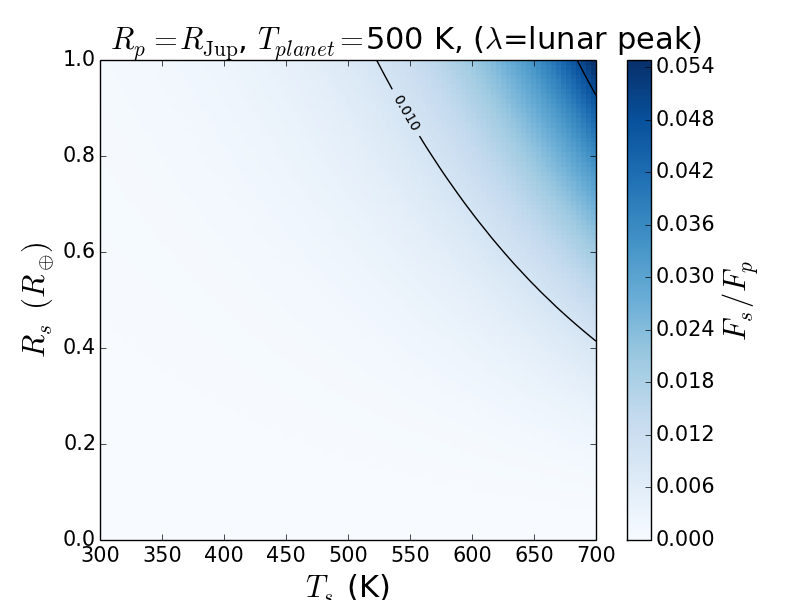 Figure 2
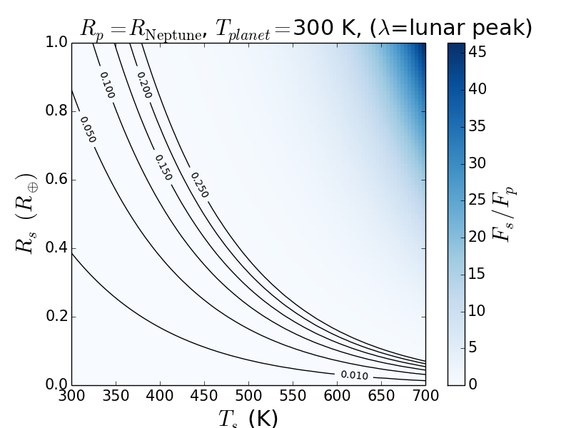 Figure 3
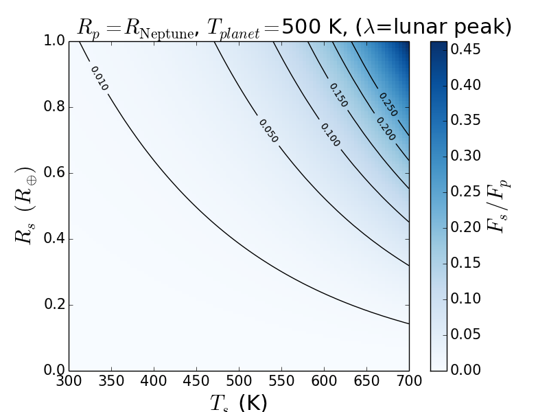 Figure 4
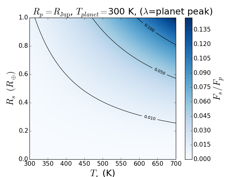 Figure 5
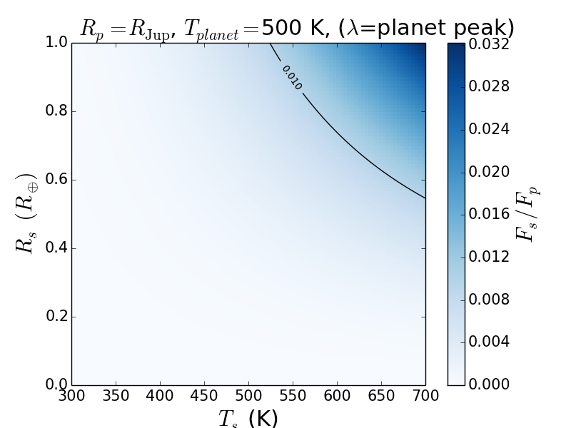 Figure 6
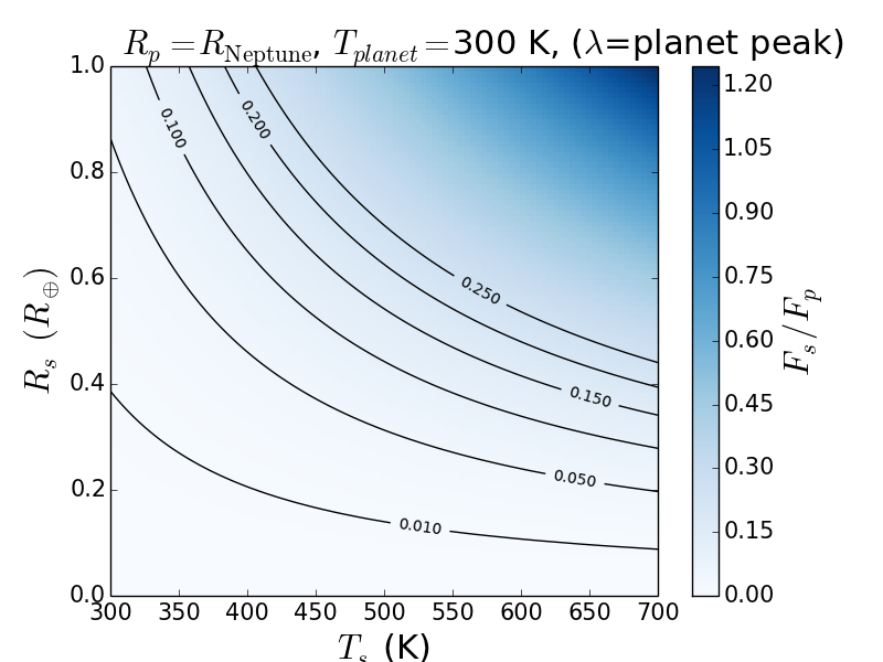 Figure 7
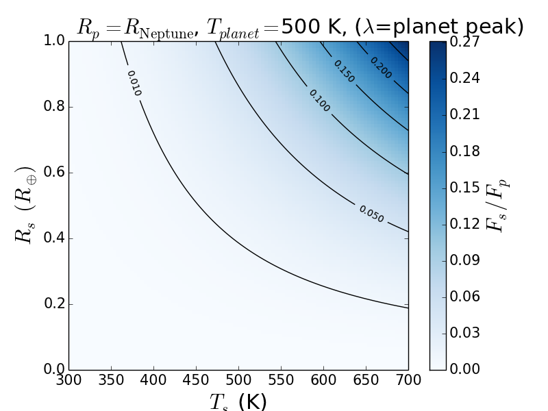 Figure 8
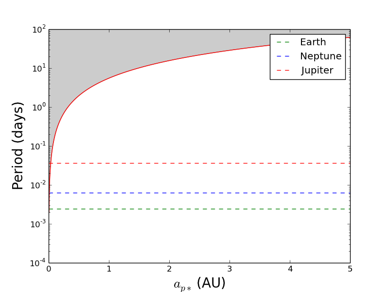 Figure 9
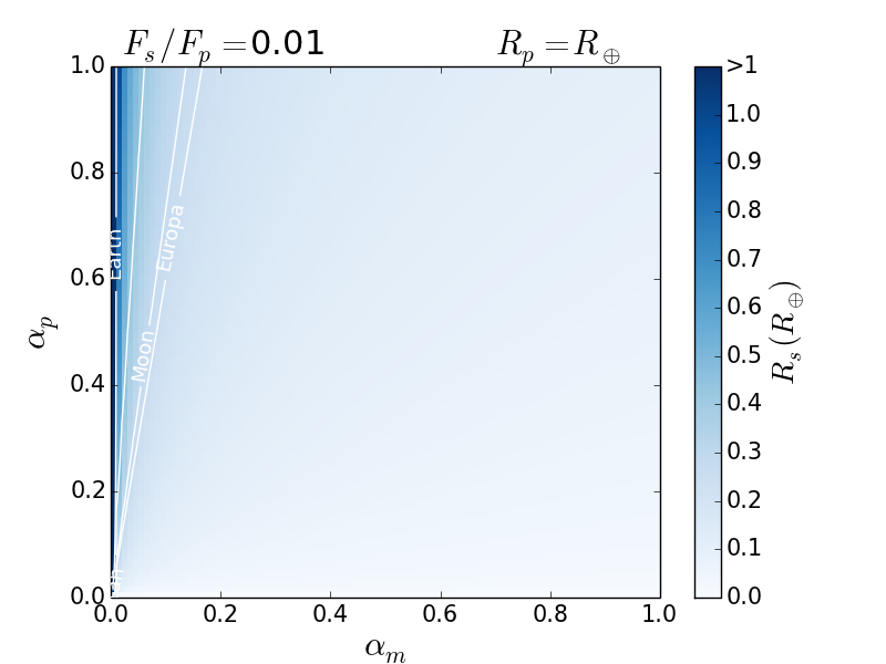 Figure 10
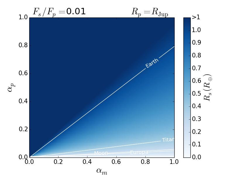 Figure 11
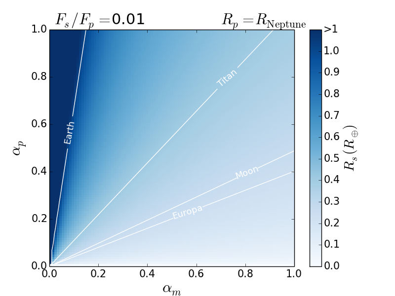 Figure 12
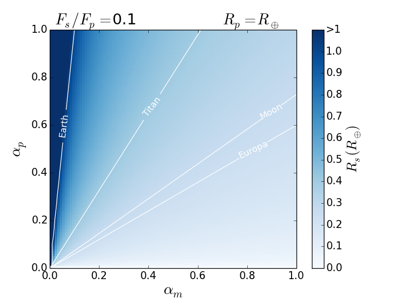 Figure 13
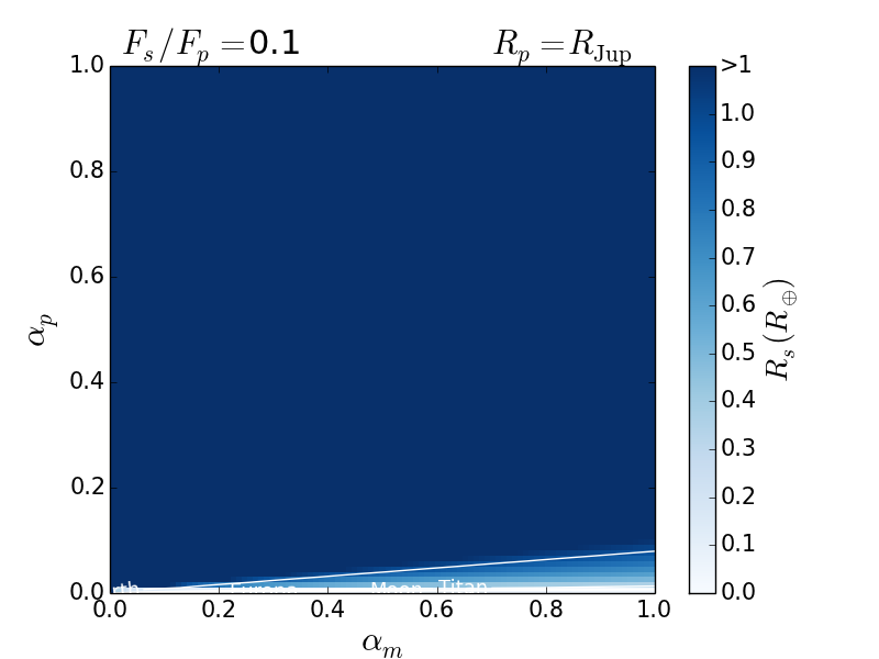 Figure 14
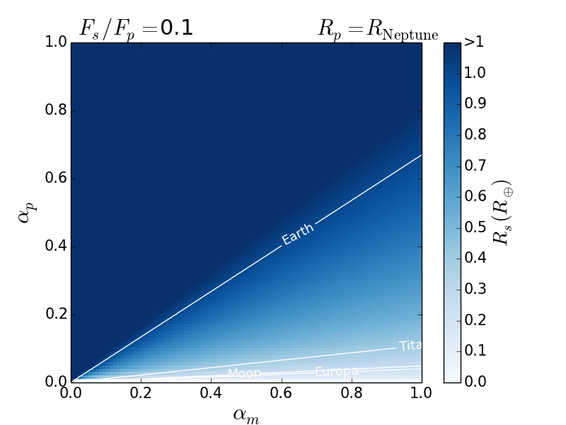 Figure 15
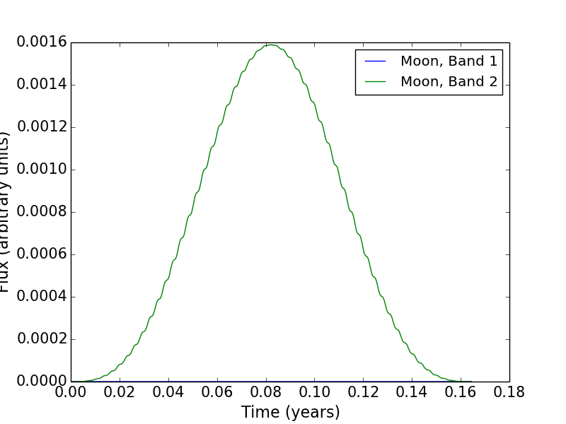 Figure 16
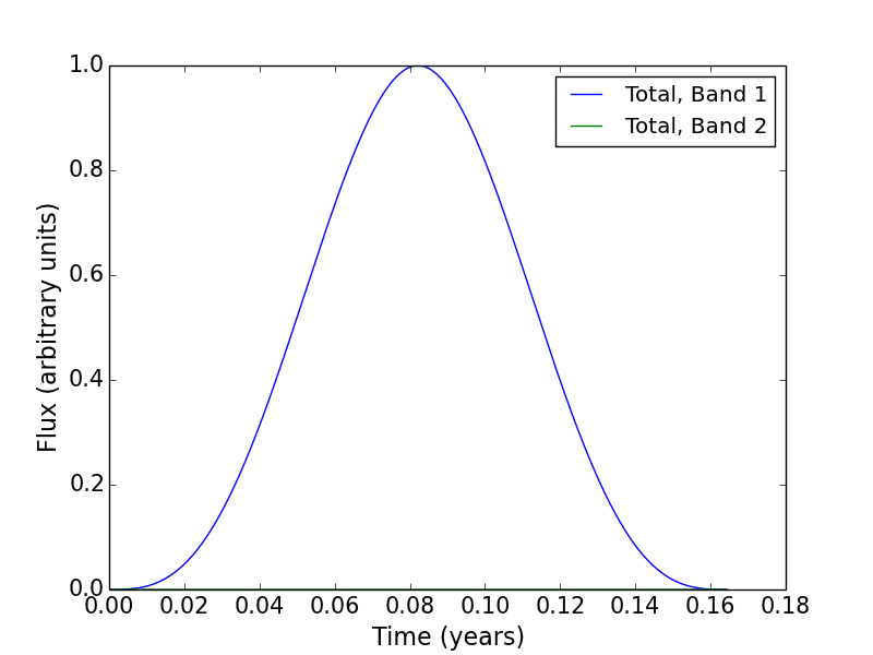 Figure 17
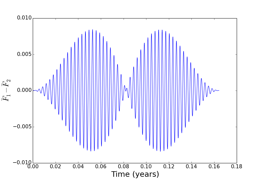 Figure 18
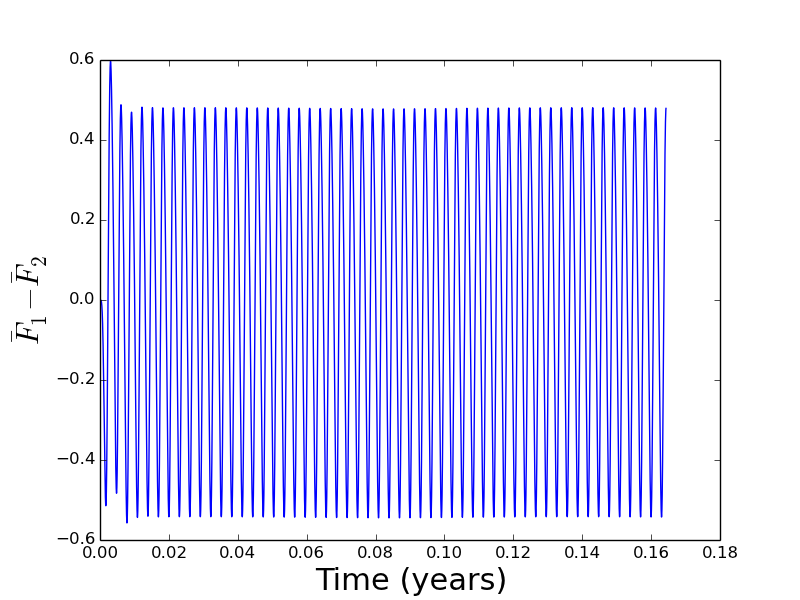 Figure 19
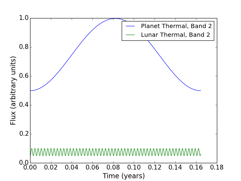 Figure 20
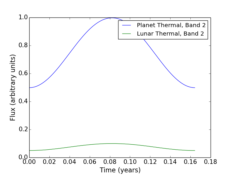 Figure 21
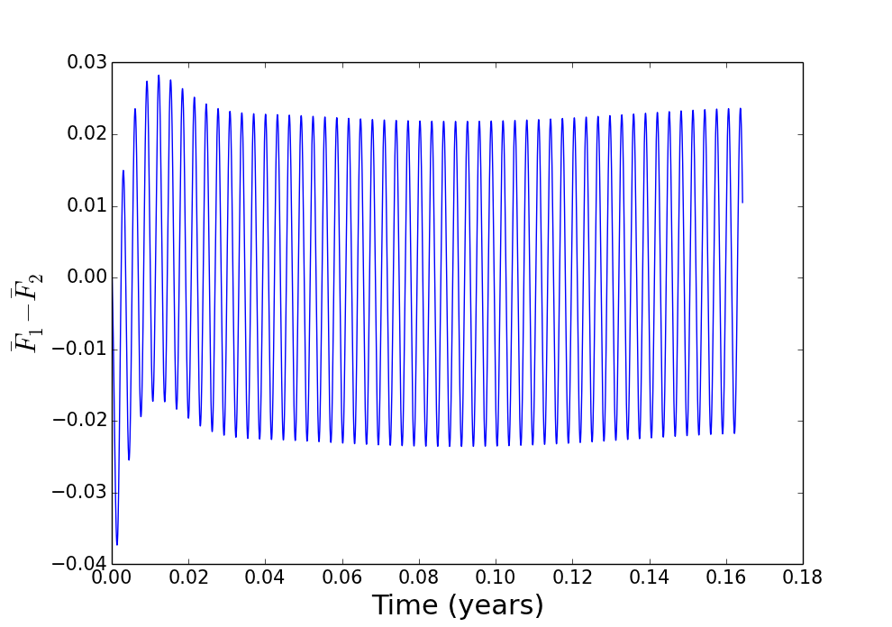 Figure 22
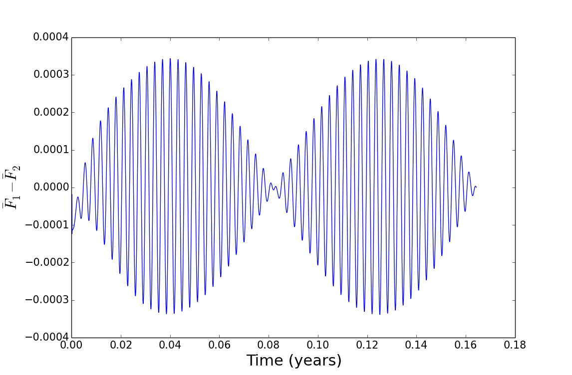 Figure 23
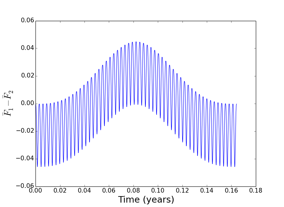 Figure 24
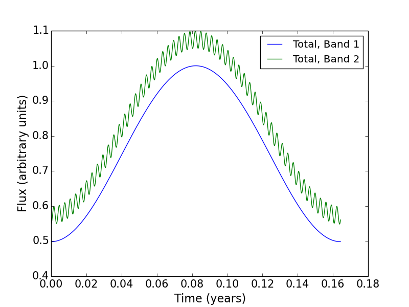 Figure 25
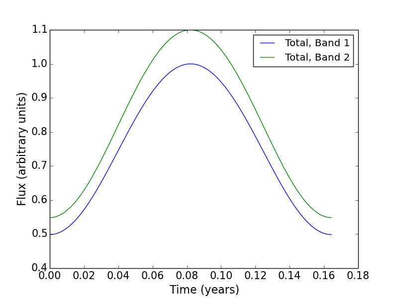 Figure 26
Peer Reviews
No public reviews on file for this paper yet. If you reviewed it on a platform where reviews are public (OpenReview, ICLR, NeurIPS, ICML), you can paste yours below so the community can read it here.
Videos
No videos yet. Explain this paper in a talk, walkthrough, or lecture? Add one.
On The Feasibility of Exomoon Detection Via Exoplanet Phase Curve Spectral Contrast
D. H. Forgan1,2
1SUPA, School of Physics & Astronomy, University of St Andrews, North Haugh, St Andrews, Scotland, KY16 9SS, UK
2St Andrews Centre for Exoplanet Science Contact e-mail: [email protected]
(Accepted XXX. Received YYY; in original form ZZZ)
Abstract
An exoplanet-exomoon system presents a superposition of phase curves to observers - the dominant component varies according to the planetary period, and the lesser varies according to both the planetary and the lunar period. If the spectra of the two bodies differs significantly, then it is likely there are wavelength regimes where the contrast between the moon and planet is significantly larger. In principle, this effect could be used to isolate periodic oscillations in the combined phase curve. Being able to detect the exomoon component would allow a characterisation of the exomoon radius, and potentially some crude atmospheric data.
We run a parameter survey of combined exoplanet-exomoon phase curves, which show that for most sets of planet-moon parameters, the lunar component of the phase curve is undetectable to current state-of-the-art transit observations. Even with future transit survey missions, measuring the exomoon signal will most likely require photometric precision of 10 parts per million or better.
The only exception to this is if the moon is strongly tidally heated or in some way self-luminous. In this case, measurements of the phase curve at wavelengths greater than a few microns can be dominated by the lunar contribution. Instruments like the James Webb Space Telescope and its successors are needed to make this method feasible.
keywords:
planets and satellites: detection, general, atmospheres
††pubyear: 2016††pagerange: On The Feasibility of Exomoon Detection Via Exoplanet Phase Curve Spectral Contrast–On The Feasibility of Exomoon Detection Via Exoplanet Phase Curve Spectral Contrast
1 Introduction
While the detection of extrasolar planets (exoplanets) continues apace111http://exoplanets.eu, the detection of their satellites, extrasolar moons or exomoons remain undetected. This is not for want of trying - several teams are attempting to achieve this first detection. The community has been able to deliver strong upper limits on the sizes of exomoons in their samples (see e.g. Kipping et al. 2015), and these constraints are expected to grow tighter in the coming years as the exoplanet transit missions CHEOPS (Simon et al., 2015) and PLATO (Hippke, 2015) come online.
This lack of exomoon detections is also not for want of exomoon detection methods. The recent literature abounds with indirect and direct techniques. Some examples include transit timing and duration variations (TTVs/TDVs) (Sartoretti & Schneider, 1999; Simon et al., 2007; Kipping, 2009a, b; Lewis, 2013; Heller et al., 2016a), direct transits of exomoons (e.g. Brown et al. 2001; Pont et al. 2007; Dobos et al. 2016), microlensing events (Han & Han, 2002; Bennett et al., 2014), mutual eclipses of directly imaged planet-moon systems (Cabrera & Schneider, 2007) or mutual eclipses during a stellar transit (Sato & Asada, 2009). Averaging of multiple transits may also yield an exomoon signal, either through scatter peak analysis (Simon et al., 2012) or orbital sampling of light curves (Heller et al., 2016b). In the radio, emission from giant planets may be modulated by the presence of moons within or near the magnetosphere (Noyola et al., 2014), or indeed by moon-induced plasma torii (Ben-Jaffel & Ballester, 2014).
Many of these methods are relatively agnostic to the wavelength of the observation. Some very recent proposals for detection methods rely on differences in the spectra of the planet and moon. For example, the spectro-astrometric detection method proposed by Agol et al. (2015) attends to directly-imaged exoplanet-exomoon systems. Direct imaging lacks the spatial resolution to separately image the moon - however, comparing observations at two wavelengths can identify a shift in centroid, if one wavelength happens to coincide with a regime where the planet is faint and the moon is bright. For example, an icy moon is generally quite reflective across a variety of wavelengths, but a giant planet may contain significant (and relatively wide) absorption features (such as the methane feature at around 1.4 ).
We consider a new, but related spectral detection method. Photometric observations of transiting exoplanets across a full orbital period obtain primary and secondary transits (where the planet eclipses the star and the star eclipses the planet respectively), and the phase curve, a smoothly varying component which increases as the planet’s dayside comes in and out of view (see e.g. Winn, 2011; Madhusudhan & Burrows, 2012). The phase curve’s period is that of the planet’s orbit around the star. Any exomoons present will also make contributions to the phase curve. These contributions will have multiple components, whose periods are equal to the planetary orbital period and the lunar orbital period (depending on the radiation budgets of both bodies).
In principle, if there are regions of the spectrum where the contrast between the moon and planet is high, the exomoon’s phase curve may be isolated by subtracting the modelled exoplanet phase curve, if it is measured at multiple wavelengths. In essence, we are searching for a periodicity in the total phase curve that can only be explained by the presence of an exomoon.
We investigate the efficacy of this detection method, which we christen phase curve spectral contrast (PCSC). This concept builds on the work of Robinson (2011)222In fact, the genesis of this idea may be traced as far back as Williams & Knacke (2004) and Selsis (2004), who considered the time-dependence of the Earth-Moon’s combined spectrum, and advocated a phase differencing between e.g. full phase and quadrature. The technique discussed here is similar, but we focus less on the Earth-Moon system, and consider a more generalised approach, with a consequently larger parameter space. We also attempt to use the entire phase curve, rather than two instantaneous measurements.
Moskovitz et al. (2009) also presented a detailed study of the Moon’s effect on the Earth’s infrared phase curve using both a 1D energy balance model and a 3D general circulation climate model, but these results were focused on a single wavelength of observation (see also Gómez-Leal et al. 2012’s use of real atmospheric data in a similar study). Multi-frequency observations will be crucial for detections, especially in the absence of detailed knowledge of the atmospheric properties of each body.
This paper is structured as follows: in section 2 we motivate this detection method by considering how spectral contrast can assist in extracting exomoon’s contribution to the phase curve, and we describe code we have written to investigate the phase curves produced by exoplanet-exomoon systems; in section 3 we give examples of the combined phase curves produced in a series of limiting cases, and consider the exomoon parameter space that could be probed by this detection method given present and future transit surveys; finally in section 4, we summarise the work.
2 Analytical Description
We can write the flux received from an exoplanet, as the sum of reflected stellar radiation and the planet’s thermal radiation:
[TABLE]
where is the stellar flux, is the planet’s albedo, is the planetary radius, is the semimajor axis of the planet’s orbit, and is the planet’s thermal flux. We can write a similar equation for the lunar flux, :
[TABLE]
The lunar flux now includes reflective contributions from the star and the planet respectively. In the limit that , we can approximate . Expanding and rearranging gives:
[TABLE]
and thus we can write the contrast ratio
[TABLE]
To clarify matters, let us consider some limiting cases. Firstly, in the limit that the thermal contribution of both bodies is negligible, we obtain
[TABLE]
The right hand term is likely to be negligible, so we then derive the following reflectivity contrast condition for the moon/planet flux contrast to be significant:
[TABLE]
This defines our detection limit for non-luminous planets and moons. In the limit that thermal emission dominates, the flux contrast ratio becomes:
[TABLE]
In this limit, we must rely on the moon being significantly more luminous than the planet (perhaps due to tidal heating effects, cf Peters & Turner 2013; Dobos & Turner 2015).
So what exomoons might contrast methods be amenable to? It is interesting to note that there is no direct relation to in either of our detection limits. For example, a transiting planet at large semimajor axis with a young, hot moon may be amenable to these methods, or an extremely low-albedo planet (although the planet’s own phase curve, and subsequent spectral contrast, will of course be affected by distance to the star). We will investigate the detailed parameter space in the following sections.
2.1 Computing Combined Exoplanet-Exomoon Phase Curves
For simplicity, we will assume that both the exoplanet and the exomoon orbit their host with zero eccentricity, and that both bodies orbit within the plane. Their orbital motions are simply
[TABLE]
Where we define the orbital longitudes as:
[TABLE]
The star is fixed at the origin. An observer is placed along the y-axis. The phase curve of each body depends on the angle between the emitter and the observer, from the perspective of the emission recipient . We have three emitter-recipient pairs in the system: star-planet, star-moon and planet-moon, and at any given instant we must compute three angles , where
[TABLE]
We assume both the exoplanet and exomoon possess isotropically scattering Lambertian surfaces, ensuring both bodies have fully analytic phase curves (the reader can find detailed numerical integrations of phase curves for other scattering laws in Madhusudhan & Burrows 2012). The phase function in this case is
[TABLE]
We compute the total flux received at time as follows. Firstly, we compute the stellar flux reflected by the planet:
[TABLE]
and the same for the moon:
[TABLE]
We then compute the thermal flux from both bodies. We fix a flux difference between the night and day side of each body (relative to the star) , and assume the flux from each side is isotropic. Consequently, we can use a simple cosine function to describe the fraction of dayside visible to the observer (Williams & Gaidos, 2008):
[TABLE]
We can then immediately write the planet’s thermal flux
[TABLE]
To write the same equation for the satellite, we must know what defines the dayside nightside contrast on the moon, i.e. is the lunar temperature governed by stellar or planetary flux? If the lunar terminator is determined by stellar flux, the resulting phase curve will possess similar time variation to the reflective case. If the lunar terminator is determined by planetary flux, then the lunar’s thermal contribution to the phase curve will vary according to the lunar period about the planet, presenting a wholly different signal. The two cases are (respectively):
[TABLE]
Note that we have neglected the moon’s thermal flux variation due to the planet’s orbit about the star. Finally, we compute the planetary flux reflected by the moon, which will combine both reflected starlight and thermal planetary radiation:
[TABLE]
In the second term, we account for the moon receiving changing levels of thermal radiation from the planet as it passes between the day side and the night side. This is described by the angle between the stellar and lunar position vectors, relative to the planet position vector:
[TABLE]
2.2 Extracting Lunar Signals from the Phase Curve
Essentially, our task is to extract a short period signal from a combined signal containing a variety of periods. If the planet’s mass and semimajor axis are well characterised, then we can focus our search to regions of period space where an exomoon may stably orbit.
The orbital stability limits for a moon around a planet are defined by the Roche limit at low exomoon semimajor axis, and the Hill Stability criterion at large exomoon semimajor axis. The inner Roche limit for an exomoon is:
[TABLE]
By application of Kepler’s third law, the corresponding lunar orbital period is:
[TABLE]
The outer stability limit is proportional to the planet’s Hill radius :
[TABLE]
where (Domingos et al., 2006). Again, this can be converted to an orbital period:
[TABLE]
The minimum and maximum permissible orbital periods as a function of planet mass and semimajor axis can be found in Figure 1.
Two approaches are possible. If the exomoon contribution in a single band is very strong, we can bandpass filter the combined exoplanet-exomoon phase curve (at a given wavelength) for signals inside the period range , where we must assume a priori to obtain the lower limit. We should expect to be significantly lower than 333if the planet and moon masses are comparable, the produced transit signals will be markedly different, see Lewis et al. 2015. Computing the generalised Lomb-Scargle periodogram (GLS, Zechmeister & Kürster, 2009; Mortier et al., 2015) of this filtered signal can then identify promising oscillations. The second approach requires simultaneous measurements of the phase curve in two wavelength bands (one where the planet dominates, and one where the moon dominates). This can permit a successful subtraction of the exoplanet phase curve to return a periodic residual, which can then be analysed via the GLS periodogram.
3 Tests & Discussion
3.1 The Highly Reflective Regime
As an illustration, we first consider a system containing a star, a planet orbiting at 0.3 au (orbital period yr). We place a Europa-like moon in a circular orbit around the planet, with size , and orbital semimajor axis au.
We consider measurements made in two bands, and hence with two different albedos for each object. The planetary albedo , and the satellite’s albedo . These are extreme values, which we select for illustrative purposes only.
The top row of Figure 2 shows the contributions from the phase curve due to the planet, and due to the moon, in both bands. In Band 1, the exomoon contribution is virtually nil, and hence the total phase curve is indistinguishable from that of the exoplanet phase curve. In Band 2, the albedo ratio , which greatly exceeds the size ratio . The total phase curve is now dominated by the exomoon, which we can see in the top right panel of Figure 2.
To isolate the periodic signal of the exomoon, we normalise the curve in each band by its mean:
[TABLE]
We compute , and then pass this quantity through a bandpass filter to remove trends much longer than the lunar period (i.e. of order the planetary period), the results of which are displayed in the bottom left panel of Figure 2. We can perform this filtering with confidence, as we know the maximum permissible lunar orbital period from dynamical stability arguments (Figure 1). Note the amplitude modulation of the curve, which is characteristic of a planet-moon system. If the moon had orbited the star, and not the planet, we would instead receive the steady-amplitude signal shown in the bottom right panel of Figure 2.
We provide this example to illustrate the reflective limit of our calculations, but the effect strength is so small it is unlikely to ever be usable for detecting Galilean analogues, as we will see in the following section. This technique may be more amenable to Earth-Moon analogues, where the satellite-planet size ratio is much higher, and the albedo ratio between the Moon and Earth is relatively high, given a judicious choice of wavelength. This has already been demonstrated by Robinson (2011) and Gómez-Leal et al. (2012) in detail, and we will show more general constraints in the following section.
3.2 Detection Limits
So what can we expect to observe in the highly reflective limit? If we specify a given moon-planet flux ratio that we believe observations can detect, then we can rearrange equation (5) to obtain the detectable moon-planet size ratio:
[TABLE]
By considering detection limits in terms of , we have implicitly assumed that the exoplanet phase curve is itself detectable. In effect, we now ask: to what level of precision is the exoplanet phase curve known? Is this precision sufficient to yield a periodic signal indicative of a highly reflective exomoon? Conversely, we should also consider what levels of are insufficient to detect exomoons of a given radius or radius ratio. We address the absolute detection limits considering current and future surveys, and sources of intrinsic phase curve variability in section 3.5.
Figure 3 shows the detectable moon radius, as a function of and (assuming that we can characterise the phase curve to precisions of at least 10% (left column) or 1% (right column)). Note that these limits are independent of , but they are ultimately not encouraging.
Being able to characterise an exoplanet phase curve with uncertainties below 1% is a formidable challenge. If we are only able to characterise the curve to within 10%, then we are unlikely to detect moons below orbiting a planet (unless we can identify wavelength regimes where and ). If the planet is Neptune-sized, then the limits on are much less constraining, and Titan-sized moons come within grasp if is large. In the terrestrial regime a wide range of parameter space becomes available (although the measurement of the exoplanet phase curve itself becomes significantly more challenging).
We should therefore conclude that for the present time, moons that are not self-luminous are unlikely to be detected around giant planets using this method (at least for some time), although there may be promising regions of parameter space for Neptunes and super-Earths. It is also worth noting that the planet TrES-2b has an extremely low measured geometric albedo of (Kipping & Spiegel, 2011). A highly reflective sub-Earth radius moon in this system would be detectable even with 10% precision in the phase curve.
3.3 The Highly Thermal Regime
We now investigate the nature of the highly thermal regime by reducing the albedo of both bodies in all bands to . We set the thermal flux from the planet to be constant across both bands, and set the ratio of thermal fluxes from both bodies in each band to be . For both objects, we set the ratio of thermal flux from the day and night side . Figure 4 shows the individual contributions to the phase curve generated by the planet and moon. The left column indicates the curves generated if the lunar thermal flux is determined by the star, and the right column shows the case where the lunar thermal flux is determined by the planet. We also show the normalised subtraction for both cases, and the equivalent subtraction if the moon was in fact orbiting the star (Figure 5).
If the star determines the lunar thermal flux, the exomoon curve’s principal period is the planetary period, in much the same fashion as the reflective case. The residuals derived from the normalised subtraction (top plot in Figure 5) are also extremely similar to those found for the reflective case, despite the change from a reflective Lambertian phase function to a dayside visibility function.
If the planet determines the lunar thermal flux, the exomoon curve’s principal period is the lunar period, as we are most sensitive to the surface variation of flux as the moon moves in and out of view. The combined phase-curve is a simple superposition of the exoplanet and exomoon periods, and the normalised subtraction (middle plot in Figure 5) is a simple sinusoid, which is easily distinguished from the case where both bodies orbit the star (right panel). However, this is extremely similar to the two-planet residual in the highly reflective limit (Figure 2). Determining would be required to break degeneracy in this case.
3.4 Detection Limits
As we did for the highly reflective regime, we can rearrange equation (7) to obtain the minimum detectable size ratio as a function of the flux ratio and physical parameters, although we will also have to specify the planetary and lunar thermal fluxes to do so. If we assume that both the planet and moon are blackbody emitters, then
[TABLE]
Where are the effective temperatures of the two bodies. The critical size ratio for detection depends on the peak wavelength of emission for the satellite:
[TABLE]
If we assume that both bodies are in thermal equilibrium with the stellar radiation field, then
[TABLE]
where and are the Bond albedo of planet and satellite respectively. As before, we approximate , and hence
[TABLE]
In other words, if the stellar radiation field dominates the lunar energy budget, it is likely that and hence the detectability of such moons is difficult (except if the planetary Bond albedo is unusually high and the lunar Bond albedo is unusually low).
Of course, the temperature of the moon may not be determined by the stellar radiation field. If the exomoon is strongly tidally heated, then it may well be that the moon surface temperature is significantly higher than the planet’s regardless of albedo444This depends heavily on the redistribution of heat from the lunar dayside to the lunar nightside. Even with strong tidal heating, effective heat redistribution will result in very low variations of thermal flux between dayside and nightside. Figure 6 shows the detectability of tidally heated exomoons around a Jupiter-radius planet by phase curve spectral contrast as a function of moon temperature and (Figure 7 shows the same for a Neptune-sized planet). In both cases, the planets orbit an M star at AU, and the lunar semimajor axis is fixed at AU (the resulting lunar detection limits are insensitive to both parameters, but the planet’s detection is more likely for reduced ). We consider two different planetary temperatures: 300K and 500K.
We also consider measurements made either at the wavelength corresponding to the Wien peak of the planet’s blackbody emission, or the Wien peak of the moon, given . Measuring at the moon’s peak clearly is best for detection of lunar photons, but measuring at the planet’s peak is best for characterising the planetary phase curve in detail. As we have seen in previous sections, comparing measurements of planet-dominated and lunar-dominated bands is the key to this detection method.
For Jupiter-sized planets at 500K (), even extremely hot moons have a low contrast of at the planetary peak. Shifting to shorter wavelengths allows these hot moons to have a boosted contrast (top right plot of Figure 6). For example, a 1 moon at would constitute around 25% of the total phase curve signal.
If the planet has a temperature of 300 K, then the moon is more detectable even at wavelengths tuned to the planet’s peak (). At lunar-tuned wavelengths, the emission from a 850K moon dominates the phase curve signal, even for satellites as small as 0.2 !
Neptune-sized planets offer even better prospects, especially at . A Titan-sized body only needs to achieve a temperature of around 500K to begin dominating the lunar-tuned band (while still achieving in the planet-tuned band).
What is less clear is the expected phase curve from tidally heated bodies. The temperature difference between day and night sides of a synchronously rotating, tidally heated moon is clearly a function of local rheology, and how tidal heat is redistributed from the interior.
Finally, we should note that we have assumed a blackbody spectrum for the planet in this section. A planet with strong absorption bands longward of a few would provide even better contrast to moons experiencing extreme tidal heat.
3.5 Prospects for plausible measurements with current/future instruments
To determine what values of we can expect to constrain in the future, let us begin with current calculations of the detectability of the phase curve of a single exoplanet in transit surveys.
Consider a transit survey with a duration given by baseline , and cadence . If we are attempting to detect a signal with amplitude over one epoch of its period , the signal-to-noise ratio is
[TABLE]
where is the photometric precision. We introduce a factor of to accomodate the fact we are dealing with a sinusoidal signal rather than a step function. If we are able to observe the maximum number epochs of the signal within , then the combined signal-to-noise
[TABLE]
If we are attempting to detect the phase curve induced by a single exoplanet (in the highly reflective regime), then
[TABLE]
And hence the signal to noise ratio is
[TABLE]
We can immediately check the detectability with the Kepler space telescope by substituting (i.e. the entire Q0-Q17 baseline), , and per six-hour timebin, where we have assumed our putative sample is in the upper tenth percentile of Kepler stars () to obtain this precision (Christiansen et al., 2012). This gives
[TABLE]
As we can see, this limited sensitivity rules out Earth-sized planets possessing detectable phase curves, let alone any potential moons. If we consider instead a Jupiter-sized planet orbiting at AU, then
[TABLE]
As is independent of , we can obtain the of an exomoon phase curve by simply multiplying by . To maintain , say, we are only able to probe signals of
[TABLE]
If the exomoon’s phase curve was generated purely by reflection, this would require . For extreme tidal heat, Earth-sized satellites may be detectable around warm Jupiters and Neptunes, but the satellite must have a surface temperature well in excess of 600 K (see the bottom right plots in Figures 6 and 7).
This establishes the phase curve oscillation method as being of very limited use for current state-of-the art transit surveys. We can now ask: what criteria must a transit survey satisfy in order for this technique to become feasible?
The cadence of future transit surveys (such as TESS, CHEOPS and PLATO), is typically of order 1 minute, although the photometric precision for TESS is likely to be worse (see e.g. Rauer et al., 2014; Sullivan et al., 2015; Simon et al., 2015).
Let us now consider a putative survey where , with a similar to Kepler. We can rearrange to obtain the required photometric precision for detection with :
[TABLE]
For a relatively high amplitude exomoon signal of , then we must still demand a photometric precision of around 10 ppm, which is extremely difficult to achieve. Failing this, we must then demand extremely long baselines .
It is also worth pointing out that our analysis has assumed white noise. Correlated noise, instrumental systematics and the stellar activity inherent to the target will impose a floor on the possible precision. This is significantly worse if the periodicity of the stellar activity is close to either the planetary or lunar periods. We have also assumed that the planet itself does not show intrinsic brightness variations due to weather or other sources of atmospheric variability (cf Esteves et al., 2013; Webber et al., 2015; Armstrong et al., 2016).
On the other hand, binning of the data can help ameliorate systematics/activity, but this still requires long observing campaigns (and inappropriate bin sizes will destroy any lunar signal). Binning also introduces an implicit dependence on the planetary period, as the effective improvement from binning a data train of fixed length is diminished for longer periods.
If our moon is tidally heated, then it is possible that , but this is typically at wavelengths much longer than the typical visible/near IR bands used for exoplanet transit surveys, and will probably require space-based observatories. The natural candidate is the James Webb Space Telescope (Greene et al., 2016; Batalha et al., 2017), and/or the future LUVOIR (Bolcar et al., 2016) and HabEx missions (Gaudi & Habitable Exoplanet Imaging Mission Science and Technology Definition Team, 2017).
4 Conclusions
We have investigated the feasibility of analysing exoplanet phase curves to determine if there is an extra component produced by an exomoon, a technique we christen exomoon phase curve spectral contrast (PCSC). This technique relies on multiple frequency measurements of the curve, and isolating frequencies where the moon is relatively bright compared to the planet, which can be the case at specific infrared frequencies where the planet’s atmosphere is in absorption.
We find that in general, phase curve measurements will have to be extremely precise to detect even modest satellite-to-planet size ratios. We calculate that for this technique to detect exomoons, a photometric precision of 10 ppm or smaller is required, while maintaining cadences of order 1 minute. If the moon is strongly tidally heated, lower precisions may be sufficient, but will require observations at wavelengths greater than .
This technique is similar to the spectro-astrometric method of Agol et al. (2015) in that both require measurements in multiple bands where different components of the system dominate, but is complementary in that Agol et al. (2015)’s method works for high-contrast direct imaging, not transits. It also bears a resemblance to the mutual events detection method of Cabrera & Schneider (2007) - their method also uses direct imaging, but relies on observing a lunar transit or eclipse. These events are quite short in time (of order a few hours), and hence very high cadence measurements are required over much longer campaigns, compared to PCSC. Importantly, in contrast to both Agol et al. (2015) and Cabrera & Schneider (2007), PCSC does not require individual targeting of sources, and can be directly applied to exoplanet transit survey data, given appropriate precision.
Exomoon detection for transiting exoplanets is perhaps more likely to proceed from e.g. transit timing and duration variation measurements (TTVs/TDVs), which typically rely on Bayesian inference to determine the moon’s properties (e.g. Kipping, 2011), and can probe satellite-to-planet mass ratios as low as depending on the object (Kipping et al., 2015). The additional information obtained from measuring the phase curve can assist in informing the priors that enter these calculations, and could reduce the permitted solution space for exomoon orbital and structural parameters, although not by much until photometric precisions improve.
As this technique is most suited to tidally heated exomoons, studying exoplanet phase curves for exomoon contributions will place stronger constraints on the existence of high temperature satellites of planets orbiting relatively cool stars.
Acknowledgements
DHF gratefully acknowledges support from the ECOGAL project, grant agreement 291227, funded by the European Research Council under ERC-2011-ADG. The author warmly thanks David Armstrong, Andrew Collier-Cameron, Ian Dobbs-Dixon, David Kipping, Joe Llama, Annelies Mortier and Hugh Osborn for stimulating discussions, and Tyler Robinson for an insightful review of this manuscript. This research has made use of NASA’s Astrophysics Data System Bibliographic Services.
The reference list from the paper itself. Each links out to its DOI / PubMed record.
- 1Agol et al. (2015) Agol E., Jansen T., Lacy B., Robinson T. D., Meadows V., 2015, Ap J , 812, 5 · doi ↗
- 2Armstrong et al. (2016) Armstrong D. J., de Mooij E., Barstow J., Osborn H. P., Blake J., Saniee N. F., 2016, Nature Astronomy , 1, 0004 · doi ↗
- 3Batalha et al. (2017) Batalha N. E., et al., 2017, PASP, p. in press
- 4Ben-Jaffel & Ballester (2014) Ben-Jaffel L., Ballester G. E., 2014, Ap J , 785, L 30 · doi ↗
- 5Bennett et al. (2014) Bennett D., et al., 2014, Ap J , 785, 155 · doi ↗
- 6Bolcar et al. (2016) Bolcar M. R., Feinberg L., France K., Rauscher B. J., Redding D., Schiminovich D., 2016, in Mac Ewen H. A., Fazio G. G., Lystrup M., Batalha N., Siegler N., Tong E. C., eds, Proceedings of the SPIE. p. 99040 J, doi:10.1117/12.2230769 , %****␣exomoon_PCO.bbl␣Line␣50␣****http://proceedings.spiedigitallibrary.org/proceeding.aspx?doi=10.1117/12.22%30769 · doi ↗
- 7Brown et al. (2001) Brown T. M., Charbonneau D., Gilliland R. L., Noyes R. W., Burrows A., 2001, Ap J , 552, 699 · doi ↗
- 8Cabrera & Schneider (2007) Cabrera J., Schneider J., 2007, Astronomy and Astrophysics , 464, 1133 · doi ↗