Tensorial dynamics on the space of quantum states
J. F. Cari\~nena, J. Clemente-Gallardo, J.A. Jover-Galtier, G., Marmo

TL;DR
This paper presents a geometric tensorial framework for describing the dynamics of quantum states and their evolution under Markovian processes, enabling analysis of nonlinear quantities like entropy and concurrence.
Contribution
It introduces a novel geometric formulation using tensor fields to model quantum state evolution and Markovian dynamics in a unified, natural way.
Findings
Tensorial formulation describes Markovian evolution as a vector field on state space
Allows analysis of nonlinear physical quantities such as entropy and concurrence
Identifies limits leading to contraction of Jordan and Lie products
Abstract
A geometric description of the space of states of a finite-dimensional quantum system and of the Markovian evolution associated with the Kossakowski-Lindblad operator is presented. This geometric setting is based on two composition laws on the space of observables defined by a pair of contravariant tensor fields. The first one is a Poisson tensor field that encodes the commutator product and allows us to develop a Hamiltonian mechanics. The other tensor field is symmetric, encodes the Jordan product and provides the variances and covariances of measures associated with the observables. This tensorial formulation of quantum systems is able to describe, in a natural way, the Markovian dynamical evolution as a vector field on the space of states. Therefore, it is possible to consider dynamical effects on non-linear physical quantities, such as entropies, purity and concurrence. In…
Click any figure to enlarge with its caption.
 Figure 1
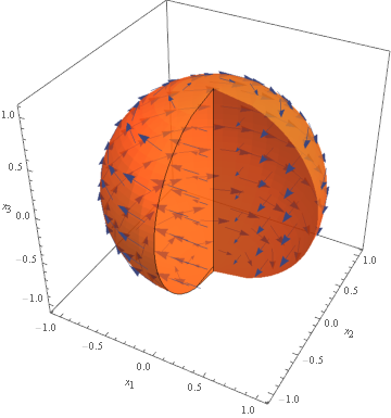 Figure 2
Peer Reviews
No public reviews on file for this paper yet. If you reviewed it on a platform where reviews are public (OpenReview, ICLR, NeurIPS, ICML), you can paste yours below so the community can read it here.
Videos
No videos yet. Explain this paper in a talk, walkthrough, or lecture? Add one.
Tensorial dynamics on the space of quantum states
J.F. Cariñenaa), J. Clemente-Gallardoa,b), J.A. Jover-Galtiera,b), G. Marmoc,d).
*a)*Departamento de Física Teórica, Facultad de Ciencias, Universidad de Zaragoza.
c. Pedro Cerbuna 12, 50.009 Zaragoza, Spain.
*b)*Instituto de Biocomputación y Física de Sistemas Complejos (BIFI).
c. Mariano Esquillor (Edificio I+D), 50.018 Zaragoza, Spain.
*c)*Dipartimento di Fisica, Università degli Studi di Napoli Federico II.
Via Cintia, 80.126 Napoli, Italy.
*d)*INFN, Sezione di Napoli. Via Cintia, 80.126 Napoli, Italy.
Abstract: A geometric description of the space of states of a finite-dimensional quantum system and of the Markovian evolution associated with the Kossakowski-Lindblad operator is presented. This geometric setting is based on two composition laws on the space of observables defined by a pair of contravariant tensor fields. The first one is a Poisson tensor field that encodes the commutator product and allows us to develop a Hamiltonian mechanics. The other tensor field is symmetric, encodes the Jordan product and provides the variances and covariances of measures associated with the observables. This tensorial formulation of quantum systems is able to describe, in a natural way, the Markovian dynamical evolution as a vector field on the space of states. Therefore, it is possible to consider dynamical effects on non-linear physical quantities, such as entropies, purity and concurrence. In particular, in this work the tensorial formulation is used to consider the dynamical evolution of the symmetric and skew-symmetric tensors and to read off the corresponding limits as giving rise to a contraction of the initial Jordan and Lie products.
PACS: 02.40.Yy, 03.65.Vf, 03.65.Yz.
Mathematics Subject Classification: 81P16, 81Q70.
Keywords: quantum systems; density states; geometric formalism; algebra contraction; master equation.
1 Introduction
In the last forty years there has been a widespread interest in a geometrical description of quantum phenomena analogous to the Hamiltonian description of classical mechanics. Most of the approaches have been done in the the Schrödinger picture of pure states, or equivalently, of the dynamics of quantum pure states described by Landau-von Neumann equation [1, 2, 3, 4, 5, 6, 7, 8, 9, 10, 11, 12]. In this setting, the complex Hilbert space associated to a quantum system is identified with a real differentiable manifold endowed with a complex structure, i.e. a -tensor field that reproduces the complex linearity properties of . There also exists a canonical Kähler structure induced by the Hermitian inner product defining the Hilbert space structure, i.e. is a Kähler manifold. Similar considerations, using the natural projection, prove that the projective Hilbert space is also a Kähler manifold. Thus, the space of pure states of quantum systems is endowed with a geometric structure.
The other ingredients of a quantum system have to be also described in geometric terms: observables are represented by some functions on the manifold , whose values at each point are precisely the expectation values of the observables in the corresponding state of the system. The Schrödinger equation, which governs the unitary evolution of isolated systems, is represented by a vector field which is both a Hamiltonian and a Killing vector field with respect to the canonical Kähler structure on the complex projective space. For a complete presentation of this geometrical description, see the aforementioned references.
This study of dynamics of pure states in the Schrödinger picture is adequate to describe isolated physical systems. However, more realistic evolutions associated with open systems require a statistical analysis of dynamics. From this point of view, the states of quantum systems are described by density matrices [13, 14], which are convex combinations of projectors on one-dimensional subspaces of the Hilbert space. The state of the system is said to be pure if it corresponds to one of those projectors (or equivalently, a point in the complex projective space). Otherwise the state of the system is said to be mixed. Their corresponding density matrices are the required tool to understand the general behaviour of open quantum systems, i.e. systems whose evolution is influenced by an external environment whose properties can only, at most, be averaged.
Following the description of Hilbert and projective complex spaces in geometrical terms, this work aims to characterise geometrically the pure and mixed states of quantum systems, by extending some previous work done by some of us [15, 7, 16, 17], where a tensorial description of the set of observables (and its dual space ) was considered. Density matrices can be identified as -linear functionals acting on a complex unital C*-algebra , whose real elements represent the physical observables in the Heisenberg picture. These real elements form a real Lie-Jordan algebra . States are described by the subset of normalised, positive functionals of the dual space . It has been shown [18, 19] that, from the geometrical point of view, the set of states is a stratified manifold with a boundary, and a convex set whose extremal points are the pure states.
The geometric description of the dual space leads to the definition of a pair of tensor fields on , a symmetric one, (of Jordan type, in this case), and a skew-symmetric one, (the canonical Lie-Poisson structure on the dual of the Lie algebra). Similarly to the case of the Schrödinger picture, these tensor fields encode the relevant algebraic structures of the algebra of observables. In the present work, we will describe how those tensors of can be used to obtain another pair of tensors on the subset of states which will allow us to encode the Heisenberg formalism in tensorial language. Geometric tools can be thus employed in order to characterise the evolution of quantum systems. Among the advantages of the formalism, it is possible to study the change in non-linear properties, such as entropies or purity, or even more abstract ones, as the algebraic properties of quantum observables. This last feature will be dealt with in detail for the case Markovian systems.
Markovian dynamical maps were classified in the mid seventies by Gorini, Kossakowski, Sudarshan and coworkers [20, 21, 22], and by Lindblad [23]. The non-unitary evolution defined by the Kossakowski-Lindblad dynamics has some novel properties not present in the case of unitary evolutions. Some characteristics of the Kossakowski-Lindblad evolution, such as the existence and properties of limit states, have been studied by Zanardi [24], Baumgartner and coworkers [25, 26], Albert and coworkers [27] and many others (see references in those works). A complete geometric description of their properties is given in this paper. Thus, the vector field corresponding to the system of differential equations that determines the evolution is described by the sum of three vector fields: a Hamiltonian one, a gradient one and a third vector field associated with a Kraus-type action on the space of states. The definition of each one will become clear in the text. This geometrical characterisation allows us to consider the dynamics from a new perspective.
As an application of the method, we will reproduce in terms of tensor fields the contraction of algebras of observables presented in [28, 29, 64]. The theory of contractions of algebras was introduced in the 1950’s by I. E. Segal [30], E. Inönü and E. P. Wigner [31], and later extended by other authors [32, 33, 34, 35, 36, 37, 38, 39]. By a well-defined procedure that will be detailed below, it is possible to obtain new algebras from a given one by considering the asymptotic limit of a family of linear transformations of the algebra. This new algebra is called a contraction of the initial one. In the context of Quantum Mechanics, some types of evolutions may define contractions of the Lie-Jordan algebra of observables of the system. This is a relatively unknown topic that, nevertheless, may have interesting applications that will be studied in future works. The geometric formalism presented here is particularly well-suited for the description of contractions, since it allows to formulate them at the level of the observables and, at the same time, at the level of the quantum states. The results presented here may shed some light on the relevance of these contractions in the study of quantum systems.
The paper is organised as follows. Section 2 summarises some of the results presented in previous works, and focuses on the new tensorial approach to the dynamics on the space of states. Hence, instead of describing the dynamics on the whole dual space of the Lie-Jordan algebra of observables, we define tensor fields only on the stratified submanifold of states. Similarly, observables are no longer represented by linear functions, but by expectation value functions. The resulting geometrical objects are indeed physically relevant. The new functions are the correct way to represent observables on quantum systems, as their values are the results that can be obtained in measurements of quantum systems. On the other hand, the resulting tensor fields reproduce the properties of quantum systems. The new Poisson tensor fields is connected, as before, with the unitary evolution of quantum systems, while the symmetric one reproduces geometrically another important aspect of quantum systems: the variance and covariance of observables.
As an application of these results, in Section 3 a 2-level system is studied. The Hamiltonian and gradient vector fields are computed, and their integral curves are plotted to get some insight on the dynamics of states. In Section 4, we consider the new tensors in order to describe, in geometrical terms, the Kossakowski-Lindblad evolution. Section 5 presents the second main contribution of this paper: we consider Kossakowski-Lindblad evolution and prove that, in simple cases, we can consider its effect on the tensors and capture in this way a contraction of the algebra of observables of the quantum system. The last section of the paper, Section 6, is devoted to discuss the results presented in the paper and its relevance in the geometrical description of the dynamics of quantum systems.
2 The geometry of the set of quantum states
This section is concerned with the geometric description of the Heisenberg picture of Quantum Mechanics, which characterises physical quantum systems in a purely algebraic setting. In its modern formulation, the Heisenberg picture characterises the observables of a physical system as the real elements of a unital C*-algebra [40, 10, 41, 42, 43, 44, 45]. States of the system are normalised positive real -linear functionals on the C*-algebra. The evaluation of these functionals on observables represents the outcome of a measurement process.
It is possible to describe the Heisenberg picture in geometric terms [40, 18, 19]. This follows the path initiated by the aforementioned geometric description of the Schrödinger picture. Algebraic properties of the space of observables naturally define tensor fields on its dual space Observables themselves are represented by linear functions on this dual space. Thus, a geometric description of the algebra of observables is achieved by identifying the real vector space of observables and by introducing two product structures, the Lie and the Jordan brackets. We are obliged to do so because the associative product on the set of (complex) operators, when restricted to real elements is no longer an inner product. It breaks up into two different inner products, a skew symmetric one and a symmetric one, which define, respectively, a Lie product and a Jordan product.
However, a step further is required in order to truly obtain a geometric description of the Heisenberg picture. Not every element in represents a state of the quantum system. Thus, a geometric characterisation of the subset of states has to be done. As argued below, such a characterisation cannot be trivially related with the one obtained for . Instead, the relevant geometrical objects have to be redefined in order to admit a restriction to . In particular, observables are no longer represented by linear functions, but by expectation value functions. In this way, a proper description of the geometrical properties of the set of states is obtained.
A comment should be made regarding the dimensionality of quantum systems. In our analysis, we will restrict ourselves to finite-dimensional quantum systems, and hence to differentiable manifolds. The extension to general infinite-dimensional cases introduces so many topological subtleties that the new insight given by the geometrical encoding is obscured by the technical problems. Nonetheless, finite-dimensional quantum systems provide useful models to describe a huge number of physical problems, either exactly (such as spin systems and problems of quantum information) or by approximations (as by setting a limit to the energy of quantum systems with unbounded Hamiltonian). In any case, having in mind the possibility of developing a geometrical description of infinite-dimensional quantum systems in future works, statements will be presented, if possible, in a coordinate independent manner that can cover both cases of finite and infinite dimensions.
2.1 The Lie-Jordan algebra of observables
Definition 2.1**.**
A C-algebra is [46, p. 70] an involutive Banach (associative) algebra over the complex field , satisfying the condition*
[TABLE]
where denotes the norm and is an involution in which is also an antiautomorphism, i.e. an invertible antilinear map such that and . An element is said to be real if . The -linear subspace of real elements of will be denoted .
In the Heisenberg picture, one considers the C*-algebra of bounded operators on a Hilbert space, whose real elements are identified as the observables of the quantum system [47]. Real elements do not constitute an associative subalgebra, because the product of two real elements is not, in general, real. If the symmetrised product is considered instead, then a real element is obtained out of two real elements. Associativity, however, is lost. It is thus possible to introduce some appropriate new algebraic structures, which can be defined by using the associative product.
Definition 2.2**.**
Let be a Lie product on a linear space over a field (either or ), that is, a skew-symmetric -bilinear map from to that satisfies Jacobi identity,
[TABLE]
Let be a Jordan product on , that is, a symmetric -bilinear product satisfying Jordan identity,
[TABLE]
The pair is called a Lie algebra and the pair is called a Jordan algebra. The triple is called a Lie-Jordan algebra if, for each , is a derivation of the Jordan algebra , i.e. , and the associators of the Lie product and the Jordan product are proportional:
[TABLE]
for any and some real non-zero number .
Proposition 2.3**.**
Let be an -dimensional C-algebra with unity, and consider the following products defined in terms of the associative composition law in :*
[TABLE]
The product is a Lie bracket, while is a Jordan product. The triple , is a Lie-Jordan algebra over the field of real numbers .
Proof.
The set inherits the -linear structure of , and is a closed set under both products. The triple satisfies the axioms of Lie-Jordan algebras, which can be checked by direct computation. ∎
Remark 1*.*
The associative composition law in the C*-algebra is recovered as
[TABLE]
In particular, .
Further details in the description of Lie-Jordan algebras and their relevance in Quantum Mechanics can be found in books by G. Emch [46] and N. P. Landsman [48].
2.2 Tensorial description of the dual space of a Lie-Jordan algebra
It is possible to obtain a tensorial description of the algebraic properties of [40, 10, 18, 19]. This is achieved by considering the natural differentiable structure on the dual space of real -linear functionals on . Several geometrical objects on are related with relevant structures in the description of Quantum Mechanics. In particular, quantum observables are identified with linear functions on .
Definition 2.4**.**
Given an element , we denote by the evaluation function, i.e. the -linear function on defined by
[TABLE]
This is an injective -linear homomorphism of linear spaces, , which is an isomorphism for the finite-dimensional case.
Up to here we have replaced real elements of the –algebra (i.e., the physical observables) with linear functions on the dual space . We will denote as the set of these functions. Clearly the pointwise product of two linear functions will not be linear and therefore the corresponding structure will not be an inner product (i.e., the pointwise product of two evaluation functions is not an evaluation function). It is however possible to induce a Lie-Jordan structure on the space of linear functions. Being functions on a manifold we can also consider the corresponding differentials and their products and provide a tensorial realization of the algebraic structures of . Our experience with Lie algebras and their descriptions in terms of Poisson structures on the dual space suggests to define a pair of tensors, one symmetric and one skew-symmetric (and their corresponding brackets) to describe the Lie-Jordan algebra.
The linear structure of a vector space implies that both its tangent and cotangent bundles are trivialisable. In the particular case of the dual space , we have and . Unless necessary to distinguish, the same notation will be used for tangent vectors to and points in , on one side, and for covectors on and elements in , on the other. With this trivialisation, the Lie bracket and Jordan product on can also be given a geometrical description. They are represented by -tensor fields on , defined as follows.
Definition 2.5**.**
For any point , let be the two -bilinear maps defined, respectively, by the Jordan product and the Lie product on as follows
[TABLE]
for any pair .
Proposition 2.6**.**
Let and denote the sections of (the twice contravariant tensor bundle of ) such that , , for any point . Then, and are smooth - tensor fields.
Proof.
There are two equivalent ways of understanding smooth tensor fields [40]: either as smooth sections of tensor bundles, or as -linear maps on vector fields and 1-forms. Both and are, by definition, smooth sections of . Their -linearity is derived from the -linearity of the Lie bracket and the Jordan product, thus satisfying the requirements. ∎
The tensor field is the canonical Kirillov-Kostant-Souriau Poisson tensor field, while is a symmetric tensor field [18]. To compute their coordinate expressions, let us fix the notations for elements in the Lie-Jordan algebra and in its dual space . Assume that carries an inner scalar product, and consider an orthonormal basis for . An observable takes the form , with and where summation over repeated indices is understood. The composition laws in are determined by their structure constants and :
[TABLE]
where and . Let be the dual basis on , i.e. the set of linear functions on satisfying
[TABLE]
Any element can be decomposed in this basis as . Coordinate functions on with respect to the given basis are functions associated to the elements in the basis of :
[TABLE]
Coordinate functions on will be denoted as . The function associated to an observable is thus . With this notation, and in view of (2.8) and (2.9), the coordinate expressions of the tensor fields and are the following:
[TABLE]
where , following the definition for the exterior product of M. Crampin and F. A. E. Pirani [49].
The properties of and as tensor fields allow us to associate a Hamiltonian and a gradient vector fields to any smooth function on [19]. These vector fields act, as usual, as derivations on the algebra of smooth functions with respect to the usual point-wise product.
Definition 2.7**.**
Let and denote the Hamiltonian and gradient vector fields, respectively, on associated with a smooth function by means of and :
[TABLE]
where denotes the usual contraction of tensor fields, i.e. and so on.
Proposition 2.8**.**
Tensor fields and define respectively a Poisson bracket and a symmetric product of functions as
[TABLE]
Furthermore, their restriction to the set of -linear functions defines a Lie-Jordan structure with products
[TABLE]
Proof.
The composition laws can be rewritten in terms of Hamiltonian and gradient vector fields as and . These relations and the defining properties of the composition laws in Lie-Jordan algebras, presented in Definition 2.2, prove the asserted statements. ∎
Remark 2*.*
Observe that Hamiltonian vector fields of -linear functions are also derivations of the algebras and of -linear functions. In the language of Dirac [50], Hamiltonian vector fields are both -derivations and -derivations. On the other hand, gradient vector fields of linear functions are not derivations of the defined brackets.
Proposition 2.9**.**
The commutator of two Hamiltonian vector fields is a Hamiltonian vector field. More specifically,
[TABLE]
Moreover, Hamiltonian and gradient vector fields corresponding to -linear functions satisfy the following commutation relations:
[TABLE]
Proof.
If and are Hamiltonian vector fields, then, for each , we have and similarly for the other identities when properly restricted to -linear functions. ∎
Hamiltonian vector fields generate the action of the unitary group on [19]. Thus, when they are considered along with gradient vector fields, they generate an action of the complexification of the unitary group, i.e. the general linear group. It is possible to rephrase these statements in terms of the generalised distributions and induced respectively by and . These are defined as the distributions spanned by Hamiltonian and gradient vector fields. We can also consider the generalised distribution spanned by both types of vector fields.
[TABLE]
As proven in [19], the distributions and on are involutive and can be integrated to generalised foliations and , respectively. We can characterise their leaves in a simple way if we consider the finite dimensional case. For physical systems, the C*-algebra is identified with the algebra of endomorphisms on a finite-dimensional complex Hilbert space . The algebra can be endowed with a Hilbert space structure, with a Hermitian product defined by the trace of operators:
[TABLE]
As is finite dimensional, the inner product defines a bijection between elements in and -linear functionals in the dual space .
With this identification, the element denotes the Hermitian conjugate of . The set of observables is therefore the subset of Hermitian operators on . And due to the canonical isomorphism between and induced by the inner product, we have . The following property can thus be stated.
Proposition 2.10**.**
[18]* With the relation , the leaves of the generalised foliation on correspond to the orbits of the action of the unitary group on defined by . Similarly, the leaves of correspond to the orbits of the action of the general linear group on defined by .*
In connection with Quantum Mechanics, Hamiltonian vector fields model the unitary evolution of quantum systems, usually given by the Schrödinger or the Heisenberg equation.
Thus, the foliation is related with the reachable states by unitary evolution from a given one. Evidently, other types of evolution require additional vector fields. This is the case of the models by Kaufman [51] and Morrison [52], which introduce dissipation in the unitary evolution by means of an entropy function and a symmetric product. In their case, however, the two tensors -symmetric and skew-symmetric- do not need to be compatible in the sense of Lie-Jordan algebras. Therefore their dynamical vector fields could be expressed in terms of our Hamiltonian and gradient vector fields, but with coefficients that, in general, will depend on the point (i..e, with coefficients which are functions).
Other types of dynamics may require new types of vector fields, in particular when the vector field is asked to be the generator of a semi-group rather than a group (although locally). Such is the case of Markovian dynamics, which will be presented in Section 4.
2.3 Tensor fields on the set of physical states
In the Heisenberg picture, states of a quantum system are represented by normalised positive functionals on observables, as introduced by F. Strocchi [47]. Thus, they form a subset of the dual space . This section presents a description of the geometrical properties and objects that can be found on the set of quantum states. Neither the and tensor fields nor the linear functions associated to observables can be restricted satisfactorily to the subset of states. For example, it is immediate to check that the normalisation condition is not preserved by gradient vector fields. New geometrical objects representing the physical properties of the system have to be defined. This section describes how these objects can be easily found. In particular, observables will be represented by expectation value functions. The results are however satisfactory, as the new functions are physically relevant, as well as the new found tensor fields representing the Lie and Jordan algebraic properties of observables.
Definition 2.11**.**
Let be the Lie-Jordan algebra of observables of a quantum system. A state of the system is a -linear functional such that
[TABLE]
The set of states is denoted by .
The set is a convex subset of . Given two states , , when and the linear combination is a state. Points in that cannot be written as a non-trivial convex combination of states are called extremal points or pure states. Convex combinations of pure states are called mixed states.
Observe that is not a linear subspace, as the positivity condition in (2.20) imposes a constraint on the set, which is not compatible with linearity. Thus, it is not possible to consider arbitrary linear combinations of states, only convex ones.
This description of states is equivalent to the usual algebraic description in terms of density operators. Recall that density operators on a Hilbert space are positive unit-trace operators. As explained in the previous section, for physical systems . Thus, the properties of density operators are equivalent to (2.20). Due to this equivalence, it is possible to classify states according to the rank of the corresponding density operators, as done in [18, 19]. The following propositions show the stratified structure of the set of quantum states.
Proposition 2.12**.**
Let denote the conical subset of composed of positive -linear functionals on . This subset is a stratified manifold,
[TABLE]
where the stratum is the set of rank elements of . Each stratum is a leaf of the foliation corresponding to the distribution generated by Hamiltonian and gradient vector fields.
Proposition 2.13**.**
The set of states is a stratified manifold,
[TABLE]
As stratified manifolds, both and lack differentiable structures as a whole (although each stratum is itself a smooth manifold, see [18]). However, both sets can be considered as embedded into . They will inherit the differential calculus from . Thus, from now onwards, differential calculus on and will be implicitly defined with respect to the differentiable structure of .
Observe that, by Proposition 2.13, the set is a subset of with the constraint . The properties of constrained submanifolds were studied by P. A. M. Dirac [50], while considering gauge symmetries of singular Lagrangians, in the context of Hamiltonian Mechanics. In subsequent years, the procedure introduced by Dirac was described in more geometric terms, mostly dealing with the geometry of presymplectic manifolds. It is nevertheless possible to extend such procedure also to symmetric brackets. In the case of quantum states, we need to deal only with one constraint, namely . Thus, because of the simplicity of the computations, we will avoid technical details and we will merely exhibit the result of the reduction procedure. Reductions of Lie-Jordan algebras were considered in papers by F. Falceto, L. Ferro, A. Ibort and G. Marmo [41, 42, 43].
Let us consider the foliation of defined by the gradient vector field . As , by Proposition 2.10 any leaf that intersects belongs completely to . Therefore, we can consider only the leaves of positive functionals. Notice that the functional is a fixed point of . By removing it, we obtain a regular foliation by the orbits of of . We can thus define the corresponding quotient manifold by identifying points on the same leaf; two points are equivalent if , with . The set of states is a section of this fibration defined by the elements of trace equal to one.
We are interested in the characterization of geometrical objects in as objects in (i.e., as normalized operators) that are projectable with respect to the fibration associated with dilations. In this respect, states are in one-to-one correspondence with fibers -or equivalence classes- of this fibration. This procedure is analogous to the geometrical description of the projective Hilbert space in the Schrödinger picture, sketched in the Introduction and presented in [7, 8, 9, 6]. Therefore, let us consider the projection defined as
[TABLE]
Remark 3*.*
Notice that the space of density states may be thought of in two different ways: on one hand as a quotient space of the conical set under dilations; and, on the other hand, as the submanifold of defined by the intersection with the affine subspace
[TABLE]
This double aspect of allows to consider the pullback of covariant tensor fields when it is thought of as a submanifold, and to consider the projection of contravariant tensor fields when it is thought of as a quotient manifold. We shall use the same notation for the quotient space and for the section, where a representative is selected by the normalization condition.
Instead of evaluation functions (which are linear functions on the dual space), new objects are required in order to properly represent observables on the set of states .
Definition 2.14**.**
For any observable , the expectation value function is the smooth function defined as
[TABLE]
Proposition 2.15**.**
The set of expectation value functions is a linear space. Gradient and Hamiltonian vector fields associated by Definition 2.7 to expectation value functions are projectable with respect to the projection 2.23. As these vector fields preserve the normalization, they are also tangent to the set of states as a submanifold of the positive operators.
Proof.
Linearity of the space is clear from Definition 2.14. For any , let us evaluate the gradient vector field on the function that determines the set .
[TABLE]
Notice that . It is even easier to prove that . Therefore, Hamiltonian and gradient vector fields of expectation value functions preserve the set of states . ∎
Observe that expectation value functions and evaluation functions are related in the following manner:
[TABLE]
Thus, expectation value functions are projectable onto . They can also be thought of as the extension, to the whole conical space of positive operators, of the evaluation functions restricted to the normalized section. The extension is being made by declaring the extension to have constant value on each equivalence class.
The Poisson brackets and symmetric products of expectation value functions read
[TABLE]
and as a particular case of the last relation
[TABLE]
As a consequence, the linear space is not a Lie-Jordan algebra with respect to these composition laws because the product of two expectation-value functions is not an expectation value function.
We are interested in reproducing on the algebraic properties of the Lie-Jordan algebra of observables. In other words, we need bivector fields that, when acting on expectations value functions, give results in terms only of expectation value functions. The formulae above suggest that we have to define new bivector fields and whose values at points are conformally related to the original ones
[TABLE]
These tensor fields are by construction projectable under dilation. Their evaluation on expectation value function at points give tensor fields on the set of states. With some abuse of notation, let us denote by also their restriction to the manifold . The set of expectation value functions on will be denoted as .
Theorem 2.16**.**
The restrictions of and to are a pair of tensor fields and on whose actions on expectation value functions are given by
[TABLE]
for any and any .
Proof.
These expressions are simply restrictions of (2.27). Consider the constant function . As , the action of any tensor field on it should be zero. Indeed,
[TABLE]
for any and any , as expected. ∎
Theorem 2.17**.**
The Lie-Jordan algebra of observables can be recovered as the algebra of expectation value functions on , with respect to the following Poisson and Jordan brackets defined on functions on .
[TABLE]
for any and any .
Corollary 2.18**.**
Consider the complexification of the vector space of expectation value functions , i.e., the extension to complex combinations of real elements of the form
[TABLE]
considered as a complex vector space. We can consider an associative complex algebra by defining the following product:
[TABLE]
where is considered to be defined by Equation 2.6.
Clearly,
[TABLE]
Notice that this associative operation is clearly non-local, since it is encoding the associative algebra of observables. Thus, we can claim that the tensor , which encodes the difference between the (symmetrized) associative product and the pointwise (local) products of functions represents the “deviation from locality ” of the –product. Here locality means that the support of the product is, in general, not included in the intersection of the supports of the factors.
Definition 2.19**.**
Let and denote, respectively, the Hamiltonian and gradient vector fields on , that is, the evaluations of and on the exact 1-form , i.e.
[TABLE]
for any . In particular, for expectation value functions, we use the simplified notation , , with .
Proposition 2.20**.**
The commutators of Hamiltonian and gradient vector fields are
[TABLE]
for any .
Proof.
The result follows by use of Jacobi identity, Jordan identity and relations (2.4). ∎
Corollary 2.21**.**
For a quantum -level system, the Hamiltonian and gradient vector fields of expectation value functions span the complexification of the Lie algebra of the special unitary group .
We have identified within our geometric formalims a natural description of Hamiltonian and gradient vector fields associated with the canonical tensors which encode the algebraic properties of the –algebra of observables of a quantum system, thought as functions on the space of density states. These two sets of vector fields generate distributions ( and ) which encode the natural coadjoint orbits of the unitary group on and the stratified structure of corresponding to a nonlinear action of the general linear group (see [18] ). Furthermore, it is also possible to define, on each stratum of , a (1,1) tensor satisfying
[TABLE]
Notice that the rank of the tensor depends on the point. Thus, on each orbit of the unitary group it would define a complex structure which may have different rank depending on the orbit. In any case, we can always write that
[TABLE]
Remark 4*.*
In connection with the probabilistic nature of Quantum Mechanics, the tensor field is related with the definitions of variance and covariance of observables:
[TABLE]
i.e. the variance and covariance in terms of expectation values of observables. The relation between Jordan algebras and statistics was already present in the original works by P. Jordan [53, 54]. Future works will further develop the importance of this tensor field; for now, it is enough to consider that it represents the Jordan product of observables and is therefore necessary to properly describe their algebraic properties.
It is important to remark that the notions of variance and covariance can also be considered in classical setting, where we consider observables that pairwise commute. Nonetheless, there is an important difference between the classical and the quantum definitions: classical variance and covariance always vanish for pure states (considered to be the extremals of the simplex of “classical” states). But quantum variance and covariance are generically non-vanishing on quantum pure states, as it happens with the relations encoded in the tensor. Indeed, if we compute the tensor for a generic pure state , the result does not vanish for any generic operator , unless happens to be an eigenstate of . From this point of view we can claim that the tensor is capturing a genuine quantum feature.
Remark 5*.*
Observe that, in this geometric setting, expectation value functions are the objects that represent the observables as functions on the space of quantum states. This description is in direct connection with the Ehrenfest theorem, which, in its usual formulation, describes the evolution of expectation values of a pair of canonically conjugated observables, as the position and the linear momentum. In our case, as we are considering finite dimensional quantum systems, the action of the Hamiltonian vector field associated to the function on the set is providing a finite dimensional geometric analog of the Ehrenfest theorem. Furthermore, the geometric formalism here presented is in a sense a generalisation of the Ehrenfest approach, as it applies to both pure and mixed states, besides offering a more intrinsic formulation in terms of differential geometry. Ehrenfest theorem (on pure states) is recovered by Theorem 2.17 when restricted to the stratum .
From a more general perspective and now in the case of infinite dimensional quantum systems, we can also consider the recent paper by Bonet-Luz, Ohsawa and Tronci [55, 56, 57]. In these works the evolution of the average value of physical magnitudes is considered in connection with an action of the Ehrenfest group (the product of the Heisenberg and the unitary groups), and Ehrenfest theorem is proved to correspond to the flow of a Lie-Poisson Hamiltonian system associated to the corresponding Lie algebra. Furthermore, the expressions of the variance and the covariance of the quantum system which we have encoded in the tensor is obtained in that context as a momentum map associated to the Ehrenfest group. A detailed comparison of our approach with the quoted one, where expectation value functions may be thought of as joint functions of the observables and of the states, will be taken up in a future work.
Summarizing, we have obtained a geometric characterization of the set of states along with a realization of the C*-algebra by means of expectation value functions defined on it .This has been achieved by introducing compatible Lie products and Jordan products ,i.e.,a Lie-Jordan product. As it is a manifold with a non-smooth boundary, the differentiable structure of the set is described in terms of a larger differentiable manifold of which is a subset. The Lie-Jordan structure gives raise to a pair of compatible tensor fields and (respectivelty skewsymmetric and symmetric) that reproduce the algebraic properties of observables. These tensor fields have additionally physical relevance. The Poisson tensor field characterises the unitary evolution of quantum systems, represented by the von Neumann equation in the language of density operators. On the other hand, the symmetric tensor field is related to the variance and covariance of observables.
2.4 Hamiltonian and gradient vector fields:
Lie-Jordan algebras and dissipation
When a physical system interacts with the environment, loss of energy, creation of entropy or decoherence for quantum systems cannot be ignored. The symplectic or Poisson descriptions of the dynamics do not apply directly to dissipative systems because the Hamiltonian usually has the meaning of energy and it would be conserved. To describe dissipative systems also in terms of functions (say the free energy, entropy or energy in thermodynamics) it has been proposed to use a combination of symmetric and skew-symmetric contravariant tensors. This description in terms of a symplectic and a metric tensor has been called a metriplectic description and was introduced by Kaufman [51] and Morrison [52], mostly having in mind thermodynamical systems but also other fluids and plasma physics. As in our picture we do have a skewsymmetric tensor to realize commutator brackets among expectation value functions and a symmetric tensor to realize the Jordan product, it is quite natural to compare our situation with the one of metriplectic structures do describe dissipation.
For instance, we may consider modification of the Heisenberg equation by an additional term that incorporates dissipation:
[TABLE]
with the Hamiltonian operator of the system and an observable associated with the entropy of the system. Observe that this model is related to the one considered by Rajeev [58], where, however, the symmetric and the skewsymmetric product are related by a (1,1) tensor field which represents the complex structure. See also the work by Benvegnu, Sansonetto and Spera [59] for the description of other dissipative systems. The representation of equation (2.36) on the set of quantum states determines the following vector field:
[TABLE]
As in our case the Hamiltonian vector field may be related to the gradient vector field by means of a (1-1)-tensor field , it is possible to extract further consequences on the behaviour of the dynamics described by combinations of them. Let us restrict our considerations to pure states, for simplicity. Consider a Hamiltonian vector field and a gradient vector field associated to the same observable . The expectation value function is enough to determine the eigenvectors and eigenvalues of [8, 9]. Indeed, critical points of the expectation value function correspond to the eigenvectors while the values at such points correspond to the eigenvalues. The critical points for the expectation value functions will be equilibrium points for both vector fields, the Hamiltonian and the gradient. This circumstance allows to make considerations on the stability of these equilibria with respect to the total vector field. We shall not indulge further on these aspects because they go beyond linear dynamics on the space of quantum states.
More complex models [60, 61, 62, 63] can no longer be described simply by linear combinations of Hamiltonian and gradient vector fields. It is thus necessary to consider more general expressions of vector fields on . For instance, in the case of Gisin model [63], aiming at the description of nonlinearities in the quantum dynamics, the evolution of the system is written as a double bracket of the form
[TABLE]
It is straightforward to prove that this dynamics, even if nonlinear, preserves the purity of the quantum state . Indeed, the dynamics is isospectral:
[TABLE]
Hence the evolution will take place onto an orbit of the unitary group. Thus, it is possible to write the dynamical vector field as a nonlinear combination of Hamiltonian vector fields.
In [61, 62] another dynamical system was introduced by using a double bracket, but in this case in a linear form:
[TABLE]
By using the Lie-Jordan compatibility condition (2.4), it is immediate to prove that the RHS of Eq. (2.40) can be written as a combination of Jordan products:
[TABLE]
Last term corresponds to the gradient vector field , and thus the dynamical system encodes a dissipative process. However, as we are considering that the system is finite dimensional, we know that the trace of is zero, and therefore the dynamics, which is obviously linear, must preserve the trace. Therefore it cannot be represented by means of linear combination of gradient vector fields
The first factor is indeed a different type of vector field which will be studied in Section 4, in the context of Markovian dynamics. In particular, the example in Section 5.3 corresponds precisely to a model of the form of Equation (2.40). Notice that the main difference with respect to the previous case is the linearity: that precise combination on the RHS makes the resulting vector field linear. Also, the first term in the RHS induces changes in the purity of states. Thus, this model presents two main differences with the Gisin models: linearity and the non-preservation of purity. In other words, this equation models a particular type of Markovian evolution of quantum systems. Section 4 presents a particular instance of this model in the case of 3-level systems.
3 Example: two-level system
As an explicit example, we consider the space of states of a two-level system. Our aim is to find the expressions of the tensor fields and , which allows us to determine the Hamiltonian and gradient vector fields. These vector fields can be plotted, giving some insight into the geometrical properties of the space of states.
The C*-algebra associated to a two-level system is isomorphic to . Therefore, both the set of observables and its dual space are isomorphic to the set of Hermitian matrices. A basis of is given by the three Pauli matrices and the identity matrix:
[TABLE]
The Lie and Jordan product of the elements in the basis are111In the following, indexes denoted by Greek letters will run from 0 to 3, while those represented by Latin letters will take values 1, 2 and 3.
[TABLE]
Consider the inner product in defined by the trace, , as in (2.19), to identify and . The dual basis in is therefore . An element takes the form . In particular, states must be unit-trace positive elements, which gives the following result.
Proposition 3.1**.**
The coordinate expression of a state of the two-level system is
[TABLE]
Proof.
Consider a generic element . Then:
[TABLE]
An element in is a state if it satisfies conditions in (2.20), or in matrix notation, if it is normalised and positive. This leads to the expression presented in the Proposition. ∎
Therefore, the set of states is three-dimensional, as it can be parametrised by points such that their norm is not greater than 1. That is to say, the set of states is parametrised by the solid ball of radius 1 in . This representation of the set of states of the two-level system is called the Bloch ball. Points on the surface of the ball (that is, vectors with radius 1) parametrise states that are rank-1 projectors, as ; these are the pure states of the system. The interior of the ball parametrises mixed states. In the language of Proposition 2.13, the set of states is stratified as
[TABLE]
with the surface of the Bloch ball and its interior.
Observables are represented by expectation value functions on . With the given basis, the association between observables and expectation value functions is
[TABLE]
Proposition 3.2**.**
The coordinate expressions for the contravariant tensor fields and are
[TABLE]
Proof.
Coordinate functions on are given by the expectation value functions associated to the Pauli matrices. The values of and on these coordinate functions are the following
[TABLE]
From these results follow the coordinate expressions presented in the Proposition. ∎
As stated in Proposition 2.17, the algebra of observables is recovered on as the algebra of expectation value functions with products and . With the decomposition given in (3.5), their explicit expressions are
[TABLE]
As expected, the algebra is isomorphic to the algebra of observables.
From these expressions, the Hamiltonian and gradient vector fields, defined in (2.32) can easily be computed. As a practical example, consider the Hamiltonian observable associated to a magnetic field , with expectation value function given by (3.5):
[TABLE]
with the coordinates of by (3.3). The value of function at each state is precisely the energy for that state. It is thus immediate to prove that the extreme values of the energy are obtained at states with coordinates . These are precisely the eigenstates of the Hamiltonian .
Hamiltonian and gradient vector fields for the observable are
[TABLE]
Stationary states for are those states with coordinate vector parallel to the magnetic field . In particular, the only stationary pure states are the eigenstates of , which correspond to the critical points of the function . Integral curves of are circles around the axis parallel to . Therefore, every stationary state is pseudo-stable. Evidently, energy is preserved along the evolution, as . See Figure 1(a) for the case .
The evolution governed by the gradient vector field is more complex. Stationary states, with coordinates satisfy the condition:
[TABLE]
Solutions to this equation can be found by taking the norms of both sides of the equation. Thus,
[TABLE]
with the angle between vectors and . As coordinate vectors are restricted to the unit ball in , the only solutions for the equation satisfy and . Therefore,
[TABLE]
which are again the eigenstates of the Hamiltonian .
Regarding stability, consider the change in the energy along the integral lines of , given by
[TABLE]
equality holding only for the stationary states. As a consequence, the ground state of the system is stable under this evolution, while the excited state is unstable. Hence, this gradient vector field is describing a dissipative physical process. The opposite behaviour (i.e., evolution from an (stable) excited stated into a (unstable) ground state) can be obtained by reversing the sign of the vector field, i.e., . In this case, we would be modelling a system which is receiving energy from the environment. If we start from any state different from an equilibrium state, the flow will reach the excited state.
An important characteristic of the evolution due to the gradient vector field is the preservation of pure states. Figure 1(b) shows the gradient vector field for . Observe that, on the surface of the Bloch ball, which corresponds to the stratum of pure states, the values of the vector field are always tangent to the surface. This means that no mixing of pure states occurs due to the evolution governed by .
The Hamiltonian and gradient vector fields associated to the coordinate functions , respectively and , are
[TABLE]
whose commutators are
[TABLE]
The vector fields close on the complexification of the Lie algebra of the special unitary group .
4 Geometric description of the Kossakowski-Lindblad equation
Section 2.3 shows that the set of states is a manifold with boundary, thus differentiable calculus is possible by considering its embedding into . Previous sections show the geometric characterisation of algebraic structures in terms of tensor fields, and the distributions generated by them. Now, we present a more general set of vector fields on , those describing the Markovian evolution of open quantum systems. As we are going to see, we will have to consider, besides Hamiltonian and Gradient vector fields, a new class of fields in order to reproduce Markovian evolution.
A system that is not isolated, but interacting with a certain environment, is called open. Let us consider a quantum -level system coupled with some external environment, such as an electromagnetic field or a thermal bath. The evolution of the open quantum system is said to be Markovian if it depends only on the present state of the system and is independent of the states at previous times. Hence, it is usually said that the system ‘has no memory’. The study of Markovian evolution of open quantum systems was given a formal description by Gorini, Kossakowski and Sudarshan [20] and by Lindblad [23].
Theorem 4.1** **(The Kossakowski-Lindblad operator).
Let be a -dimensional Hilbert space describing a quantum system. Let be the initial state of the system, with and assume that the evolution of the system is of Markovian type. Then, the evolution is given by a semigroup of completely positive dynamical maps , for . The generator of the semigroup, called the Kossakowski-Lindblad operator, is an -linear operator acting on . The Markovian evolution is determined by the differential equation
[TABLE]
where the expression of the Kossakowski-Lindblad operator is
[TABLE]
with , , , and if , for . For a given evolution, is uniquely determined by the trace restriction.
Corollary 4.2**.**
Under Markovian evolution, rank of the state of a quantum system may change either at the initial time or at infinite time. It cannot change under finite time evolution.
Consider the stratification of the set of states in terms of the rank. According to Propositions 2.12 and 2.13, Hamiltonian and gradient vector fields are tangent to each stratum. However, the rank of states is not preserved by generic Markovian dynamics. A quantum open system initially in a pure state and subjected to Markovian dynamics will in general evolve into a mixed state. A geometrical characterisation of Markovian dynamics requires vector fields with components transverse to the strata of , which therefore cannot be a combination of just Hamiltonian and gradient vector fields.
As seen in [19], the largest subgroup in the semigroup of transformations acting on is the general linear group, with action given by . As the joint distribution of Hamiltonian and gradient vector fields generate the action of the general linear group, the vector field describing generic Markovian dynamics cannot belong to such a distribution.
An easy way to obtain new vector fields on the set of states is to consider linear transformations in the whole manifold. Due to the isomorphism , any -linear transformation defines a vector field [40, p. 108], whose action on any linear function is
[TABLE]
As in the case of tensor fields, presented in previous sections, these vector field have to be slightly modified in order to fit in the geometry of the set of quantum states. In fact, observe that the vector field defines a linear actions on , generated by . This linearity is lost on the set of states, much in the same way as functions associated to observables are no longer linear functions when considered on .
Proposition 4.3**.**
An -linear transformation defines a vector field whose action on expectation value functions is
[TABLE]
where denotes the dual map of , defined as .
Proof.
In order to obtain this expression for , simply apply the vector field on the larger manifold on the pull-back of expectation value functions:
[TABLE]
This expression corresponds again to a function on , and thus it defines the proposed vector field. ∎
Remark 6*.*
It is important to notice the role of linearity in the geometric description of states. A generic linear vector field on the larger manifold does not preserve the normalisation of states, and thus cannot be restricted to . It is possible to consider its action on relevant functions, i.e. on the pull-back to of expectation value functions. Thus, vector fields are obtained on which by definition preserve the normalisation. Linearity, however, is lost in (4.4). Observe that, if the defining transformation preserves the set of states, then . This is for example the case of Hamiltonian vector fields. Gradient vector fields, on the contrary, are not linear on , as seen in the example of a 2-level system. Notice that infinitesimal generators of unitary transformations project onto linear vector fields while gradient vector field do not.
Consider the action of the general linear group on the set of states . This action, on , is generated by Hamiltonian and gradient vector fields. Thus, by either (2.32) or Proposition 4.3, the action on is generated by vector fields of the form
[TABLE]
Using (2.29) and the definition of gradient and Hamiltonian vector fields, the action of the vector field on an expectation value function is given by
[TABLE]
Thus, the action of the general linear group on is generated by vector fields which act generally in a non-linear way on . Linearity is obtained only for . A natural question should be if there exists a more general scheme for which linearity is recovered. As seen next, the answer is affirmative and it corresponds to the generator of semigroups, as in the case of the vector field associated to the Kossakowski-Lindblad equation.
Consider the application of Proposition 4.3 to the particular case of the Kraus map. Let , with a natural number between 1 and , be endomorphisms on the Hilbert space, and let us define the Kraus map as the -linear transformation on given by
[TABLE]
The properties of the Kraus maps have been studied to a great extent [19]. According to the previous proposition, it defines a vector field
[TABLE]
The integral curves of this vector field preserve positivity. However, the rank is not preserved, and therefore this vector field cannot be a linear combination of Hamiltonian and gradient vector fields.
Now, let us consider the vector field which is a linear combination of three different vector fields with real coefficients,
[TABLE]
As before, the action of on expectation value functions is
[TABLE]
The non-linearity of this vector field is now due to the last two terms. Linearity can be regained in this case by imposing a fine tuning between the last two vector fields:
[TABLE]
Taking , in the definition (4.10), the resulting vector field is the generator of a semigroup of -linear transformations on the space of states. The associated differential equation for the integral curves of such a vector field is precisely the Kossakowski-Lindblad equation.
Theorem 4.4**.**
Let be an observable and let be the Kraus operator defined as in (4.8). The vector field on defined as
[TABLE]
is linear and such that the system of differential equations for its integral curves is given by the Kossakowski-Lindblad equation (4.2).
Notice that the notation is consistent. is the vector field associated to the -linear transformation in (4.2). The action of on an expectation value function is
[TABLE]
where the dual map is defined as in Proposition 4.3. Notice that is again an expectation value function.
Observe the relation between the Kossakowski-Lindblad vector field and the vector field for the Kaufman-Morrison dissipation introduced in (2.36). Clearly, the lack of a Kraus term in proves that in general this is not a Markovian evolution. This could be directly proved by checking that is not a linear vector field on . Also, unlike true Markovian dynamics, the Kaufman-Morrison dissipation preserves the stratum of pure states. The present approach identifies Hamiltonian and gradient vector fields which are related among them and are infinitesimal generators of the maximal group of trace-preserving completely positive maps. It is the group of all invertible trace preserving completely positive maps contained in the semigroup of such maps.
Remark 7*.*
The last two vector fields in the decomposition of given in (4.13) are not independent. The gradient vector field is uniquely determined for each possible vector field . Such relation follows, as indicated before, in order to obtain -linear transformations in the space of states. The resulting vector field is well defined in the whole set of states , but is not in general tangent to each stratum of the set. Recall that, as proved in [18], smooth curves are completely contained in the stratum they belong to. Thus, change from one stratum to another can occur either at initial time or at the limit of the evolution; for finite time, Markovian evolution preserves the stratification of the manifold.
5 Open systems and dynamics on tensor fields
While the usual matrix mechanics describes the evolution of observables, the geometric formalism is more flexible. Given a vector field, as , one can obtain the evolution of any function or tensor field, for instance, functions as concurrence, purity or entropies. Future works will deal with the description of these aspects.
This section will focus instead on the behaviour of the geometric structures on the set of states , in particular tensor fields and presented in Theorem 2.16, under Markovian evolution. This can be done thanks to the geometric characterisation of Kossakowski-Lindblad equation by vector field in Theorem 4.4.
Definition 5.1**.**
Let be a manifold. Let be a vector field on the manifold, whose flow is a semigroup of transformations . The Lie derivative of a contravariant tensor field on with respect to the vector field is defined as
[TABLE]
Proposition 5.2**.**
Let be the space of states of a quantum open system with a Markovian evolution. If is the Kossakowski-Lindblad vector field, its flow and and denote the families of tensor fields defined by the action of the flow on tensor fields and :
[TABLE]
there exists a Lie-Jordan algebra of expectation value functions with composition laws defined by
[TABLE]
with . All the resulting algebras are isomorphic for any finite time .
Proof.
The transformations defining the flow of the vector field is invertible for any finite . Therefore, tensorial properties are preserved, as it is a point transformation. For any finite , the Lie-Jordan algebra of expectation value functions is isomorphic to the initial one. Hence all these algebras are isomorphic. ∎
Families of tensor fields and have a huge relevance in the characterisation of the dynamics of quantum systems. Theorem 2.17 shows the relation of initial contravariant tensor fields and with the Lie-Jordan algebra of observables of the system. The tensor fields, however, are not in general constant along the evolution generated by the Kossakowski-Lindblad vector field . As a consequence, for every there exists a different pair of tensor fields and , which in turn define different Lie-Jordan algebras of expectation value functions by (5.3). Proposition 5.2 shows that all these algebras are still isomorphic for every finite time.
The families and may or may not have asymptotic limits when . If they exist, let them be denoted
[TABLE]
The interest of these limits rests on the algebra structure in the space of functions that they define.
Unlike in the case of finite time, the new algebra of expectation value functions obtained in the asymptotic limit is not in general isomorphic to the initial one. Therefore, the evolution of an open system may define as an asymptotic limit a new product on the space of observables different from the initial one. This phenomenon is known as a contraction of the algebra. The idea of contractions was first introduced by Segal [30] and also by Inönü and Wigner [31], in relation with the study of the classical limit of relativistic systems. The tools developed by them proved to be useful in the study of Lie algebra. Contractions of Lie algebras have been deeply studied, specially by Weimar-Woods [36, 37, 38, 39].
Theorem 5.3**.**
Suppose that the limits and of the families presented in Proposition 5.2 do exit. Then, the set of expectation value functions on is a Lie-Jordan algebra with respect to the products and defined as
[TABLE]
This algebra gives rise to an associative complex algebra with respect to the product
[TABLE]
Proof.
The new algebra is by definition a contraction of the initial algebra of expectation value functions (which was isomorphic to ). As proven in [33], algebraic properties depending on universal qualifiers (skew-symmetry, Jacobi identity, etc.) are preserved by the contraction procedure. Thus, the contracted algebra satisfies the same properties as the initial one, i.e. it is a Lie-Jordan algebra. It also has a unit, , as it is preserved by the contraction. Finally, complex associative algebras can always obtained from real Lie-Jordan algebras, as is the case. ∎
It is remarkable that the contracted algebra of observables is still a Lie-Jordan algebra, altough the composition laws are different from those of the initial algebra.
Works by some of us describe the general theory of contractions for any type of algebras [32, 33, 34]. The particularisation to contractions of Jordan, Lie-Jordan or associative algebras, however, has not been described yet. There exist works dealing with applications of contractions, such as [28, 29], where the contraction of algebras of observables of a quantum system is studied in an algebraic setting.
From a more algebraic point of view, the contracted Poisson and symmetric brackets no longer represent the commutator or anti-commutator of observables. In fact, the new products define a new pair of operations and on the set of observables,
[TABLE]
which are different from the initial ones. Thus, a contraction of the algebra of observables is obtained. These contractions have been previously studied in [28, 29, 64]. Due to the nature of the contraction procedure, some non-commuting observables in the initial algebra may satisfy . Similarly, the non-associativity of the Jordan product may disappear, obtaining . Thus, the contraction of the algebra is connected with the transition from quantum to classical observables. The physical implications of the contraction procedure is a promising topic that will be discussed in future works.
In order to illustrate the description of contractions of Lie-Jordan algebras, several examples of open systems will be considered. Under Kossakowski-Lindblad evolutions, the families of tensor fields will be determined and, if the asymptotic limit exists, the limit algebras of the evolution will be found.
The first examples correspond to the phase damping and the dissipation of 2-level systems. For completeness, a short analysis of Markovian evolutions of three-level systems are also presented.
5.1 Phase damping of open 2-level systems
Let us recover the coordinate expressions for a two-level system presented in Section 3. A basis of the space of observables was given by the Pauli matrices and the identity matrix, which determined the coordinate expressions (3.6) for the contravariant tensor fields and .
As a first practical example in the analysis of contractions of tensor fields, let us consider the phase damping of a qubit, given by the following Kossakowski-Lindblad operator [29, 28, 64]:
[TABLE]
In order to obtain the associated vector field on , consider the basis for described in Section 3. As is a self-adjoint operator on matrices, i.e. , we find by direct computation that
[TABLE]
With this basis, the coordinate expression of the vector field associated to the Kossakowski-Lindblad operator in (5.8), computed directly by (4.4), is:
[TABLE]
The 2-level system has great advantages from a practical point of view. The Lie derivatives of and with respect to this vector field can be directly computed:
[TABLE]
In order to compute the coordinate expressions of the families and , consider simply the expansion given in Proposition 5.2. Thus, the resulting -dependent tensor fields are
[TABLE]
Theorem 5.4**.**
There exist asymptotic limits and for the families of tensor fields given in (5.10), determined by the phase damping evolution generated by the vector field (5.9). The limits are
[TABLE]
The products of smooth functions on defined by
[TABLE]
*are a Poisson bracket and a symmetric product, respectively. *
Proof.
The existence of the limits to (5.10) is clear by direct inspection. Tensorial properties are preserved in the family, as in Theorem 5.3. Thus the resulting tensor fields define the same type of products as the initial ones. ∎
It is immediate to check that the set of expectation value functions on is a Lie-Jordan algebra with respect to the products and . Recall from (3.5) that the expectations value function associated to an observable is given by . As the products are -linear, it is enough to describe the products of constant and linear functions. The unit function satisfies and for any smooth function on . Regarding linear functions, they satisfy the following products:
[TABLE]
and the rest of the products vanish identically. It is immediate to check that these products define a Lie-Jordan algebra.
Similarly, the -product of functions introduced in Theorem 5.3 can be computed. The constant unit function acts as the unit element, as for any expectation value function. The product of linear functions is
[TABLE]
It can be check by direct computation that the -product is associative.
Remark 8*.*
The phase damping defines a contraction of the algebra of expectation values. That is, starting from the algebra given by (3.7), the evolution defines a transformation of the products. In the asymptotic limit, the algebra described in (5.13) is obtained. This new algebra is not isomorphic to the initial one, however it is still a Lie-Jordan algebra, and it gives rise to a complex associative product. Notice that the contraction defines new products over the same linear space: the functions are not modified, and they are still expectation value functions on .
For the sake of completeness, observe that Lie algebra is isomorphic to the Lie algebra on the plane. This result is in agreement with previous works [29, 28, 64], which obtain similar results from an algebraic computation. The tensorial description presents the advantage of dealing directly with the algebraic structures codified in terms of tensor fields. As seen in the example, it is not necessary to compute the evolution of expectation value functions in order to obtain the results. As fewer objects are to be dealt with, a possible generalisation to more abstract settings can thus be more easily achieved in the tensorial description.
5.2 Dissipation of open 2-level systems
Other examples of Markovian evolution can be considered. The dynamics that describes the dissipation of a qubit is given in [25]. Section 5.1 of that work presents the following Kossakowski-Lindblad operator:
[TABLE]
where and are the ladder operators for a qubit,
[TABLE]
Once again with (4.4), the vector field associated to
the Kossakowski-Lindblad operator in (5.15) is
[TABLE]
which gives the following families of contravariant tensor fields:
[TABLE]
This evolution also has an asymptotic limit for the tensor fields. A new contraction of the algebra of expectation functions, hence of the algebra of quantum observables, is obtained.
Theorem 5.5**.**
There exist asymptotic limits and for the families of tensor field given in (5.18), determined by the Markovian evolution generated by the vector field (5.17). The limits are
[TABLE]
The products and of smooth functions are respectively a Poisson bracket and a symmetric product
Again, the set of expectation value functions on is a Lie-Jordan algebra with respect to these products, which can be checked by computing the product of functions:
[TABLE]
and the rest of product vanish identically. Regarding the product , the only non-zero products of functions are
[TABLE]
Thus, the -product is associative.
Remark 9*.*
It can be concluded from (5.20) that contracted Lie algebra is isomorphic to the Heisenberg algebra. As proved in [36], the only non-trivial contractions of the Lie algebra are the Euclidean algebra and the Heisenberg algebra. It is thus possible to describe all the possible contractions of this algebra by means of Markovian evolution of the corresponding quantum system. Also, with our approach, the Jordan algebra is also contracted, thus obtaining all the non-trivial contractions of the Lie-Jordan algebra of observables of a two-level quantum system.
5.3 Open 3-levels systems
The manifold of states of a three-level system presents a richer structure than that of two-level systems. While the later is composed of two strata, manifolds of states of three-level systems are decomposed in three strata, two of them composing the boundary. It is therefore of interest to consider evolution of a three-level system. In particular, some examples of evolution of 3-level systems that produce contractions of algebras will be studied
Let us consider the isomorphism . A basis of the algebra is given by the Gell-Mann matrices and the identity matrix [7]. The expectation value functions of the Gell-Mann matrices are the coordinate functions on . For completeness, the products of these functions are presented here. They are directly computed by their definition and the products of Gell-Mann matrices.
Proposition 5.6**.**
The Poisson brackets of the coordinate functions on the set of states of a 3-level quantum system are
[TABLE]
and the non-listed products vanish identically. The Jordan brackets of the coordinate functions on the set of states of a 3-level quantum system are
[TABLE]
the non-listed products being identically zero.
When dynamics is considered, the computations needed to describe the evolution of the associated tensor fields are similar to those of the 2-level system, however lengthy due to the higher dimension of the space of states. Thus, computations will be skipped and only the interesting results will be presented.
The first example is a particular case of two different models presented in [29, 28, 64]. These models are valid for any number of levels; they will be later particularised to the case . The first model is the decoherence for massive particles, given by
[TABLE]
where is the position operator. This model can be discretised by considering a finite number of positions along a circle. The positions are given by
[TABLE]
Let denote the basis of eigenstates of the position operator. In this basis,the Kossakowski-Lindblad operator takes the form
[TABLE]
for .
On the other hand, the pure decoherence model of a -level system is given by
[TABLE]
where are the unitary operators given by
[TABLE]
and are the 1-dimensional projectors .
Taking in both models, we obtain a Markovian evolution for the three-level system. Starting from the operators defined in (5.24) and (5.27), it is immediate to obtain the corresponding vector fields on by (4.4). Simple but lengthy computations, similar to those carried out in the previous section, allow us to obtain the evolutions of the tensor fields and , or, equivalently, of the products of expectation value functions given in Proposition 5.6. It it thus immediate to prove that both evolutions define identical contractions of the algebra of expectation value functions, as summarised in the following Theorem.
Theorem 5.7**.**
The evolutions of a 3-level system by either the decoherence model of massive particles or the pure decoherence model define new products on the asymptotic limit. The Poisson bracket of functions is
[TABLE]
The Jordan bracket in the asymptotic limit is given by the following expressions
[TABLE]
The set of expectation value functions is a Lie-Jordan algebra with respect to these two products.
Proof.
The theorem is proven by the same arguments than those given for two-level systems. It is immediate, although lengthy, that the products satisfy the axioms of Lie-Jordan algebras. ∎
For a 3-level system, we can also find evolutions which do not describe contractions of algebras. The model of the decay to a 2-level system presented in section 5.3 of [25] gives the following dynamics for the system:
[TABLE]
where and are the following operators:
[TABLE]
The vector field associated to the Kossakowski-Lindblad equation is
[TABLE]
The families of contravariant tensor fields and have a divergence on the asymptotic limit, which means that no algebra contraction is obtained. In particular, the divergent products in the algebra of functions are
[TABLE]
Proposition 5.8**.**
The evolution of a 3-level system defined by the vector field given in (5.33) does not define a contraction of the Lie-Jordan algebra of functions.
Remark 10*.*
Let us consider the semigroup of transformations determined by the vector field in (5.33), and in particular its asymptotic limit . The image by this transformation of the whole set is the subset of limit points of the dynamics. It can be proved that, in this particular case, the limit points of the dynamics are precisely the fixed points in which the vector field vanishes. These fixed points can be computed from the expression of the vector field:
[TABLE]
If the products given above are evaluated in limit points , the divergence is cancelled:
[TABLE]
Therefore, one could define a Lie-Jordan algebra of functions on the set of limit points . Such algebra consists of those functions that are non-constant in the set, say and . The products in the algebra, given by the expression above, are
[TABLE]
and the remaining products are identically vanishing. This is the Lie-Jordan algebra of functions of a two-level system. Hence the procedure here sketched can describe the algebra of functions on the set of limit points of Markovian dynamics. It should be stressed that this is not a contraction of the algebra of functions, as the final algebra has lower dimension than the algebra of functions of the quantum system. The description of the algebra of functions on limit sets has interesting applications in control theory. Future works will deal with a generalisation of the contraction procedure, with applications to control of open quantum systems.
6 Conclusions
To put our paper into perspective, let us try to syntetize what we have done. The present work describes in geometrical terms the Heisenberg picture of quantum mechanics using as primary carrier space the set of states. We have started from the space of quantum states considered as a closed convex set of an affine space. We have considered this set as a stratified differential manifold with a non-smooth boundary. We have endowed the set of states with two contravariant -tensor fields: a skew-symmetric one which defines a Poisson tensor, not degenerate on pure states, and a symmetric one which on pure states is also invertible. On the set of pure states, which defines one stratum of , the two tensors are compatible in the sense that they define a Kahler manifold. Indeed, being both tensors fields invertible, we can define a complex structure by defining an endomorphism which maps a gradient vector field onto the Hamiltonian vector field, both associated with the same function. This construction can be done on each stratum, but outside the pure states the rank of the resulting tensor will no longer be constant.
Observables are those smooth functions on whose associated Hamiltonian vector fields are ”Killing vector fields ” for the symmetric tensor field. They form a vector space, which can be endowed with a Lie-Jordan algebra structure by using the symmetric and the skew-symmetric tensors. Furthermore, it can be extended to a -algebra of complex functions (with real and imaginary part being separately observables), if we combine both tensors. When the resulting -algebra is maximally non-commutative (see [69] for details), the initial space of states is the space of states of a quantum system. The Lie algebra of Hamiltonian and gradient vector fields associated with observables close on the Lie algebra of , i.e., the complexification of the Lie algebra of the unitary group. The strata of the stratification of are the integral leaves of the involutive distribution defined by putting together Hamiltonian and gradient vector fields.
By using this geometrical formalism, we have also considered the description of the markovian evolution of open quantum systems. As the dynamics is required to be the infinitesimal generator of a one-parameter semigroup of completely positive maps, it turns out to be decomposable into the sum of three vector fields: one Hamiltonian, one gradient and a Kraus vector field, which is related with the gradient one in such a way that their sum defines a linear vector field.
This geometric characterisation of the Kossakowski-Lindblad equation allows us to obtain more information on the dynamics it describes. In particular, in some particular cases a contraction of the algebra of observables of quantum systems is obtained; such contraction can easily be described in the geometrical formalism in terms of families of tensor fields. Some examples illustrate this new feature of the dynamics. As indicated, a tensorial approach to the study of contractions has some advantages in contrast with an algebraic one. It is possible to design an algorithm that computes the existence of contractions for any Markovian evolution and any dimension of the quantum system. Even more importantly, the tensorial description deals directly with the tensor fields describing the structure. In contrast, an algebraic approach requires the computation of the evolution of the elements in the algebra in order to obtain the contraction. Therefore, the results presented here greatly encourages the tensorial description of algebraic structures in order to study and generalise the concept of contraction.
Future works will deal with a deeper description of the contraction of algebras of open systems and its applications to quantum control. An extension of the formalism to infinite-dimensional systems, in particular to the study of coherent states of the quantum harmonic oscillator and the connection with the approach by Bonet-Luz, Ohsawa and Tronci [55, 56, 57]. , will also be the topic of coming papers.
Finally, we would also like to compare our approach with others aiming at providing a geometric description of quantum systems, as the one introduced by Mielnik several years ago and discussed recently by Bengtsson and Zyczkowski ([65, 66, 67, 68]). The main difference of our approach with those lies in the differential geometric treatment: while Mielnik’s approach does consider an approach to quantum states as points of a convex topological space, we consider a finite dimensional situation where we can consider the space of states as a differential geometric manifold. Transformations considered by Mielnik must preserve the convex structure of the space of states. Instead, when we define our tensors as or , and the corresponding brackets on the set of expectation value functions, we are considering tensor fields on , with respect to general nonlinear transformations. This becomes relevant when considering nonlinear functions on the quantum states, such as von Neumann entropy or concurrence. The existence of the compatible pair of tensor fields on , allows us, in contrast with Mielnik, to completely identify the observable functions. The Lie group which they generate also identifies the motion group as required by his approach. The requirement of maximal noncommutativity removes possible ”more classical” aspects of the described system, as considered by Mielnik.
Acknowledgments
This research has been financially supported by the following Spanish grants: MICINN grant FIS2013-46159-C3-2-P, MINECO grant MTM2015-64166-C2-1, Santander-UCIIM ‘Cátedra de Excelencia Program 2016/2017’, DGA grants 24/1 and B100/13, and MECD grant FPU13/01587.
The reference list from the paper itself. Each links out to its DOI / PubMed record.
- 11. Anandan J 1991 Found. Phys. 21 1265–1284
- 22. Anandan J and Aharonov Y 1990 Phys. Rev. Lett. 65 1697–1700
- 33. Aniello P, Clemente-Gallardo J, Marmo G and Volkert G F 2010 Int. J. Geom. Methods Mod. Phys. 7 485–504
- 44. Aniello P, Clemente-Gallardo J, Marmo G and Volkert G F 2011 Int. J. Geom. Methods Mod. Phys. 8 853–883
- 55. Boya L J, Cariñena J F and Gracia-Bondía J M 1991 Phys. Lett. A 161 30–34
- 66. Clemente-Gallardo J 2012 Rev. Real Acad. Ciencias Zaragoza 67 51–103
- 77. Clemente-Gallardo J and Marmo G 2007 The space of density states in geometrical quantum mechanics Differential Geometric Methods in Mechanics and Field Theory ed Cantrijn F, Crampin M and Langerock B (Ghent: Academic Press) pp 35–56
- 88. Clemente-Gallardo J and Marmo G 2008 Int. J. Geom. Methods Mod. Phys. 5 989–1032