An Alternative Globalization Strategy for Unconstrained Optimization
Figen \"Oztoprak, \c{S}. \.Ilker Birbil

TL;DR
This paper introduces a novel globalization strategy for unconstrained optimization that employs multiple points per iteration to enhance convergence speed and robustness, supported by theoretical guarantees and numerical experiments.
Contribution
It presents a new multi-point based globalization approach for unconstrained optimization with proven convergence and practical parallel implementation.
Findings
Supports rapid convergence from remote starting points
Demonstrates promising numerical results
Provides parallel implementation details
Abstract
We propose a new globalization strategy that can be used in unconstrained optimization algorithms to support rapid convergence from remote starting points. Our approach is based on using multiple points at each iteration to build a representative model of the objective function. Using the new information gathered from those multiple points, a local step is gradually improved by updating its direction as well as its length. We give a global convergence result and also provide parallel implementation details accompanied with a numerical study. Our numerical study shows that the proposed algorithm is a promising alternative as a globalization strategy.
Click any figure to enlarge with its caption.
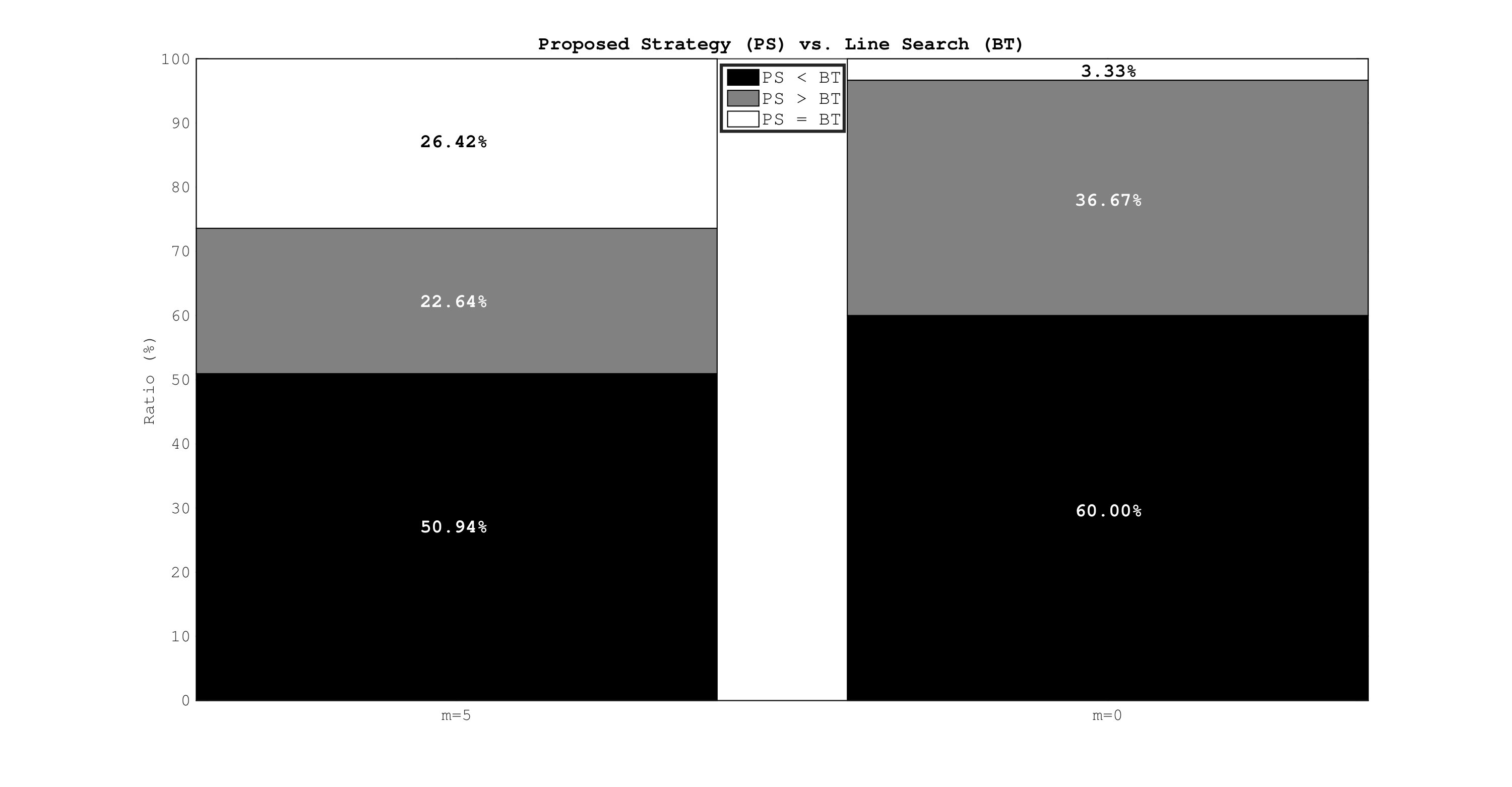 Figure 1
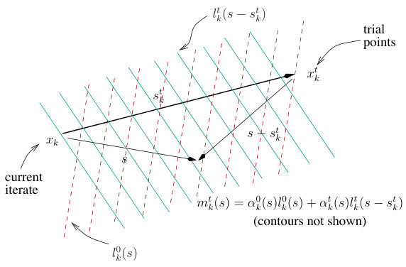 Figure 2
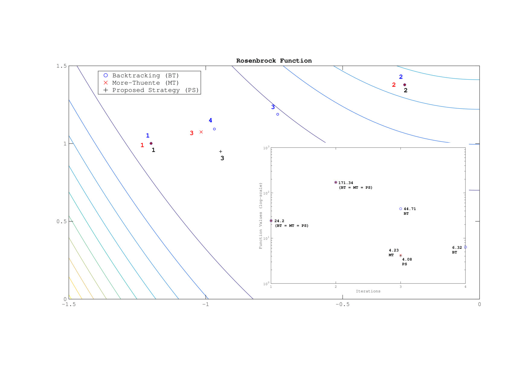 Figure 3
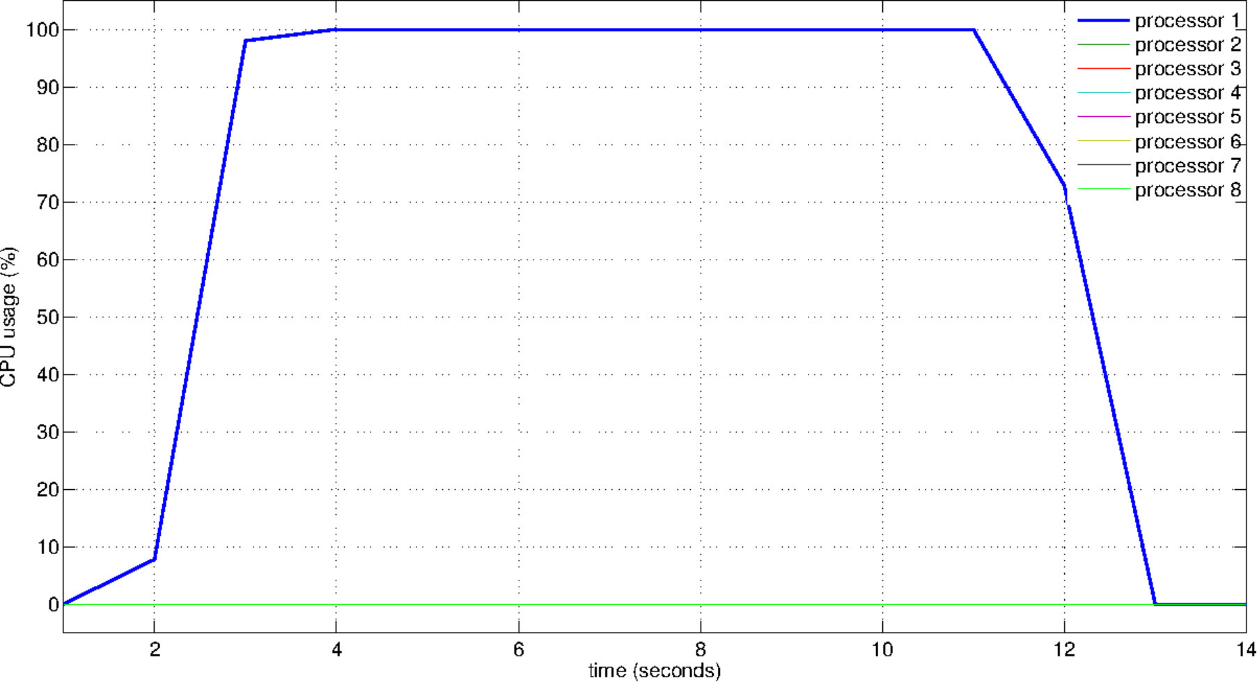 Figure 4
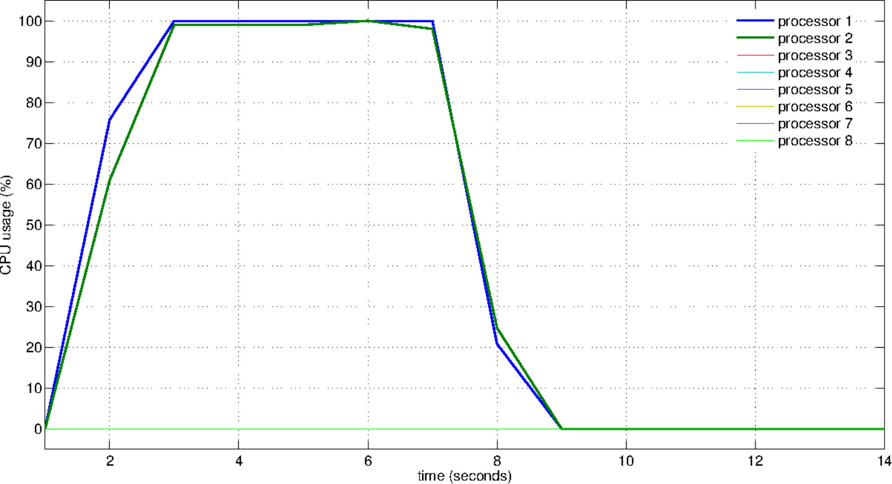 Figure 5
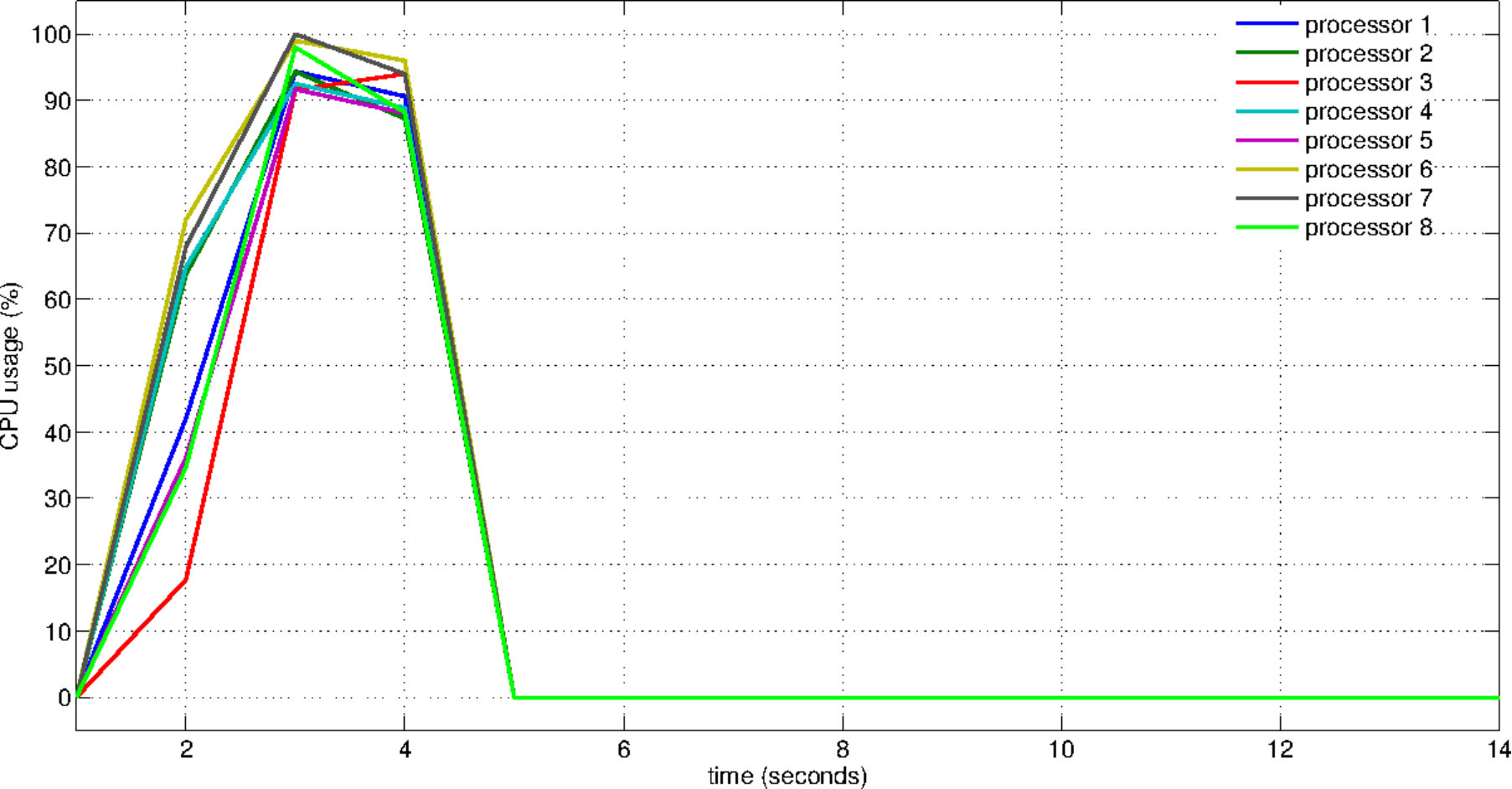 Figure 6
| Problem | ||||||
|---|---|---|---|---|---|---|
| 5M | 8.80 | 4.41 | 2.24 | 1.29 | 0.89 | |
| COSINE | 25M | 43.98 | 22.07 | 11.19 | 6.33 | 4.35 |
| 125M | 219.77 | 111.74 | 57.98 | 31.62 | 21.47 | |
| 5M | 25.19 | 12.57 | 6.49 | 4.08 | 2.88 | |
| NONCVXUN | 25M | 118.59 | 58.63 | 30.44 | 18.39 | 13.29 |
| 125M | 496.45 | 249.43 | 127.38 | 75.43 | 55.07 | |
| 5M | 45.93 | 22.69 | 11.89 | 7.91 | 6.11 | |
| ROSENBR | 25M | 219.52 | 111.16 | 57.02 | 35.74 | 28.31 |
| 125M | 1113.83 | 554.07 | 283.83 | 178.41 | 140.60 |
Peer Reviews
No public reviews on file for this paper yet. If you reviewed it on a platform where reviews are public (OpenReview, ICLR, NeurIPS, ICML), you can paste yours below so the community can read it here.
Videos
No videos yet. Explain this paper in a talk, walkthrough, or lecture? Add one.
An Alternative Globalization Strategy for Unconstrained Optimization
@addressi
@addressii
@addressiii
@addressiv
@addressv
Abstract
We propose a new globalization strategy that can be used in unconstrained optimization algorithms to support rapid convergence from remote starting points. Our approach is based on using multiple points at each iteration to build a representative model of the objective function. Using the new information gathered from those multiple points, a local step is gradually improved by updating its direction as well as its length. We give a global convergence result and also provide parallel implementation details accompanied with a numerical study. Our numerical study shows that the proposed algorithm is a promising alternative as a globalization strategy.
1 Introduction.
In unconstrained optimization, frequently used algorithms, like quasi-Newton or trust-region methods, need to involve mechanisms that ensure convergence to local solutions from remote starting points. Roughly speaking, these globalization strategies guarantee that the improvement obtained by the algorithm is comparable to the improvement obtained with a gradient step [NW06].
In this paper we present a new globalization strategy that can be used in unconstrained optimization methods for solving problems of the form
[TABLE]
where is a first order differentiable function. Conventional methods for solving this problem mostly use local approximations that are very powerful once the algorithm arrives at the close proximity of a stationary point. The main idea behind the proposed strategy is based on using additional information collected from multiple points to construct an adaptive approximation of the function in (1). In particular, we update our approximate model constructed around the current iterate and a sequence of trial points. Our objective is to come up with a better local model than the one obtained by the current iterate only. We observe that the collection of this additional information has a profound effect on the performance of the method as well. Before moving to the next iterate, the step is improved by updating its direction as well as its length simultaneously. This step computation involves only the inner products of vectors. Therefore, each iteration of the algorithm is amenable to a parallel implementation. Though acquiring the additional information from multiple points may add an extra burden on the algorithm, this burden can be alleviated by using the readily available parallel processors. Furthermore, our numerical experiments demonstrate that the additional computations at each step may reduce the total number of iterations, since we learn more about the function structure.
Parallel execution of linear algebra operations is common in the parallel optimization literature; generally in designing parallel implementations of existing methods. Among the earliest work is [BRS88], where parallelization of linear algebra steps and function evaluations in the BFGS method is discussed. Around the same time, [NS89] propose to use truncated-Newton methods combined with computation of the search direction via block iterative methods. In particular, they focus on the block conjugate-direction method. By using block iterative methods, they parallelize some steps of the algorithm, in particular, the linear algebra operations. For extensive reviews of the topic, we refer to [Zen89, MTK03, DW03].
The use of multiple trial points or directions is also a recurring idea in the field of parallel nonlinear optimization. However, unlike our case, these mostly depend on concurrent information collection / generation. [Pat84] proposes an algorithm, which is based on evaluating multiple points in parallel to determine the next iterate. In the parallel line search implementation of [PFZ98], multiple step sizes are tried in parallel. [vL85] discusses three parallel quasi-Newton algorithms that are also based on considering multiple directions to extend the rank-one updates. To solve the original problem by solving a series of independent subproblems, [Han86] suggests using conjugate subspaces for quasi-Newton updates. Thus, the resulting method can be applied in a parallel computing environment.
The rest of this paper is organized as follows. In Section 2, we discuss the derivation and the theoretical properties of the proposed strategy. In Section 3, the success of the main idea of the method is numerically tested, and its parallel implementation is discussed in Section 4. Conlusion of the study is presented in Section 5.
2 Proposed Globalization Strategy.
At the core of the proposed strategy lies an extended model function, which is constructed by using two linear models at two reference points. The first of these points is the current iterate and the second one is a trial point. When one of these trials leads to a successful step, then the algorithm moves to a new iterate. To make our discussion more concrete, we start by describing an iteration of the algorithm.
Let and denote the current iterate and the step of the algorithm, respectively. Then, the next iterate becomes . These are the outer iterations. The vector is obtained by executing a series of inner iterations and computing trial steps , . We can further simplify our exposition by defining
[TABLE]
The trial step is accepted as new , if it provides sufficient decrease in the sense
[TABLE]
This is nothing but the well-known Armijo condition [NW06].
Up to this point, the algorithm behaves like a typical unconstrained minimization procedure. However, to come up with the proposed globalization strategy, we design a new subprocedure for computing the trial steps, . The inner step computation is done by solving a subproblem that consists of an extended model function updated at every inner iteration and a constraint restricting the length of the steps. The extended model function is an approximation to the objective function, . It is constructed by using the information gathered around the region bordered by and . Actually, the extended model function is a combination of the linear models of at and . That is,
[TABLE]
where
[TABLE]
This construction is illustrated in Figure 1. Note that both weights, and are functions of . We want to make sure that if is closer to , then the weight of the linear model around increases. Similarly, should increase as gets closer to . This is achieved by measuring the length of the projections of and on by
[TABLE]
respectively.
Next, we introduce a constraint to handle the possibly hard quadratic function as well as control the step length. Recall that our model function is constructed around the previous trial step by considering the area lying between and . Thus, we impose the constraint
[TABLE]
Clearly, this constraint controls not only the length of but also its deviation from the previous trial point . In addition, this choice of the constraint ensures that both weight functions and are in and they add up to
- Hence, our model function is the convex combination of the linear functions and . This observation is formally presented in Lemma 2.1 and its proof is given in Appendix A.
Lemma 2.1
If constraint (5) holds at inner iteration of iteration , then both and are nonnegative, and they satisfy .
We also make the following observations about the region defined by constraint (5). First, this region is never empty, since any step for is in the region. This implies in a sense that a backtracking operation on the previous trial step, would give a new feasible trial step, . Second, there are always feasible steps in the steepest descent direction whenever holds. That is, the steps are feasible for . Thus, as long as the first trial step, is gradient related, each feasible region constructed around a subsequent trial step involves a feasible point that is also gradient related.
Algorithm 1 gives the outline of the proposed method. The stopping condition is the usual check whether the current iterate, is a stationary point. We start the inner iterations by computing the first trial step, . We shall elaborate on how to select this initial trial step in Section 4. As long as the trial steps , are not acceptable, we carry on with constructing and minimizing the model functions. Once an acceptable step is obtained by the inner iteration, we evaluate the next iterate and continue with solving the overall problem.
In Algorithm 1, the crucial part is solving subproblem (6), which has a quadratic objective function and a quadratic constraint. After some derivation, the objective function of this subproblem simplifies to
[TABLE]
where
[TABLE]
and
[TABLE]
The Hessian of this quadratic objective function is the rank-one matrix . Its only nonzero eigenvalue is , and the eigenvectors corresponding to this eigenvalue are and . Furthermore, its eigenvectors corresponding to the zero eigenvalues are perpendicular to . Let us note at this point that the gradient of the model is given by
[TABLE]
2.1 Convex Objective Function.
Before considering the general case, we discuss in this section how subproblem (6) can be solved when the objective function is convex. We shall soon observe that it is not straightforward to obtain trial steps that yield sufficient descent with this initial design. Thus, we will propose modifications over this first attempt in Section 2.2 to guarantee convergence. However, we still present here our observations with the convex case as it constitutes the basis of our approach for general functions given in the next section.
We first check whether the subproblem always provides a nonzero step at every inner iteration. It turns out that if the most recent trial step, is gradient related, then the next trial step, cannot be the zero vector. Furthermore, if the objective function value of the recent trial step is strictly greater than the current objective function value, then the optimal solution of the subproblem is in the interior of the region defined by the constraint (5). Lemma 2.2 summarizes this discussion. The proof of this lemma is given in Appendix A.
Lemma 2.2
Let be a convex function and consider the inner iteration of iteration with . If , then and
[TABLE]
If we additionally have , then .
Note that we require condition hold for all trial steps to guarantee nonzero trial steps. So, a convergence argument for the proposed algorithm is not clear unless it ensures this condition. We shall visit this issue later in this section.
We next show how subproblem (6) can be solved, if the conditions given in Lemma 2.2 hold. This subproblem can be rewritten as
[TABLE]
Note that this is a convex program as by the convexity assumption on in this section. Let denote the optimal solution of the above problem and be the Lagrange multiplier corresponding to the constraint. The Karush-Kuhn-Tucker optimality conditions imply
[TABLE]
Simplifying (8) leads to
[TABLE]
where
[TABLE]
[TABLE]
with
[TABLE]
Consider first the case when . Then, using Lemma 2.2, we have . When , the optimal solution is at the boundary of the constraint. If we now use (10) with (9), then after some derivation we obtain
[TABLE]
where is a sixth order polynomial function of (see the online supplement111http://people.sabanciuniv.edu/sibirbil/glob_strat/OnlineSupplement.pdf for the details). Thus, the subproblem can be solved by computing the roots of this polynomial.
In fact, it is not hard to show that if the inner iteration step satisfies for some matrix , then at the next inner iteration we have However, it is not possible to guarantee that the matrix will be positive definite given is. That is because the gradient of the model function is given as the conical combination of and . First of all, the model gradient can be zero for at a point with . Also, when the deviation of the objective function from linearity is relatively large, then the model gradient can point a backward direction; i.e. the reverse direction of . Since the constraint of the model does not allow such a backward step, this can cause to be zero. Moreover, the model gradient is scaled with a matrix, and the scaled step adds a third component along to the linear combination whose coefficient is not necessarily positive. So, the resulting might not satisfy even if does.
2.2 General Objective Function.
Using our observations on the convex case, we next concentrate on a construction where the model function has the same gradient value at as the original objective function, . Then, we also add a regularization term so that the subproblem can be made convex even if is not.
We start by relaxing the constraint (5) and moving it to the objective function. That is
[TABLE]
We choose
[TABLE]
so that . Observe that the above choice of can be negative (for nonconvex), in which case the constraint operates the reverse way; i.e. it tries to keep away from . Since that causes us to loose our control on the size of , we add a regularization term and the subproblem becomes
[TABLE]
After simplifying the objective function, we obtain our new subproblem for the general case
[TABLE]
where
[TABLE]
Note that the model function (11) is always convex provided that the regularization parameter is chosen sufficiently large. Beyond the convexity of , we want to guarantee for some that the steplength condition
[TABLE]
holds. Suppose is such a step and it is the optimal solution for problem (11) with a convex objective function. Then, the first order optimality condition implies
[TABLE]
where
[TABLE]
Thus, we obtain
[TABLE]
where denotes the smallest eigenvalue of its matrix parameter. It is not difficult to see that is an eigenvalue of with multiplicity , and the remaining two eigenvalues are the extreme eigenvalues of given by
[TABLE]
where denotes the largest eigenvalue of its matrix parameter.
To obtain a convex model, we need
[TABLE]
On the other hand, the steplength condition (12) requires
[TABLE]
Since the latter bound is larger, using relation (15) for choosing provides the convexity requirement and satisfies the steplength condition. That is
[TABLE]
Our last step is to state the minimizer of (11) with selected and values. Following similar steps as in Section 2.1, after some derivation we obtain
[TABLE]
where
[TABLE]
[TABLE]
with
[TABLE]
and
[TABLE]
It is important to observe that the solution of the subproblem does not require storing any matrices and the main computational burden is only due to inner products, which could be done in parallel (see Section 4).
When it comes to the convergence of the proposed algorithm, we are saved basically by keeping the directions of its steps gradient related. However, we could not directly refer to the existing convergence results, since the directions in our algorithm change during inner iterations and the steplength is not computed by using a one dimensional function. In the following convergence note, we only assume additionally that the objective function is bounded below and its gradient is Lipschitz continuous with parameter .
Lemma 2.3
Suppose that the first trial step satisfies and for some . Then, at any iteration , the optimal solution in (16) becomes an acceptable step satisfying (2) in finite number of inner iterations at a nonstationary point .
Proof.
Consider any iteration . Since is obtained by (13), the steps computed at each inner iteration satisfy , for . Note for that by the choice of and the relation (14). We have
[TABLE]
Using (12), we have . Then,
[TABLE]
Therefore, we obtain
[TABLE]
Suppose that the acceptance criterion (2) is never satisfied as . Then,
[TABLE]
This implies
[TABLE]
Next the desired inequality is obtained by
[TABLE]
Since , the right hand side of the last inequality increases without a bound as . This gives a contradiction as is bounded. So, an acceptable should be obtained in finite number of inner iterations. ∎
Note that the conditions on the initial step length, in Lemma 2.3 are simply satisfied, if we choose for any . This implies .
Theorem 2.1
Let be the sequence of iterates generated by Algorithm 2 and satisfy the requirements in Lemma 2.3. Then, any limit point of is a stationary point of the objective function .
Proof.
By Lemma 2.3, for any , (2) is satisfied after a finite number of inner iterations, say . Also, note that relation (13) implies with the same as in (18). We will now derive a lower bound for :
[TABLE]
So,
[TABLE]
Recall that for the accepted step of iteration we have . Clearly, is bounded away from zero as is finite. Consider now any subsequence of with indices such that
[TABLE]
Then, for any with we have
[TABLE]
Since converges to , the continuity of implies that as . Therefore as . Thus, we obtain by (19) since is bounded away from zero. ∎
2.3 Relationship with Quasi-Newton Updates.
Observing the formula in (13), we next question the relationship between the step computation of the proposed algorithm and the quasi-Newton updates, in particular the DFP formula [NW06]. The key to understanding this relationship is to treat the current iterate as the previous iterate, whereas our trial step becomes the next iterate in standard quasi-Newton updates.
Let denote the quasi-Newton approximation to the Hessian at iterate . Then, the infamous DFP formula yields the new approximation to the Hessian in the next iterate as
[TABLE]
where and . We first substitute for and for in the above equation. Then, by setting
[TABLE]
we obtain
[TABLE]
Let us now denote the Hessian of the objective our model function given in relation (11) by . Then, we have
[TABLE]
Next we plug in the value of from (17) and obtain
[TABLE]
The last term above, in a sense, serves the purpose of obtaining a positive definite matrix. Thus, the objective function becomes convex. Looking at our approach from the quasi-Newton approximation point of view, we again confirm that the additional information collected from the trial iterate is used to come up with a better model around the current iterate . Our derivation above also shows that the construction of the model function from one inner iteration to the next is completely independent.
3 Practical Performance.
In this section, we shall conduct a numerical study to demonstrate the novel features of the proposed globalization strategy. We have compiled a set of unconstrained optimization problems from the well-known CUTEst collection [GOL04]. We have also embedded the proposed strategy (PS) into the L-BFGS package [Oka10] as a new globalization alternative to the existing two line search routines; backtracking (BT) and More-Thuente line search (MT).
First, let us give a two-dimensional example to illustrate how the proposed strategy can be beneficial. Figure 2 shows the contours of the Rosenbrock function. The inner iterates of PS are denoted by markers, the inner iterates of BT are denoted by markers, and the inner iterates of MT are denoted by markers. All three globalization strategies start from the same initial point. The numbers next to the trial points denote the inner iterations. The corresponding objective function values are given in the subplot at the southeast corner of the figure.
Figure 2 illustrates the main point of the proposed strategy: PS can change the direction of the trial step as well as its length. It is important to note that PS is not a trust-region method because it builds a new model function by using the current trial step for computing the next trial step. However, in a trust-region method the model function is not updated within the same iteration and the current trial step does not contribute to the computation of the next trial step. For this particular two-dimensional problem, PS performs better than the other two globalization strategies as it attains the lowest objective function value after three inner iterations.
Next, we test the effect of the direction updates introduced by the proposed strategy. We solve the CUTEst problems by employing the backtracking line search with Wolfe conditions using the default reduction factor of 0.5 given in the L-BFGS package. For the proposed strategy, we also set the parameter to 0.5. Therefore, the new strategy requires the same amount of steplength decrease (but it may additionally alter the search direction). In our tests, we start with both the L-BFGS step with memory set to 5 () and the gradient step (). The maximum number of iterations is set to 500 for the L-BFGS step, and to 1,000 for the gradient step. The comparison is carried out for those problems, where both methods obtained the same local solution (which is assessed by comparing the objective function values and the first two components of the solution vectors). The results are reported for 30 problems when , and for 63 problems when .
Figure 3 summarizes our observations. We compare two strategies in terms of the total number of function evaluations required to solve the problems. When , solving of the problems required less number of function evaluations than the line search. The same figure becomes when , and solving of the problems took exactly the same number of iterations with both strategies. Overall, these results show that the direction updates of the new strategy can indeed provide improvements.
4 Parallel Implementation.
In this section, we will provide an outline of the subproblem solution operations while we discuss their parallel execution. Then, we conduct some numerical experiments to illustrate the parallel performance of the proposed algorithm.
As relation (16) shows, the basic trial step at inner iteration is in the subspace spanned by , , and the previous trial step . We should also emphasize that the computation of requires just a few floating point operations, once the necessary inner products are completed. In particular, the computation of (16) requires the following inner products.
[TABLE]
Once the scalar values , are available, the multipliers , , in (16) can be computed in a total of 32 floating point operations as follows:
[TABLE]
Clearly, the total cost of synchronization operations is negligible. Thus, the parallel execution of the above inner products determine the parallel performance as well as the two remaining components of the algorithm: the computation of initial trial step and function/gradient evaluations. We require that is computed without introducing too much sequential work to the overall algorithm, and satisfy the conditions in Section 2. A simple choice could be the gradient step, which we also preferred in our own implementation.
The parallel implementation given in Algorithm 2 is considered for a shared memory environment with physical cores (threads). Note that the parallel implementation of function/gradient computations is clearly problem dependent. However –at least partial– separability is likely to occur for large-scale problems. This issue, we assume, is taken care of by the user.
We coded the algorithm in C using OpenMP. We have selected three test problems from the CUTEst collection [GOL04], whose dimensions can be varied to obtain small- to large-scale problems, namely COSINE, NONCVXUN, and ROSENBR. The objective functions of the problems, and the initial points used in our tests are as follows:
[TABLE]
where denotes the th component of point and is the initial point. We note that the function and gradient evaluations of all three test problems are in the order of . So, function evaluations are not dominant to the computations of the new strategy. Moreover, the evaluations of all three functions can be done in parallel with one synchronization in computing the objective function value.
To test the parallelization performance of the algorithm, we set the dimension of the problems to million, million and million, and solve each of the resulting instances for various values of the total number of threads, . We run the algorithm by setting , and the step acceptability is checked using condition (2) with . We set both the maximum number of inner iterations and the maximum number of outer iterations to . If the algorithm cannot reach a solution with the desired accuracy
[TABLE]
then we report the clock time elapsed until the maximum number of outer iterations is reached. We summarize these results in Table 1 We observe that the speed-up is close to linear for up to 8 cores. Since there is no data reuse, if we further increase the number of cores, the main memory bandwidth becomes the bottleneck. This is a common issue when memory-bounded computations, like inner product evaluations, are parallelized.
Finally, we consider the load balance issue. To observe the usage of capacity and the workload distribution, we plot the CPU usage during the solution of 1M-dimensional instance of the problem COSINE (see Figure 4). The plots are obtained by recording the CPU usage information per second via the mpstat command-line tool (see Linux manual pages). Figure 4(a) reveals the idle resources when the program runs sequentially. In fact, during the sequential run, the average resource usage stays at a level of . This value is computed by taking the average usage of eight cores. When eight threads are used, this average raises up to . Figure 4(c) shows the usage of all available resources as well as the distribution of the workload.
5 Conclusion and Future Research.
The current study is a part of our research efforts that aim at harnessing parallel processing power for solving optimization problems. Our main motivation here was to present the design process that we went through to come up with an alternate globalization strategy for unconstrained optimization that can be implemented on a shared memory parallel environment.
The proposed algorithm works with a model function and considers its optimization over an elliptical region. However, it does not employ a conventional trust-region approach. Nor does it match with any one of the well-known quasi-Newton updates. The basic idea is to use multiple trial points for learning the function structure until a good point is obtained. These trials constitute the inner iterations. Fortunately, all these computations of the algorithm are domain-separable with two synchronization points at each inner iteration.
Our numerical experience verifies that the direction updates of the resulting algorithm can reduce the total number of function evaluations required, and it is scalable to a degree allowed by the inner iterations with a balanced distribution of the workload among parallel processors. Like any parallel optimization method, the parallel performance of the proposed algorithm can be compromised if function evaluations are computationally intensive and unfit for parallelization.
We only solved a set of examples with our algorithm. It is yet to be seen whether the algorithm is apt for solving other large-scale problems, especially those ones arising in different applications. In our implementation, we chose the initial trial point simply by using the negative gradient step. One may try to integrate other, potentially more powerful but still parallelizable, steps to the algorithm. An example could be using a truncated Newton step; perhaps computed by a few iterations of the conjugate gradient on the initial quadratic model. Then switching to the globalization strategy, as described here, could adjust the direction and the length of the initial step. Finally, our observations on the relationship of the new strategy with the quasi-Newton update formulas can be studied further in future research.
A Omitted Proofs.
Lemma 2.1* If constraint (5) holds at inner iteration of iteration , then both and are nonnegative, and they satisfy . *
Proof.
We have
[TABLE]
Since constraint (5) implies , we obtain
[TABLE]
The result follows from the definitions of and . ∎
Lemma 2.2* Let be a convex function and consider the inner iteration of iteration with . If , then and*
[TABLE]
*If we additionally have , then . *
Proof.
By using relation (7), we have
[TABLE]
Since is a convex function, we know that . If , then because is not a stationary point. Now, consider the case , and suppose for contradiction that . Then,
[TABLE]
Multiplying both sides with , we obtain
[TABLE]
Since , we obtain a contradiction and hence . This shows that . Note that
[TABLE]
This implies that is a descent direction for at . Then, it is easy to solve the one-dimensional convex optimization problem to obtain
[TABLE]
Again by using relation (7), we have
[TABLE]
which gives
[TABLE]
If along with , then
[TABLE]
holds. Therefore, we have , which implies that is a descent direction for at . In this case, the minimizer along should be in the interior. Thus, . ∎
The reference list from the paper itself. Each links out to its DOI / PubMed record.
- 1[BRS 88] R.H. Byrd, Schnabel R.B., and G.A. Shultz. Parallel quasi-Newton methods for unconstrained optimization. Mathematical Programming , 42(1):273–306, 1988.
- 2[DW 03] Jr. J.E. Dennis and Z. Wu. Parallel continuous optimization. In J. Dongarra, I. Foster, G. Fox, W. Gropp, K. Kennedy, L. Torczon, and A. White, editors, Sourcebook of parallel computing , pages 649–670. Morgan Kaufmann Publishers Inc., San Francisco, CA, USA, 2003.
- 3[GOL 04] N. I. M. Gould, D. Orban, and Toint P. L. CUT Er (and Sif Dec), a constrained and unconstrained testing environment, revisited. Technical Report TR/PA/01/04, CERFACS, 2004.
- 4[Han 86] S.-P. Han. Optimization by updated conjugate subspaces. In D. Griffiths and G. Watson, editors, Numerical Analysis , pages 82–97. Longman Scientific and Technical, 1986.
- 5[MTK 03] A. Migdalas, G. Toraldo, and V. Kumar. Nonlinear optimization and parallel computing. Parallel Computing , 29:375–391, 2003.
- 6[NS 89] S.G. Nash and A. Sofer. Block truncated-Newton methods for parallel optimization. Mathematical Programming , 45:529–546, 1989.
- 7[NW 06] J. Nocedal and S. J. Wright. Numerical Optimization . Springer, 2006.
- 8[Oka 10] N. Okazaki. C port of the L-BFGS method written by jorge nocedal, 2010. http://www.chokkan.org/software/liblbfgs/ .