This paper introduces a new class of graph transformations based on parameters and derives the Laplacian spectra of these transformed graphs for regular graphs, linking them to the original spectra and graph parameters.
Contribution
It provides a complete description of the Laplacian spectra of (x,y,z)-transformations of regular graphs, connecting the spectra to original graph properties.
Findings
01
Laplacian polynomial of G(x,y,z) depends on |V|, r, and G's Laplacian spectrum.
02
Explicit formulas for spectra of transformed graphs.
03
Applicable to regular graphs with various parameter choices.
Abstract
For any given graph G = (V,E) we define in a certain way a new graph G(x,y,z) with the vertex set V\cup E depending on parameters x,y,z from {0,1, +, -} and call graph G(x,y,z) the (x,y,z)-transformation of G. It turns out that if G is an r-regular graph, then the Laplacian polynomial of G(x,y,z) is a function of |V|, r, and the Laplacian spectrum of G. We give a complete description of this function.
A(G^{0++})=\left(\begin{array}[]{cc}0&\quad Q\\[4.30554pt]
Q^{\top}&\quad A(G^{l})\end{array}\right)\hbox{\ and \ }D(G^{0++})=\left(\begin{array}[]{cc}rI_{n}&\quad 0\\[4.30554pt]
0&\quad 2rI_{m}\end{array}\right).
A(G^{0++})=\left(\begin{array}[]{cc}0&\quad Q\\[4.30554pt]
Q^{\top}&\quad A(G^{l})\end{array}\right)\hbox{\ and \ }D(G^{0++})=\left(\begin{array}[]{cc}rI_{n}&\quad 0\\[4.30554pt]
0&\quad 2rI_{m}\end{array}\right).
L(λ,G0++)
L(λ,G0++)
L(λ,G0++)
L(λ,G0++)
21(r+2+λi±λi2−2rλi+r2+4r+4),i=1,2,⋯,n.
21(r+2+λi±λi2−2rλi+r2+4r+4),i=1,2,⋯,n.
t(G0++)=m+nn2m−n(r+1)m−1(r+2)t(G).
t(G0++)=m+nn2m−n(r+1)m−1(r+2)t(G).
Peer Reviews
No public reviews on file for this paper yet. If you reviewed it on a platform where reviews are public (OpenReview, ICLR, NeurIPS, ICML), you can paste yours below so the community can read it here.
Videos
No videos yet. Explain this paper in a talk, walkthrough, or lecture? Add one.
Full text
Laplacian Spectra of Regular Graph Transformations
††thanks: Aiping Deng and Juan Meng are supported in part by the Fundamental Research Funds for the Central Universities of China 11D10902 and
11D10913.
Aiping Denga111Corresponding author.
Email: [email protected]. Tel: 86-21-67792089-568. Fax: 86-21-67792311 ,
Alexander Kelmansb,c, Juan Menga
a*Department of Applied Mathematics, Donghua University, 201620 Shanghai, China *
b*Department of Mathematics, University of Puerto Rico, San Juan, PR, United States
cDepartment of Mathematics, Rutgers University, New Brunswick, NJ, United States*
Abstract
Given a graph G with vertex set V(G)=V and edge set E(G)=E, let Gl be the line graph and Gc the complement of G.
Let G0 be the graph with V(G0)=V and with no edges, G1 the complete graph with the vertex set V, G+=G and
G−=Gc.
Let B(G) (Bc(G)) be the graph with the vertex set V∪E and
such that (v,e) is an edge in
B(G) (resp., in Bc(G))
if and only if v∈V, e∈E and vertex v is incident (resp., not incident) to edge e in G. Given x,y,z∈{0,1,+,−},
the xyz-transformation Gxyz ofG
is the graph with the vertex set V(Gxyz)=V∪E and the edge set E(Gxyz)=E(Gx)∪E((Gl)y)∪E(W), where
W=B(G) if z=+,
W=Bc(G)
if z=−, W is the graph with
V(W)=V∪E and with no edges if z=0, and
W is the complete bipartite graph with parts V and E if z=1.
In this paper we obtain the Laplacian characteristic polynomials and some other Laplacian parameters of
every xyz-transformation of an r-regular graph G in terms of ∣V∣, r, and the Laplacian spectrum
of G.
The graphs in this paper are simple and undirected.
All notions on graphs and matrices that are used but not defined here can be found in
[1, 5, 6, 8, 22].
Let G denote the set of simple undirected graphs.
Various important results in graph theory have been obtained by considering some functions
F:G→G
or Fs:G1×…×Gs→G called
operations or transformations
(here each Gi=G) and
by establishing how these operations affect certain properties or parameters of graphs.
The complement, the k-th power of a graph, and the line graph are well known examples of such operations.
The Bondy-Chvátal and Ryzác̆ek closers of graphs are very useful operations in graph Hamiltonicity theory
[1].
(Strengthenings and extensions of the Ryzác̆ek result are given in [9]).
Some graph operations introduced by A. Kelmans
(see, in particular, [10, 13]) turn out to be
monotone with respect to various partial order relations on the set of graphs.
For that reason these operations
turned out to be very useful in obtaining
non-trivial results on graphs of given size with various extreme properties (with the maximum number of spanning trees and some other Laplacian parameters of graphs, with the maximum reliability of graphs having randomly deleted edges, etc.),
see, for example, [11, 12].
The operation of voltage lifting on a base graph introduced by Gross and Tucker can be generalized to digraphs
[4, 7].
Using this operation one can obtain the derived covering (di)graph and deduce the relationship between the adjacency characteristic polynomials of the base (di)graph and its derived covering (di)graph [4, 3, 19, 25].
In this paper we consider certain graph operations
depending on parameters x,y,z∈{0,1,+,−}.
These operations induce functions Txyz:G→G. We put Txyz(G)=Gxyz and call
Gxyz the xyz-transformation of G.
We describe for all x,y,z∈{0,1,+,−}
the Laplacian characteristic polynomials and some other Laplacian parameters of
xyz-transformations of an r-regular graph G.
This descriptions revealed the following fact interesting in itself: if G is r-regular, then
the Laplacian spectrum of Gxyz is uniquely defined by ∣V(G)∣, r,
and the Laplacian spectrum of G; moreover, the Laplacian eigenvalues are the roots of a quadratic polynomial with the coefficients depending on ∣V(G)∣, r, and the Laplacian spectrum of G.
Furthermore, for (xyz)∈{(00+),(0++),(+0+)}
the number of spanning trees of Gxyz are uniquely defined by ∣V(G)∣, r, and the number of spanning trees of G (see Theorem 2.5 and Corollaries 3.5, 3.9, and 3.12 below).
The approach we have used to obtain all these formulas may also be useful in further research along this line. The results of this paper may be considered as a natural and useful extension of Section 2 “Operations on Graphs and the Resulting Spectra” in book [2].
The Reciprocity Theorem [16] (see also Theorem 2.6 below) provides for every graph G the relation between the Laplacian characteristic polynomial of G and its complement Gc. For that reason it is sufficient to describe the Laplacian characteristic polynomials of graph xyz-transformations up to
the graph operation of taking the complement.
In Section 2 we introduce main
notions, notation, simple observations, and some preliminaries.
In Section 3 we describe (up to the complementarity) the Laplacian characteristic polynomials of the transformations Gxyz with {x,y,z}∩{0,1}=∅.
In Section 4 we describe
the Laplacian characteristic polynomials of transformations Gxyz with {x,y,z}∩{0,1}=∅, i.e. with x,y,z∈{+,−}.
In Sections 5 we consider some transformations of cycles and show that different transformations of the same graph may be isomorphic. Section 6 contains some additional remarks.
In the Appendix we provide for all x,y,z∈{0,1,+,−} the list of formulas
for the Laplacian characteristic polynomials and the number of spanning trees of the (xyz)-transformations of an r-regular graph G in terms of r,
the number of vertices, the number of edges, and the Laplacian spectrum of G. This catalog may be pretty useful for further research in the spectrum graph theory.
2 Some notions, notation, and preliminaries
Let G=(V,E) be a graph with vertex set
V=V(G) and edge set
E=E(G). Let v(G)=∣V(G)∣ and e(G)=∣E(G)∣.
The degreed(v,G)of vertexv∈V is the number of vertices in G adjacent to v.
Let t(G) denote the number of spanning trees of G.
Given two graphs G and H, an isomorphism from G to H is a bijection α from V(G) to V(H) such that (u,v)∈E(G)⇔(α(u),α(v))∈E(H).
The complementGc of a graph G is the graph with vertex set V(Gc)=V(G) and (u,v)∈E(Gc)⇔(u,v)∈E(G) for any
u,v∈V(G) and u=v.
The line graphGl of a graph G is the graph
with vertex set E(G) and two vertices are adjacent in Gl if and
only if the corresponding edges in G are adjacent.
Graphs G and H are called isomorphic if there exists an isomorphism from G to H.
For a graph
G=(V,E), let
G0 be the graph with V(G0)=V and with no edges, G1 the complete graph with V(G1)=V,
G+=G, and G−=Gc.
Let B(G) (Bc(G)) be the graph with the vertex set V∪E and
such that (v,e) is an edge in
B(G) (resp., in Bc(G)) if and only if v∈V, e∈E, and vertex v is incident (resp., not incident) to edge e in G.
For example, in Figure 1,
G00+=B(G) and Bc(G) is obtained from
G01− by deleting the edge connecting two white vertices.
The graph transformations we are going to discuss are defined as follows.
Definition 2.1**.**
Given a graph G=(V,E) and three variables
x,y,z∈{0,1,+,−}, the xyz-transformation Gxyz ofG is the graph with the vertex set
V(Gxyz)=V∪E
and the edge set E(Gxyz)=E(Gx)∪E((Gl)y)∪E(W), where
W=B(G) if z=+, W=Bc(G) if z=−, W is the graph with V(W)=V∪E and with no edges if z=0, and
W is the complete bipartite graph with parts V and E if z=1.
Examples of xyz-transformations of a 3-vertex path are given in Figure 1.
Graphs G+++ and G00+ are called in [2] the total graph and the subdivision graph of G, respectively.
Let G be a graph with vertex set
V={v1,…,vn} and edge set
E={e1,…,em}.
The incidence matrixQ(G) of G is
the (V×E)-matrix {qij}, where
qij=1 if vertex vi is incident to edge ej and
qij=0, otherwise.
Let A(G) be the (V×V)-matrix {aij}, where
aij=1 if (vi,vj)∈E and aij=0, otherwise.
Let D(G) be the (diagonal) (V×V)-matrix
{dij}, where dii=d(vi,G) and dij=0 for i=j.
The matrices A(G), D(G) and L(G)=D(G)−A(G) are called
the adjacency matrix, the degree matrix, and the Laplacian matrix of G, respectively.
The adjacency polynomial,
the adjacency spectrum and the
adjacency eigenvalues of G are
the characteristic polynomial
A(α,G)=det(αI−A(G)),
the spectrum, and the eigenvalues
of A(G), respectively.
Similarly, the
Laplacian polynomial, the
Laplacian spectrum and the
Laplacian eigenvalues of G are
the characteristic polynomial
L(λ,G)=det(λI−L(G)),
the spectrum, and
the eigenvalues of L(G), respectively.
Let In be the identity (n×n)-matrix and
Jmn the all-ones m×n-matrix.
Since A(G) and L(G) are symmetric matrices,
their eigenvalues are real numbers.
It is easy to see that each row sum of L(G) is equal to zero and that
L(G) is a symmetric positive semi-definite matrix
[2, 15]. Therefore all eigenvalues λi(G) of L(G)
are real non-negative numbers and one of them is equal to zero; we order them in the descendant order:
[TABLE]
The set Sp(G)={λ1(G),…,λn(G)} is called the Laplacian spectrum of G.
Some graph properties
of the transformations Gxyz with x,y,z∈{+,−} have been discussed and obtained in [17, 23, 24].
For a regular graph G, the adjacency characteristic polynomials and the adjacency spectrum of G00+,
G+0+, G0++ and the total graph G+++ are given in [2] (pages 63 and 64).
The adjacency characteristic polynomials and the adjacency spectrum of the other seven Gxyz with x,y,z∈{+,−} are obtained in
[26].
The definition of xyz-transformation can be easily extended to digraphs, which is also a generalization of the digraph transformations defined by Liu and Meng [18]. Zhang, Lin, and Meng have described
the adjacency characteristic polynomials of D00+,D+0+,D0++ and the total digraph D+++ for any digraph D [27]. The adjacency characteristic polynomials of other Dxyz of a regular digraph D with x,y,z∈{+,−} are obtained in [18].
Very few results are known for the Laplacian spectra of transformations.
In 1967 A. Kelmans published the following results
on the Laplacian polynomial of G0++, G0+0,
G00+, and Gl for a regular graph G.
These results are included in the survey papers
[20] (Theorem 3.8) and [21] (Theorem 1.4.2) with an error, namely,
graph G0++ is mistakenly called the total graph of
G.
Theorem 2.2**.**
[15]*
Let G be an r-regular graph with n vertices and m edges. Then*
[TABLE]
Theorem 2.3**.**
[15]*
Let G be an r-regular graph with n vertices and m
edges. Then*
[TABLE]
Theorem 2.4**.**
[15]*
Let G be an r-regular graph with n vertices and m edges. Then*
[TABLE]
Since nt(G)=(−1)n−1λ−1L(λ,G)∣λ=0, where n=v(G) [16],
we have from Theorems 2.2, 2.3, and 2.4:
Theorem 2.5**.**
[15]*
Let G be an r-regular graph with n vertices and m
edges. Then*
[TABLE]
[TABLE]
and
[TABLE]
A set A of graphs is closed under complementarity if for every graph in A its complement is also in A.
Given a graph G and S⊆{0,1,+,−}, let
F(G,S) denote the set of graphs Gxyz such that x,y,z∈S.
If F(G,S) is closed under complementarity, then in order to find the Laplacian polynomial for the graphs in
F(G,S), it is sufficient to find the solutions for a “half” of graphs in F(G,S) and to obtain the solutions for the graphs of the other “half” using the Reciprocity Theorem2.6 [16].
It is easy to see that F(G,{+,−}) and F(G,{0,1,+,−}) (and therefore F(G,{0,1,+,−}∖{+,−})) are closed under complementarity.
Hence the Reciprocity Theorem below can be used for these
classes of transformations.
The following two useful and very well known lemmas are obvious.
Lemma 2.8**.**
*Given a graph G with m edges, let
Gl be the line graph of G and Q the incidence matrix of G. Then
(a1)QQ⊤=D(G)+A(G) and
(a2)Q⊤Q=2Im+A(Gl).*
Lemma 2.9**.**
*Let G be an r-regular graph with n vertices and m edges and let A and Q be the adjacency and the incidence matrix of G, respectively.
Let k be a positive integer. Then
(a1)Q⊤Jnk=2Jmk,
(a2)QJmk=rJnk,
(a3)JkmQ⊤=rJkn,
(a4)JknQ=2Jkm,
(a5)JknA=rJkn, and
(a6)AJnk=rJnk.*
Lemma 2.10**.**
*Let G be an r-regular graph with n vertices, A(G)=A, and
λ1≥λ2≥⋯≥λn=0 the list of the Laplacian eigenvalues of G.
Let P(x,y) be a polynomial with two variables and real coefficients.
Then matrix P(A,Jnn) has the eigenvalues σn=P(r,n) and σi=P(r−λi,0) for
i=1,2,⋯,n−1.*
Proof.
Since the Laplacian matrix L=L(G) is symmetric and real, there is a list B={X1,X2,⋯,Xn} of mutually orthogonal eigenvectors of L, where Xi corresponds to λi and Xn=Jn1. Since
A=rIn−L, clearly AXi=(r−λi)Xi for each i. Since B is an orthogonal basis,
JnnXi=0 for each i=n.
Clearly, JnnJn1=nJn1 and
Jnn2=nJnn. By Lemma 2.9,
AJnn=JnnA=rJnn.
Therefore, P(A,Jnn)Xn=P(r,n)Xn and
P(A,Jnn)Xi=P(r−λi,0)Xi for each i=n.
□
The arguments in this proof are similar to those in
[14].
3 Laplacian spectra of Gxyz with
{x,y,z}∩{0,1}=∅
Given a graph G with n vertices and m edges, we always denote by A, D and Q, the adjacency matrix, the degree matrix and
the incidence matrix of G, respectively, and so if
G is an r-regular graph, then
D=rIn and 2m=rn.
We put λi(G)=λi, and so
λ1≥λ2≥⋯≥λn=0 is the list of the Laplacian eigenvalues of G.
3.1 Laplacian spectra of Gxyz with z=0
We start with the following simple observation.
Theorem 3.1**.**
Let G be a graph with n vertices and m edges and
let x,y∈{0,1,+,−}. Then
L(λ,Gxy0)=L(λ,Gx)L(λ,(Gl)y).
Since L(λ,G0)=λn, L(λ,G+)=L(λ,G) and L(λ,G1)=λ(λ−n)n−1,
we can calculate L(λ,Gxy0) for x,y∈{0,1,+,−} from
Theorems 2.3,
2.6 and 3.1.
Theorem 3.2**.**
*Let G be an r-regular graph with n vertices and m edges.
Then
(a1)L(λ,Gx00)=λmL(λ,Gx) and L(λ,Gx10)=λ(λ−m)m−1L(λ,Gx)
for x∈{0,1,+},
If G is an r-regular graph with n vertices and m edges, then G0++ has m−n Laplacian eigenvalues equal to 2r+2 and the following 2n Laplacian eigenvalues
[TABLE]
Corollary 3.12**.**
Let G be an r-regular graph with n vertices and m edges. Then
[TABLE]
Theorems 3.3 and 3.10 and Corollaries
3.5, 3.9, and 3.12
coincide with the corresponding Theorems 2.2, 2.4, and 2.5 by Kelmans.
The remaining situations when z=+ and
∣{x,y}∩{0,1}∣=1 can be considered similarly.
Here is the list of the Laplacian characteristic polynomials of Gxyz for these situations.
Theorem 3.13**.**
*Let G be an r-regular graph with n vertices and m edges. Then
Using the Reciprocity Theorem 2.6
it is easy to find from Theorems 3.2, 3.3,
3.6,
3.7, 3.10 and 3.13
the Laplacian characteristic polynomial of every Gxyz with {x,y}∩{0,1}=∅ and z∈{1,−} (see Appendix).
4 Laplacian spectra of Gxyz with
x,y,z∈{+,−}
In this section we will describe
the Laplacian characteristic polynomials and the Laplacian spectra of transformations Gxyz of an r-regular graph G for
x,y,z∈{+,−} in terms of the Laplacian spectrum of
G, r, v(G)=n, r (and e(G)=m=21rn).
Theorem 4.1**.**
Let G be an r-regular graph with n vertices and m edges.
Then
[TABLE]
Proof. The adjacency matrix and the degree matrix of
G+++ are
[TABLE]
Since L(G+++)=D(G+++)−A(G+++),
L(λ,G+++)=det(λIn−L(G+++)), and by Lemma 2.8(a2),
A(Gl)=Q⊤Q−2Im,
we have:
[TABLE]
Clearly, it is sufficient to prove our claim for
λ=2r+2.
Using Lemmas 2.7
we obtain:
[TABLE]
By Lemma 2.8(a1), QQ⊤=rIn+A. Therefore
L(λ,G+++)=(λ−2r−2)m−n×∣B∣, where
[TABLE]
Obviously, ∣B∣ equals the product of its eigenvalues.
By Lemma 2.10,
the eigenvalues of B are
σi=(λ−2r−2)((λ−2r)+r−λi)+(r+r−λi)((λ−2r−1)+r−λi)=(λ−r−λi)(λ−2−λi)−2r+λi
for i=1,2,…,n.
Let G be an r-regular graph with n vertices and m edges.
Then
[TABLE]
Proof. From the definition of G+−+, we have:
[TABLE]
For every z∈V(G+−+), d(z,G+−+)=2r if z∈V(G) and d(z,G+−+)=2+m−1−(2r−2)=m−2r+3 if
z∈E(G).
Therefore,
[TABLE]
Then L(λ,G+−+)=∣M∣, where
[TABLE]
By Lemma 2.9(a4), JmnQ=2Jmm.
Hence multiplying the first row of the block matrix M by
Q⊤−21Jmn and adding the result to the second row of M, we obtain a new matrix
[TABLE]
Clearly, L(λ,G+−+)=∣M∣=∣M′∣.
Obviously, it is sufficient to prove our claim for
λ=m−2r+2.
Now using Lemmas 2.7
we obtain:
Similarly we can prove the following theorem for
G−−+:
Theorem 4.4**.**
Let G be an r-regular graph with n vertices and m edges. Then
[TABLE]
Now we can use Reciprocity Theorem 2.6 to obtain from
Theorems 4.1 - 4.4 the Laplacian characteristic polynomials of the corresponding complement graphs Gxyz.
Theorem 4.5**.**
*Let G be an r-regular graph with n vertices and m edges and let s=n+m.
Then
Proof. As we have mentioned above,
the claims (a1) - (a4) can be easily proven from Theorems 4.1 - 4.4, respectively, using Reciprocity Theorem 2.6.
We give below the proof of claim (a1).
The proofs of the remaining claims (a2) - (a4) are similar.
Since
G+++ and G−−− are complement, we can apply Reciprocity Theorem to obtain
from Theorem 4.1:
From the above results it follows that
the transformations Gxyz have the following common Laplacian spectrum properties.
Theorem 4.6**.**
*Let G be an r-regular graph with n vertices and m edges and
F=Gxyz, where z∈{+,−}.
Then F and Fc have, respectively, the Laplacian eigenvalue
(a1)r+2 and m+n−r−2 of multiplicity one if z=+,
(a2)2r+2 and m+n−2r−2 of multiplicity m−n
if (y,z)=(+,+),
(a3)m−2r+2 and n+2r−2 of multiplicity m−n
if (y,z)=(−,+),
(a4)2 and m+n−2 of multiplicity m−n if
(y,z)=(0,+), and
(a5)m+2 and n−2 of multiplicity m−n if (y,z)=(1,+).*
The proofs of Theorems
3.6(a1),
3.6(a2), and 4.4 can be found in [DKMarxiv].
5 Transformation graphs of cycles
In this section we first describe some xyz-transformations of the 4-cycle and the 5-cycle and the Laplacian spectra of these transformations.
After that we consider xyz-transformations of any cycle and show that some different xyz-transformations of the same cycle may be isomorphic.
Let Cn be the cycle with n vertices.
It is known (see, for example, [2]) that
Sp(Cn)={2−2cosn2πi:i=1,…,n}.
Let G be a 4-cycle C4. It is easy to see
(and it follows from the above formula for Cn) that
Sp(C4)={4,2(2),0}. Then
(c1)C4+++ and C4++− are isomorphic and
by Theorem 4.1 or 4.5
It is easy to prove that B(C4) and Bc(C4) are isomorphic. Therefore C4xy+ and C4xy− are isomorphic for any x,y∈{0,1,+,−}.
It is also interesting to consider some transformations of the 5-cycle C5 (the pentagon) because C5 is isomorphic to its complement and C5 is also isomorphic to its line graph.
By the above formula for Cn, we have:
Sp(C5)={[21(5+5)](2),[21(5−5)](2),0}.
Then
(p1)C5+++ is a 4-regular graph (see Fig. 5) and
by Theorem 4.1,
By (c3) and (p3), G−++ and G+−+ are isomorphic if G is either C4 or C5.
As we will see below, a more general claim is true not only for
C4 and C5 but for any cycle C.
Theorem 5.1**.**
Let G be an r-regular graph with n vertices and m edges. If m=n, then
Gxyz and Gyxz are isomorphic
for all x,y,z∈{0,1,+,−}.
Proof. By the Reciprocity Theorem 2.6,
it is sufficient to prove our claim for x,y∈{0,1,+,−} and z∈{0,+}.
Since m=n and nr=2m, we have r=2, and so G is 2-regular. Then G is a disjoint union of cycles.
If A and B are disjoint graphs,
then (A∪B)xy0=Axy0∪Axy0 and (A∪B)xy+=Axy+∪Axy+.
Therefore it is sufficient to prove our claim for a connected graph G. In this case G is a cycle on
n vertices and we can assume that V(G)=V={v1,⋯,vn} and
E(G)=E={ei:i=1,⋯,n}, where
ei=vivi+1 for i=1,⋯,n and i+1 is considered modn, and so en=vnv1.
Let for each i, α(vi)=σ(vi+1)=ei.
Then both α and σ are isomorphisms from G to Gl.
Recall that G+=G, G−=Gc, G0 is the the graph with V(G0)=V and with no edges , and G1 the a complete graph with V(G1)=V.
Hence for every x∈{0,1,+,−}, both α and σ are isomorphisms from Gx to (Gl)x. Put
π∣V=α\mboxandπ∣E=σ−1.
Since Gxy0 is a disjoint union of Gx and (Gl)y, we have: π is an isomorphism
from Gxy0 to Gyx0.
Now we show that π is also an isomorphism from Gxy+ to Gyx+.
By definition of Gxy+,
E(Gxy+)=E(Gx)∪E((Gl)y)∪E(W), where
E(W)={viei,vi+1ei:i=1,…,n}.
Recall that each ei=vivi+1.
Since π(vi)=α(vi)=ei and
π(ej)=σ−1(ej)=vj+1,
vertices π(vi) and π(ej) are adjacent in
Gyx+ if and only if j+1=i or j+1=i+1
which is equivalent to i=j+1 or i=j.
Therefore vi and ej are adjacent in Gxy+ if and only if π(vi) and π(ej) are adjacent in Gyx+.
□
6 Some remarks and questions
(R1)
Each factor of the Laplacian polynomials of Gxyz (x,y,z∈{0,1,+,−}) is
a polynomial in λ of degree one or two. Therefore the explicit formula for the Laplacian spectrum and the number of spanning trees of
Gxyz can be given in terms of those of G, respectively, as in
Corollaries 3.4,
3.8, and 3.11.
(R2)
Let R be the set of regular graphs.
Obviously, if G∈R, then Gc∈R and Gl∈R.
If G is an r-regular graph, then
G+++ is 2r-regular and G−−− is (v(G)+e(G)−2r−1)-regular,
and so if G∈R, then G+++∈R.
In other words, the set R of regular graphs is closed under
c-operation, l-operation,
(+++)-operation,
and (−−−)-operation.
Therefore using the corresponding results described above, one can give an algorithm (and the computer program) that for
any series Z of c-, l-, (+++)-, and (−−−)-operations and the Laplacian spectrum Sp(G) of any
r-regular graph G provides the formula of the Laplacian spectrum of graph F obtained from G by the operation series Z in terms of r, v(G), and Sp(G).
(R3)
Examples and results in Section 5 show that there exists a regular graph G such that Gxyz and
Gx′y′z′ are isomorphic although
(x,y,z)=(x′,y′,z′), where x,y,z∈{0,1,+,−}.
It is also easy to see that
if K is a complete graph, then
K0yz=K−yz and Kx0z=Kx−z as well as
K1yz=K+yz and Kx1z=Kx+z.
(R4)
Suppose that a regular graph G is uniquely defined by its Laplacian spectrum. Does it necessarily mean that Gxyz is also uniquely defined by its Laplacian spectrum for every (or for some)
x,y,z∈{+,−} ?
Acknowledgement:
Aiping Deng wishes to thank Michel Deza, Sergey V. Savchenko and Yaokun Wu for their kind help to bring about the cooperation with Alexander Kelmans.
We are thankful to the referees for useful remarks.
Bibliography27
The reference list from the paper itself. Each links out to its DOI / PubMed record.
1[1] J.A. Bondy, U.S.R. Murty, Graph Theory , 3rd Corrected Printing, GTM 244, Springer-Verlag, New York, 2008.
2[2] D.M. Cvetković, M. Doob, H. Sachs, Spectra of Graphs: theory and applications , 3rd ed., Johann Ambrosius Barth Verlag, Heidelberg, Leipzig, 1995.
3[3] A. Deng, I. Sato, Y. Wu, Homomorphisms, representations and characteristic polynomials of digraphs, Linear Algebra Appl. 423 (2007) 386-407.
4[4] A. Deng, Y. Wu, Chracteristic polynomials of digraphs having a semi-free action, Linear Algebra Appl. 408 (2005) 189-206.
5[5] R. Deistel, Graph Theory , Springer-Verlag, New York, 2005.
6[6] F.R. Gantmacher, The Theory of Matrices , Chelsea, New York, 1959.
7[7] J.L. Gross, T.W. Tucker, Topological Graph Theory , Wiley, New York, 1987.

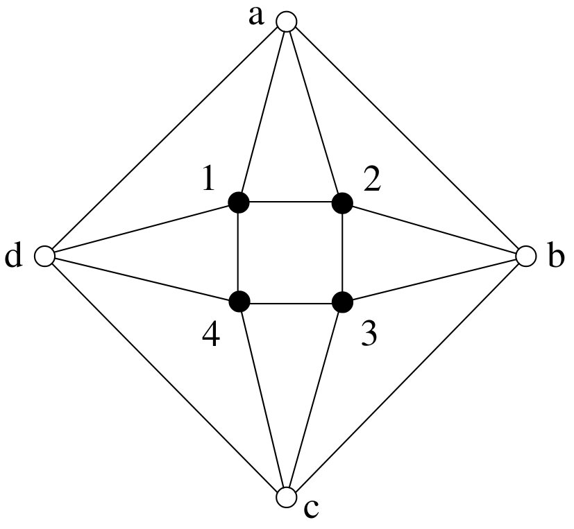 Figure 1
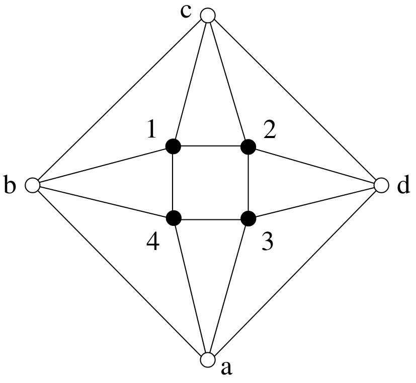 Figure 2
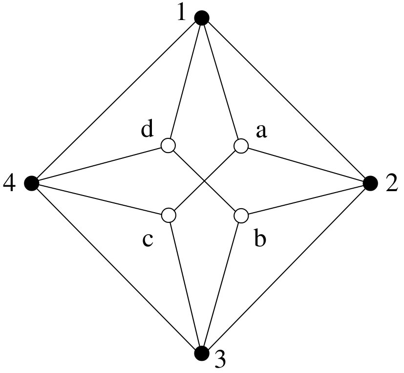 Figure 3
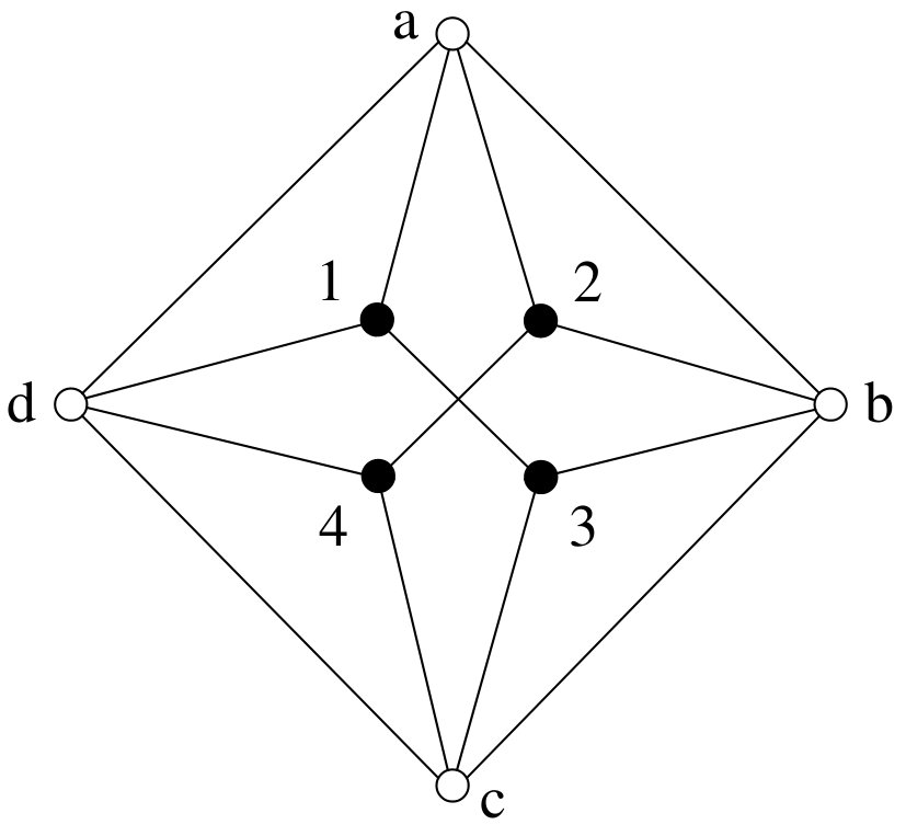 Figure 4
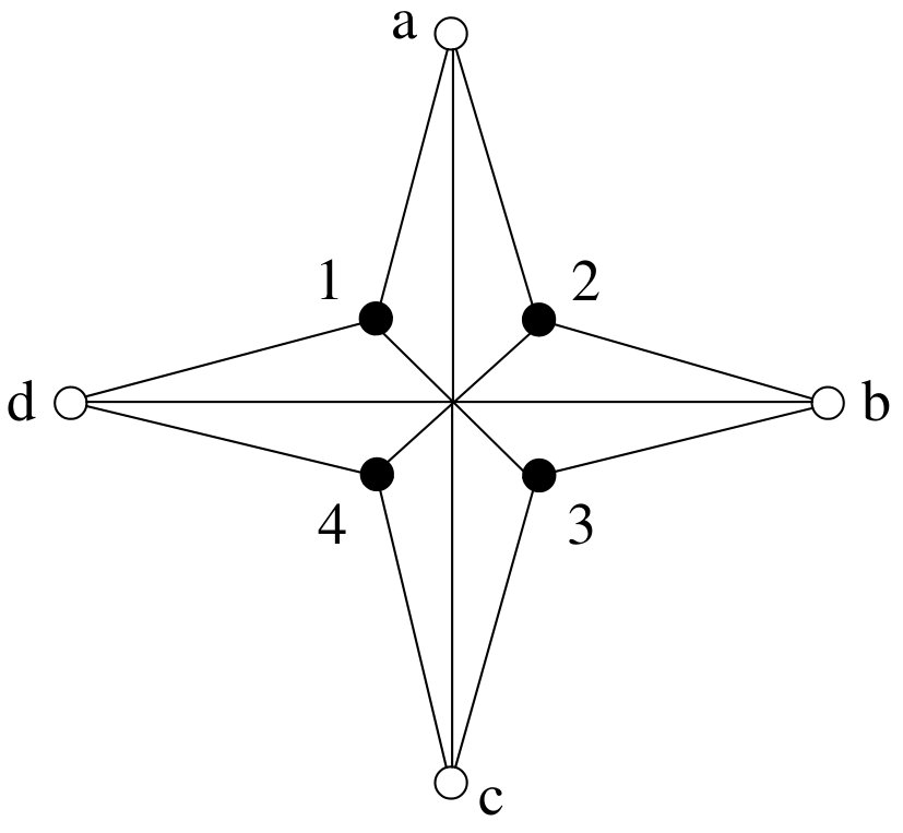 Figure 5
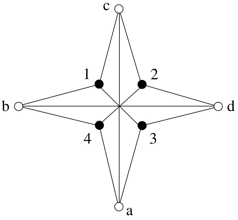 Figure 6
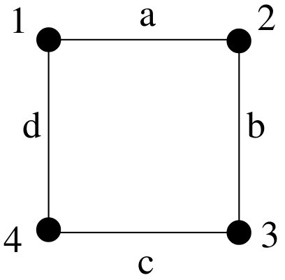 Figure 7
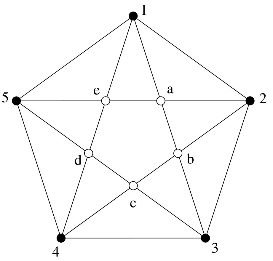 Figure 8
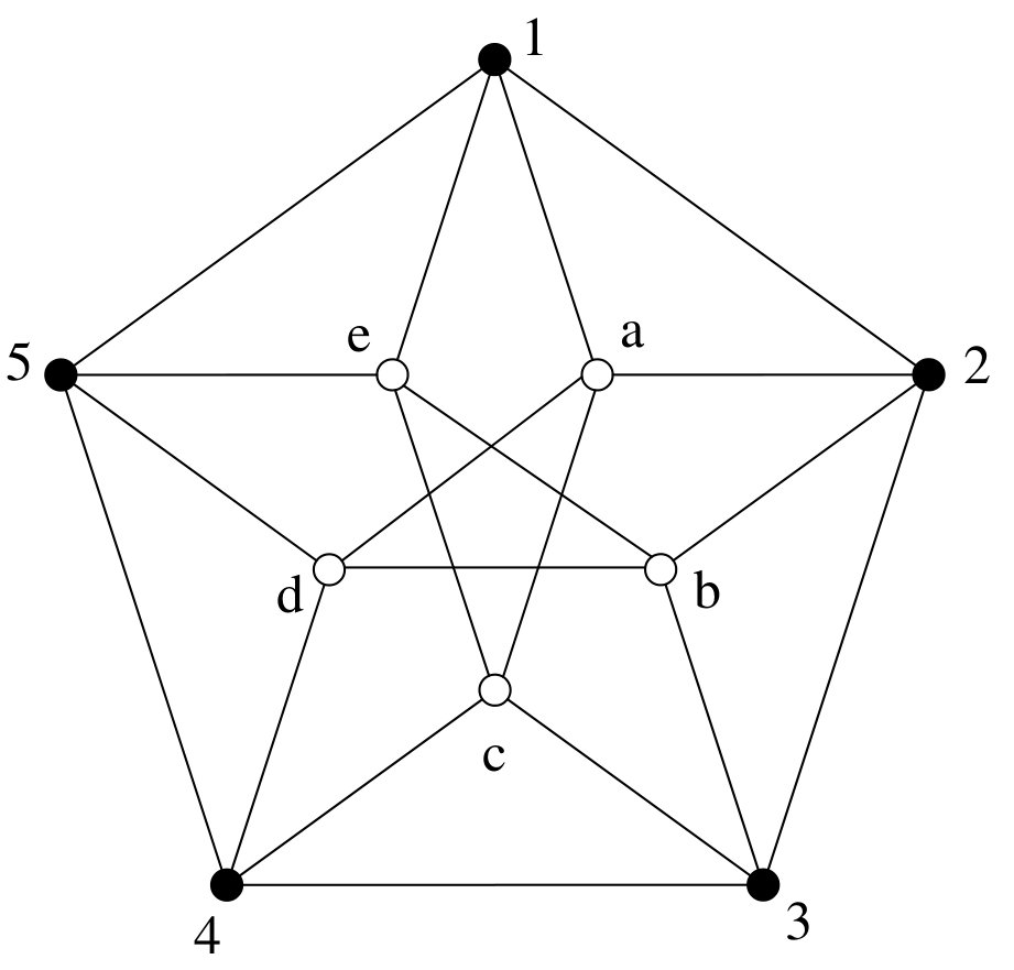 Figure 9
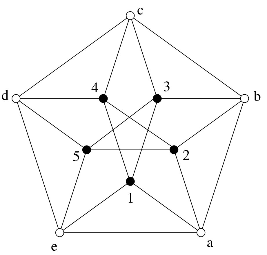 Figure 10
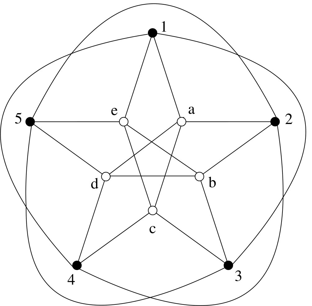 Figure 11
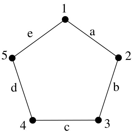 Figure 12
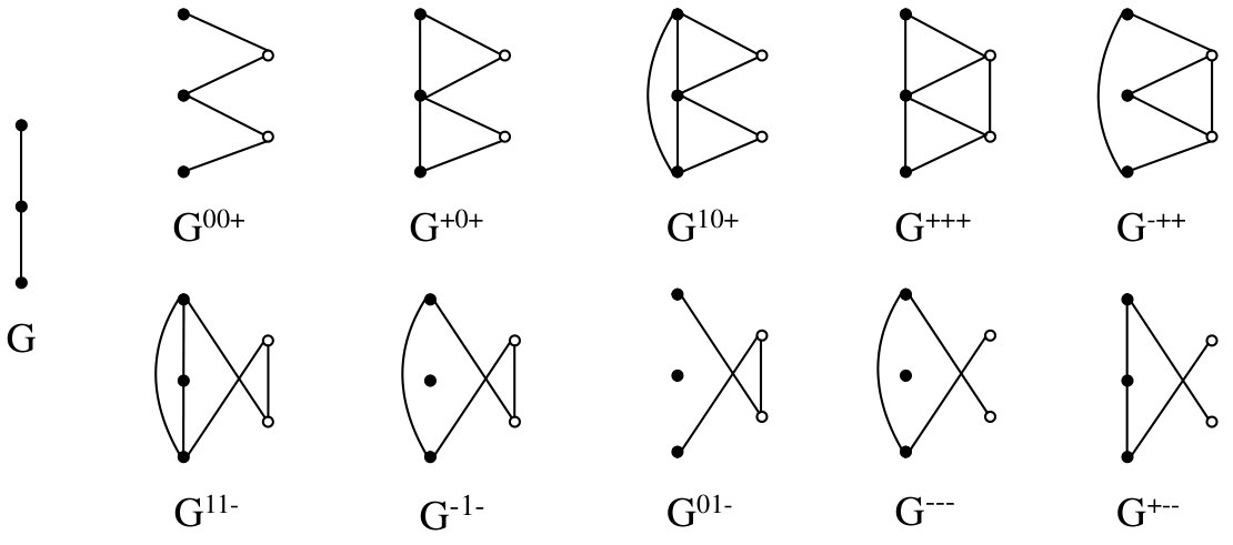 Figure 13