On the maximal halfspace depth of permutation-invariant distributions on the simplex
Davy Paindaveine, Germain Van Bever

TL;DR
This paper calculates the maximum halfspace depth for permutation-invariant distributions on the probability simplex, using stochastic ordering results originally applied to the Behrens-Fisher problem, advancing understanding of distribution depth in high-dimensional probability spaces.
Contribution
It introduces a method to compute maximal halfspace depth for a specific class of distributions on the simplex, linking stochastic ordering to distribution depth analysis.
Findings
Derived explicit formulas for maximal halfspace depth.
Connected stochastic ordering results to distribution depth computations.
Extended the application of stochastic ordering beyond traditional contexts.
Abstract
We compute the maximal halfspace depth for a class of permutation-invariant distributions on the probability simplex. The derivations are based on stochastic ordering results that so far were only showed to be relevant for the Behrens-Fisher problem.
Click any figure to enlarge with its caption.
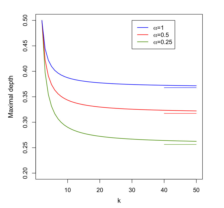 Figure 1
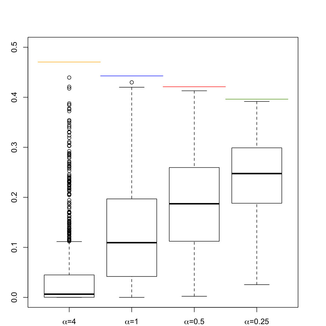 Figure 2
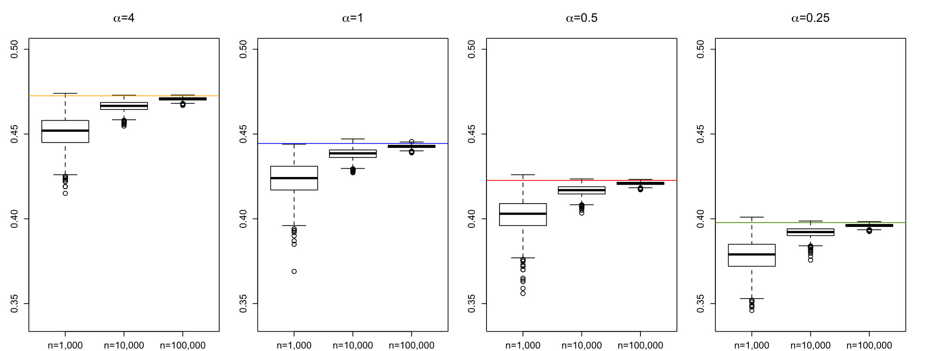 Figure 3
Peer Reviews
No public reviews on file for this paper yet. If you reviewed it on a platform where reviews are public (OpenReview, ICLR, NeurIPS, ICML), you can paste yours below so the community can read it here.
Videos
No videos yet. Explain this paper in a talk, walkthrough, or lecture? Add one.
Taxonomy
TopicsStatistical Distribution Estimation and Applications · Bayesian Methods and Mixture Models · Probability and Risk Models
On the Maximal Halfspace Depth of Permutation-invariant Distributions on the Simplex
Davy Paindaveine111Corresponding author ([email protected])
Germain Van Bever
Université libre de Bruxelles, ECARES and Département de Mathématique, CP 114/04, 50, Avenue F.D. Roosevelt, B-1050 Brussels, Belgium
Abstract
We compute the maximal halfspace depth for a class of permutation-invariant distributions on the probability simplex. The derivations are based on stochastic ordering results that so far were only showed to be relevant for the Behrens-Fisher problem.
keywords:
-unimodality , Dirichlet distribution , Halfspace depth , Majorization , Stochastic ordering
††journal: some journal
1 Introduction
Denoting as the unit sphere in , the Tukey (1975) halfspace depth H\!D(\theta,P)=\inf_{u\in\mathcal{S}^{k-1}}P\big{[}u^{\prime}(X-\theta)\geq 0\big{]} measures the centrality of the -vector with respect to a probability measure over . Any probability measure admits a deepest point, that generalizes to the multivariate setup the univariate median; see, e.g., Proposition 7 in Rousseeuw and Ruts (1999). Parallel to the univariate median, this deepest point is not unique in general. Whenever a unique representative of the collection of ’s deepest points is needed, the Tukey median , that is defined as the barycentre of , is often considered. The convexity of (see, e.g., the corollary of Proposition 1 in Rousseeuw and Ruts, 1999) implies that has maximal depth. The depth of is larger than or equal to ; see Lemma 6.3 in Donoho and Gasko (1992).
In this paper, we determine the Tukey median and the corresponding maximal depth for a class of permutation-invariant distributions on the probability simplex . The results identify the most central location for some of the most successful models used for compositional data. They have also recently proved useful in the context of depth for shape matrices; see Paindaveine and Van Bever (2017).
The outline of the paper is as follows. In Section 2, we define the class of distributions we will consider and state a stochastic ordering result on which our derivations will be based. In Section 3, we state and prove the main results of the paper. Finally, in Section 4, we illustrate the results through numerical exercises and we shortly comment on open research questions.
2 Preliminaries
Let be the collection of cumulative distribution functions such that (i) and (ii) is concave on . In other words, collects the cumulative distribution functions of random variables that are (i) almost surely positive and (ii) unimodal at [math]. Any in admits a probability density function that is non-increasing on .
For an integer and in , consider the random -vector
[TABLE]
where are mutually independent and have cumulative distribution function . The corresponding probability measure over will be denoted as . Obviously, the random vector takes its values in the probability simplex . This includes, for example, the Dirichlet distribution with parameter , obtained for the cumulative distribution function of the Gamma distribution (that corresponds to the probability density function on , where is the Euler Gamma function). The unimodality constraint in (ii) above imposes to restrict to . Note that, irrespective of , the mean vector of is .
To state the stochastic ordering result used in the sequel, we need to introduce the following notation. For -vectors with , we will say that is majorized by if and only if, after permuting the components of these vectors in such a way that and (possible ties are unimportant below), , for any ; see, e.g., Marshall et al. (2011). For random variables and , we will say that is stochastically smaller than () if and only if for any . To the best of our knowledge, the following stochastic ordering result so far was only used in the framework of the Behrens-Fisher problem; see Hájek (1962), Lawton (1968), and Eaton and Olshen (1972).
Lemma 1** (Eaton and Olshen, 1972)**
Let be a random variable with a cumulative distribution function in . Let be exchangeable positive random variables that are independent of . Then, for any such that is majorized by .
In Eaton and Olshen (1972), the result is stated in a vectorial context that requires the -unimodality concept from Olshen and Savage (1970). In the present scalar case, the minimal unimodality assumption in Eaton and Olshen (1972) is that is -unimodal about zero, which, in view of Lemma 2 in Olshen and Savage (1970), is strictly equivalent to requiring that is unimodal about zero.
3 Main results
Our main goal is to determine the Tukey median of the probability measure and the corresponding maximal depth. Permutation invariance of and affine invariance of halfspace depth allows to obtain
Theorem 1
The Tukey median of is .
Proof of Theorem 1. Let be a point maximizing and let be the corresponding maximal depth. Of course, (if , then ). Denote by , , the permutation matrices on -vectors. By affine invariance of halfspace depth and permutation invariance of , all ’s have maximal depth with respect to . Now, for any ,
[TABLE]
Since this holds for any maximizing , the result is proved.
Note that the unimodality of about zero is not used in the proof of Theorem 1, so that the result also holds at with . In contrast, the proof of the following result, that derives the halfspace depth of the Tukey median of , requires unimodality.
Theorem 2
Let have distribution with . Then, H\!D(\mu_{k},P_{k,F})=P\big{[}X_{k1}\geq 1/k\big{]}.
The proof requires the following preliminary result.
Lemma 2
For any positive integer , let h_{k,F}=P\big{[}X_{k1}\geq 1/k\big{]}, where has distribution with . Then, the sequence is monotone non-increasing.
Proof of Lemma 2. Since is majorized by the -vector , Lemma 1 readily provides
[TABLE]
which establishes the result.
Note that this result shows that, for any in , the maximal depth, , in Theorem 2 is monotone non-increasing in , hence converges as goes to infinity. Clearly, the law of large numbers and Slutzky’s theorem imply that in distribution, so that converges to as goes to infinity. In particular, for , the limiting value is , where is Gamma distributed.
We can now prove the main result of this paper.
Proof of Theorem 2. We are looking for the infimum with respect to in , or equivalently in , of
[TABLE]
where we wrote . Without loss of generality, we may assume that , which implies that . Actually, if , then all ’s must be equal to , which makes the probability equal to one. Since this cannot be the infimum, we may assume that , which implies that . Therefore, denoting as the largest integer for which , we have . Then, letting s_{m}(u)=\sum_{\ell=1}^{m}\big{(}u_{\ell}-\bar{u}\big{)}, we may then write
[TABLE]
where , and , are nonnegative and satisfy and
[TABLE]
Since is unimodal at zero and since is majorized by , Lemma 2 yields
[TABLE]
where the lower bound is obtained for and , that is, for arbitrary and . Now, since is majorized by for any , the same result provides
[TABLE]
with the lower bound obtained for , , that is, for , . Therefore, the global minimum is the minimum of , , which, in view of Lemma 2, is . This establishes the result.
Figure 1 plots the maximal depth as a function of for several , where still denotes the cumulative distribution function of the Gamma() distribution. In accordance with Lemma 2, the maximal depth is decreasing in and is seen to converge to the limiting value that was obtained below that lemma. For any , the maximal depth is equal to if and only if , which is in line with the fact that the (non-atomic) probability measure is (angularly) symmetric about if and only if ; see Rousseeuw and Struyf (2004). Interestingly, thus, the asymmetry of for would typically be missed by a test of symmetry that would reject the null when the sample (Tukey) median is too far from the sample mean.
4 Numerical illustration
We conducted two numerical exercises to illustrate Theorems 1 and 2, both in the trivariate case . In the first exercise, we generated random locations from the uniform distribution over (that is the distribution associated with the Gamma() distribution of the ’s; see, e.g., Proposition 2 in Bélisle, 2011). Our goal is to compare, for various values of , the depths , with the depth . For each , these depth values were estimated by the depths , , and , computed with respect to the empirical measure of a random sample of size from (these sample depth values were actually averaged over mutually independent such samples). For each , Figure 2 reports the boxplots of the resulting estimates of , , and marks the estimated value of . The results clearly support the claim in Theorem 1 that .
In the second numerical exercise, we generated, for various values of and , a collection of mutually independent random samples of size from the distribution . For each sample, we evaluated the halfspace depth of with respect to the corresponding empirical distribution . Figure 3 provides, for each and , the boxplot of the resulting depth values. Clearly, the results, through the consistency of sample depth, support the theoretical depth values provided in Theorem 2. Actually, while the theorem was only proved above for (due to the unimodality condition in Lemma 1), these empirical results suggest that the theorem might hold also for . The extension of the proof of Theorem 2 to further distributions is an interesting research question, that requires another approach (simulations indeed reveal that Lemma 1 does not hold if the cumulative distribution function of is with ). Of course, another challenge is to derive a closed form expression for for an arbitrary . After putting some effort into this question, it seemed to us that such a computation calls for a more general stochastic ordering result than the one in Lemma 1.
Acknowledgements
Davy Paindaveine’s research is supported by the IAP research network grant nr. P7/06 of the Belgian government (Belgian Science Policy), the Crédit de Recherche J.0113.16 of the FNRS (Fonds National pour la Recherche Scientifique), Communauté Française de Belgique, and a grant from the National Bank of Belgium. Germain Van Bever’s research is supported by the FC84444 grant of the FNRS.
The reference list from the paper itself. Each links out to its DOI / PubMed record.
- 1Bélisle (2011) Bélisle, C., 2011. On the polygon generated by n 𝑛 n random points on a circle. Statist. Probab. Lett. 81, 236–242.
- 2Donoho and Gasko (1992) Donoho, D. L., Gasko, M., 1992. Breakdown properties of location estimates based on halfspace depth and projected outlyingness. Ann. Statist. 20, 1803–1827.
- 3Eaton and Olshen (1972) Eaton, M. L., Olshen, R. A., 1972. Random quotients and the Behrens-Fisher problem. Ann. Math. Statist. 43, 1852–1860.
- 4Hájek (1962) Hájek, J., 1962. Inequalities for the generalized Student’s distribution and their applications. In: Select. Transl. Math. Statist. and Probability, Vol. 2. American Mathematical Society, Providence, R.I., pp. 63–74.
- 5Lawton (1968) Lawton, W. H., 1968. Concentration of random quotients. Ann. Math. Statist. 39, 466–480.
- 6Marshall et al. (2011) Marshall, A. W., Olkin, I., Arnold, B. C., 2011. Inequalities: theory of majorization and its applications, 2nd Edition. Springer Series in Statistics. Springer, New York.
- 7Olshen and Savage (1970) Olshen, R. A., Savage, L. J., 1970. A generalized unimodality. J. Appl. Probab. 7, 21–34.
- 8Paindaveine and Van Bever (2017) Paindaveine, D., Van Bever, G., 2017. Tyler shape depth. ar Xiv:1706.00666.