A Closed-Form Model for Image-Based Distant Lighting
Mais Alnasser, Hassan Foroosh

TL;DR
This paper introduces a closed-form mathematical model for image-based lighting that efficiently computes realistic lighting effects from environment images, enabling faster rendering with full spectrum color adaptation.
Contribution
It derives a novel closed-form solution for the light integral equation applicable to various BRDFs, improving speed and accuracy over traditional methods.
Findings
Achieves an order of magnitude faster rendering times.
Provides noise-free, spectrum-aware lighting calculations.
Supports multiple BRDF models like Lambertian and Phong.
Abstract
In this paper, we present a new mathematical foundation for image-based lighting. Using a simple manipulation of the local coordinate system, we derive a closed-form solution to the light integral equation under distant environment illumination. We derive our solution for different BRDF's such as lambertian and Phong-like. The method is free of noise, and provides the possibility of using the full spectrum of frequencies captured by images taken from the environment. This allows for the color of the rendered object to be toned according to the color of the light in the environment. Experimental results also show that one can gain an order of magnitude or higher in rendering time compared to Monte Carlo quadrature methods and spherical harmonics.
Click any figure to enlarge with its caption.
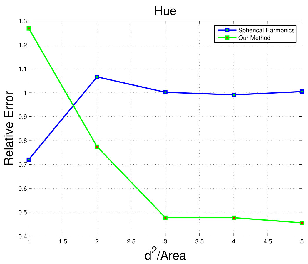 Figure 1
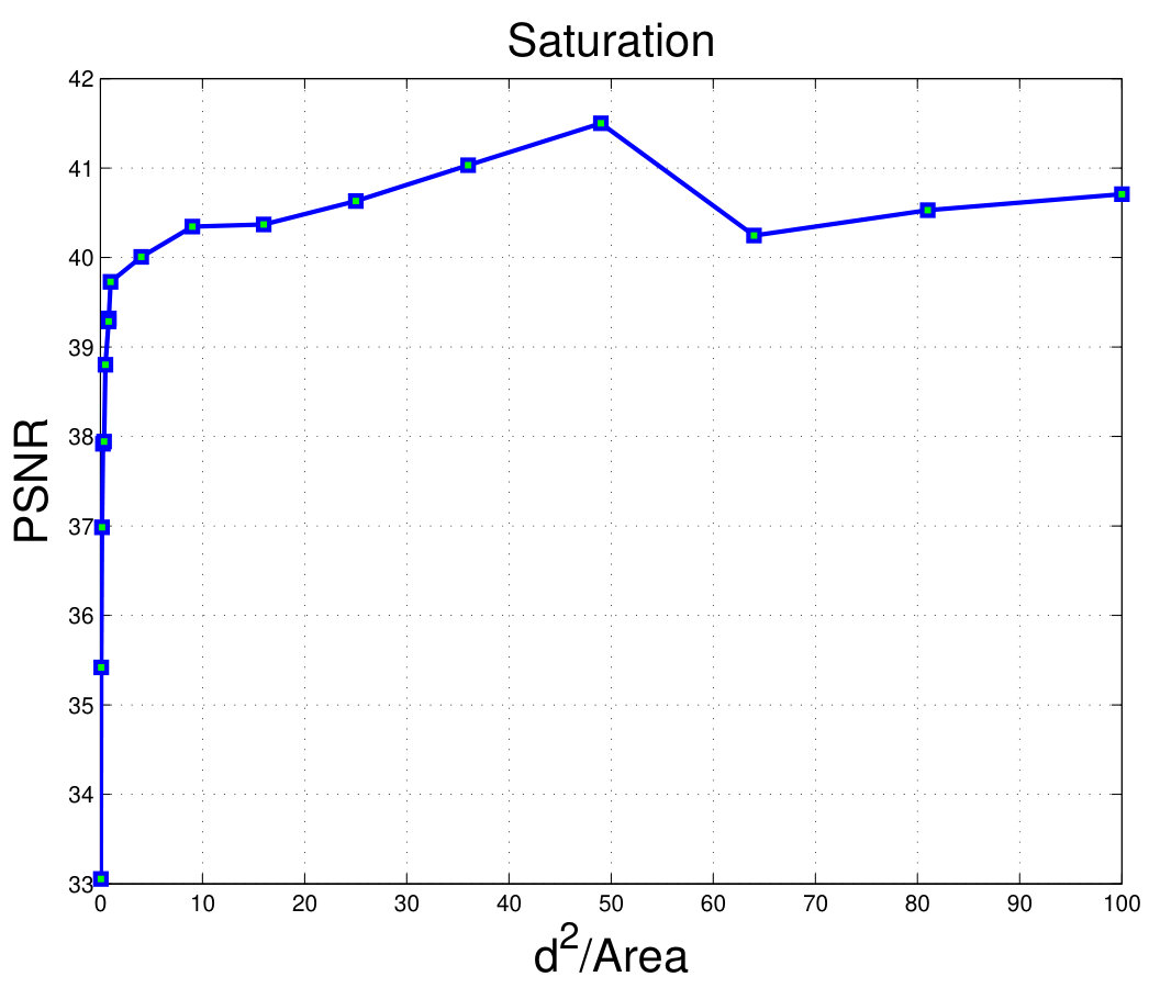 Figure 2
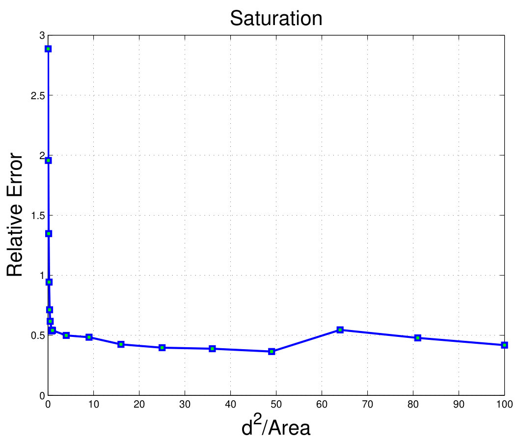 Figure 3
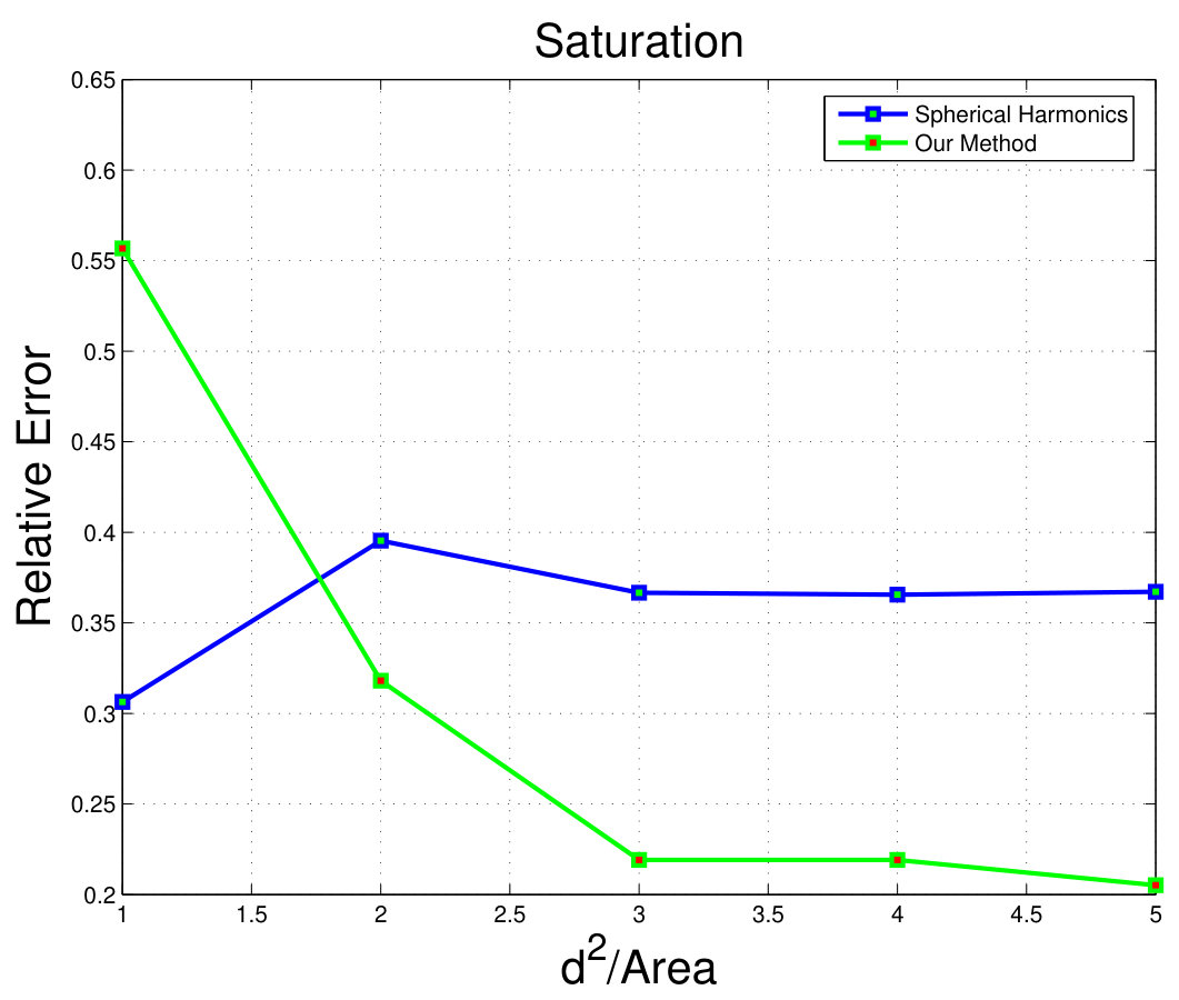 Figure 4
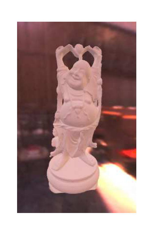 Figure 5
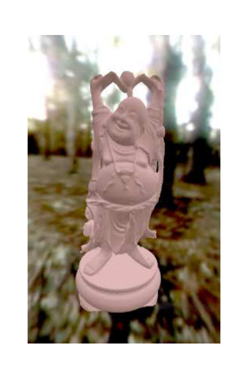 Figure 6
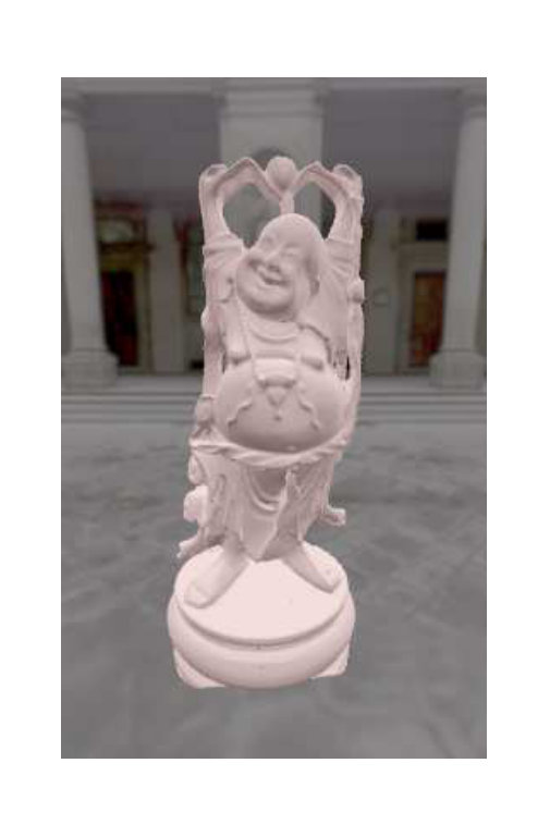 Figure 7
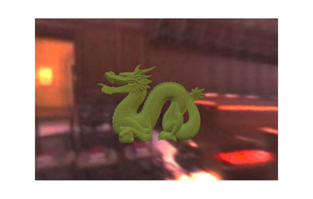 Figure 8
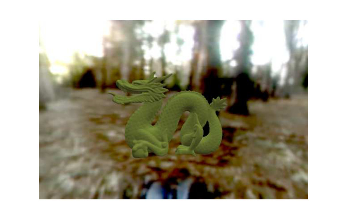 Figure 9
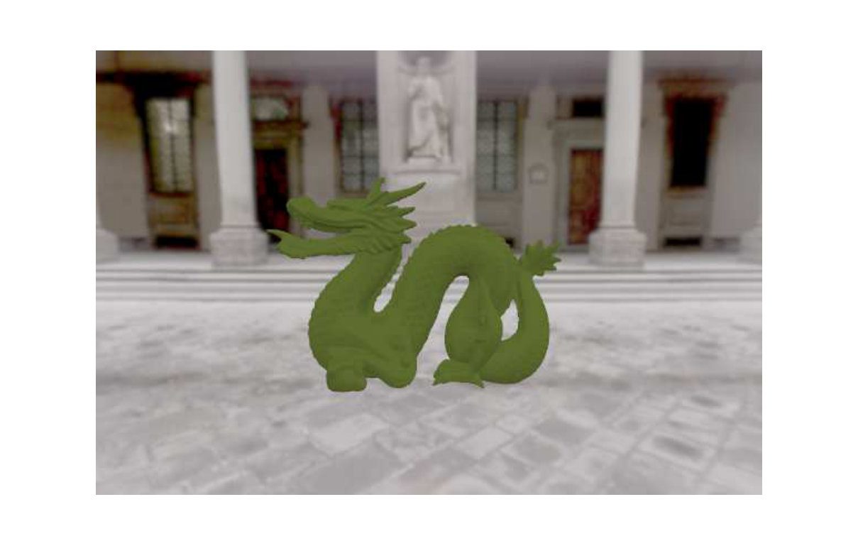 Figure 10
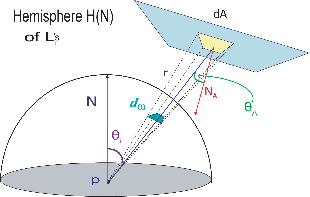 Figure 11
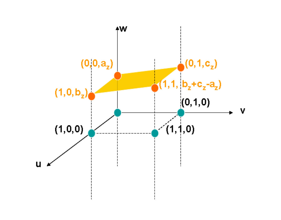 Figure 12
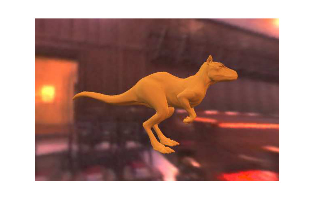 Figure 13
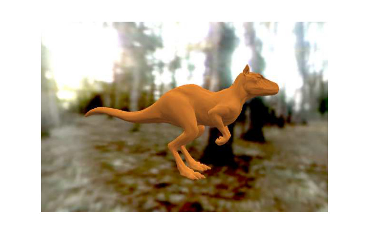 Figure 14
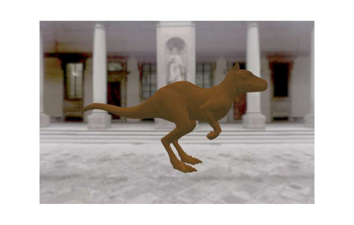 Figure 15
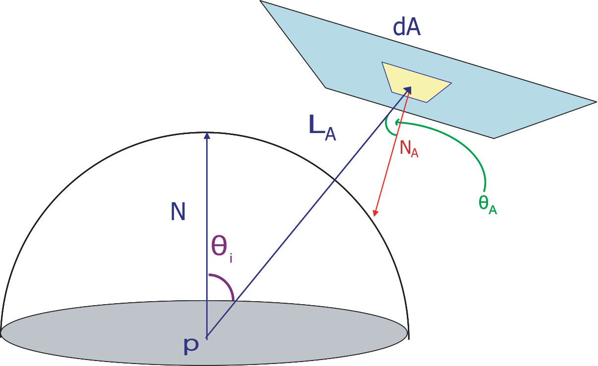 Figure 16
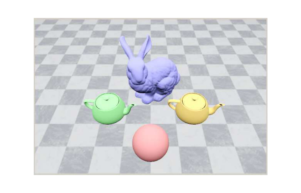 Figure 17
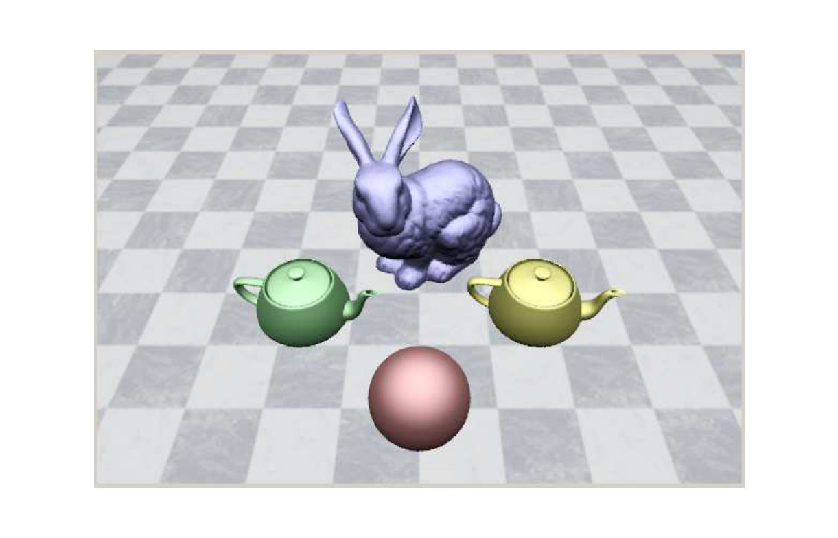 Figure 18
 Figure 19
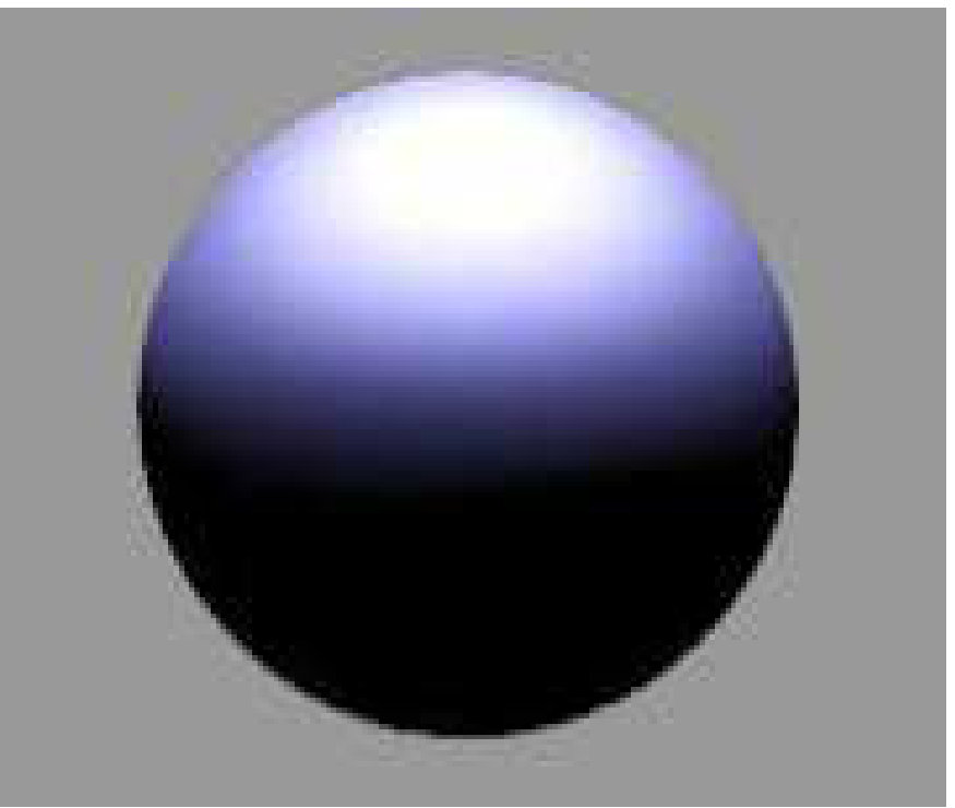 Figure 20
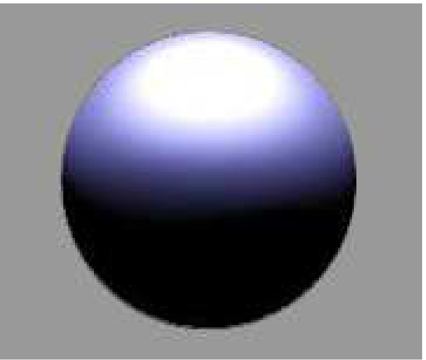 Figure 21
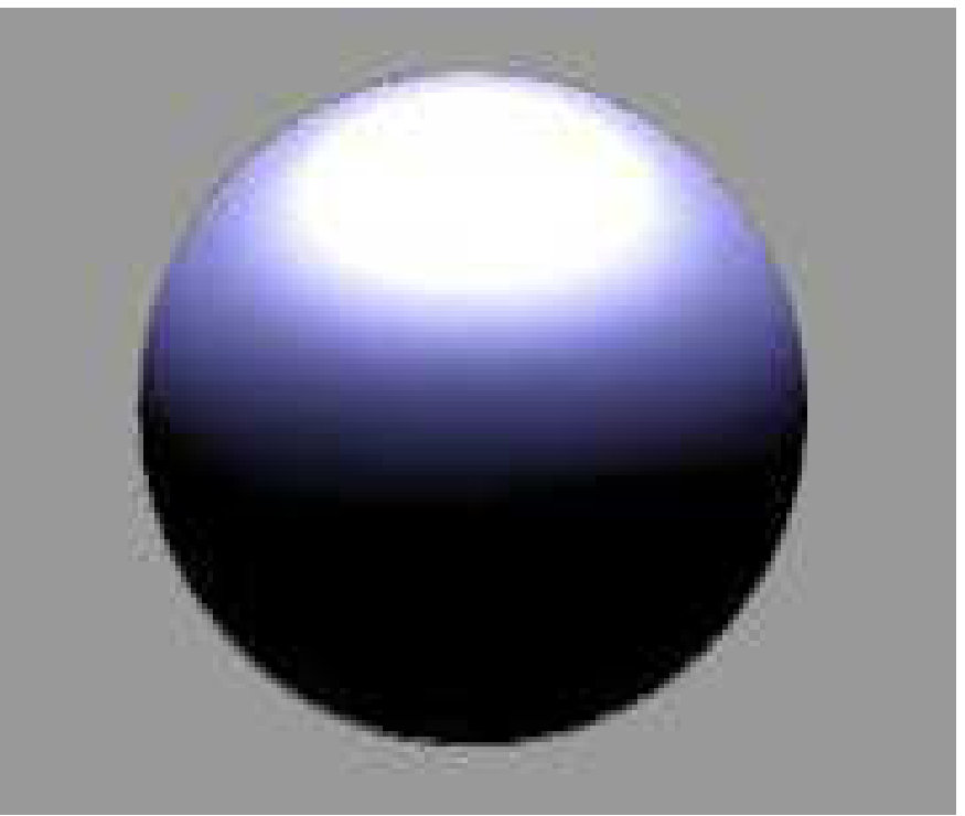 Figure 22
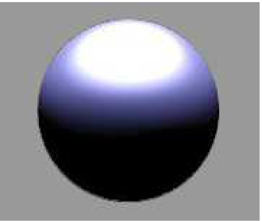 Figure 23
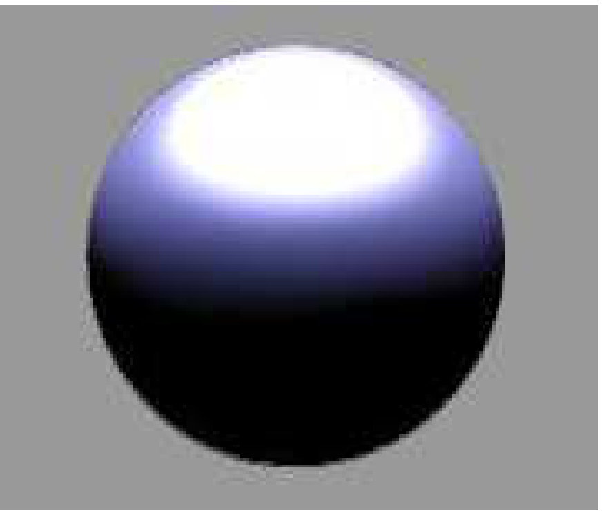 Figure 24
 Figure 25
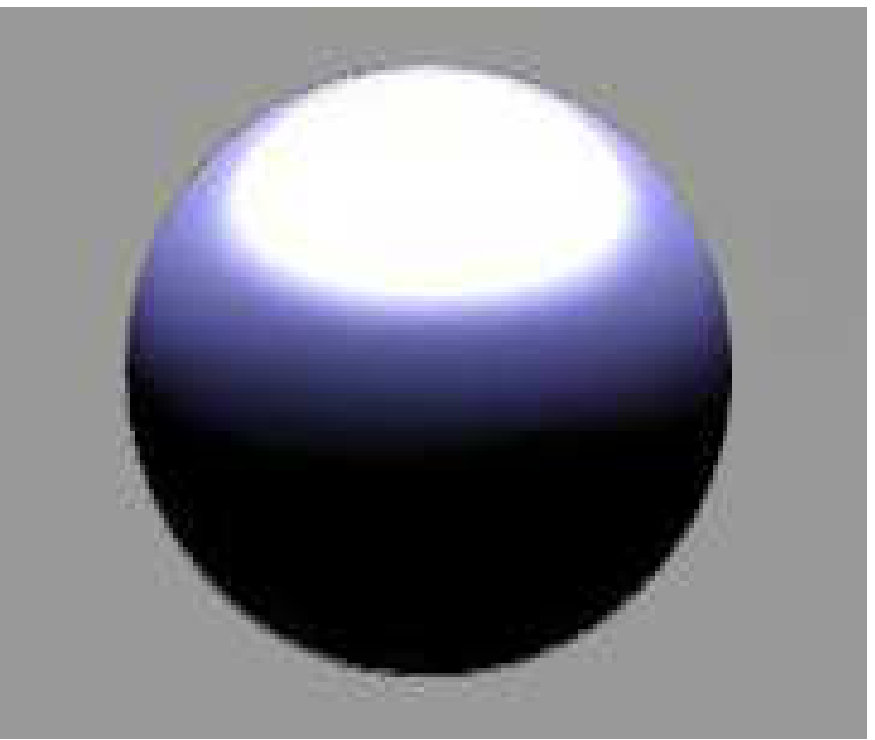 Figure 26
| , , | ||||||||
| , | 0 | 0 | ||||||
| , , | ||||||||
| , | 0 | 0 | 1 | |||||
| , , | ||||||||
| , | 0 | 0 | 0 | 1 | 1 | |||
| , , | ||||||||
| , | 0 | 1 | 0 | |||||
| , , | ||||||||
| , | 0 | 1 | 0 | 1 | 1 | |||
| , , | ||||||||
| , | 0 | 1 | 0 | 0 | 1 | |||
| , , | ||||||||
| , | 1 | 0 | 0 | 1 | 1 | |||
| , , | ||||||||
| , | 1 | 0 | 1 | |||||
| , , | ||||||||
| , | 1 | 0 | ||||||
| , , | ||||||||
| , | 0 | 1 | 1 | |||||
| , , | ||||||||
| , | 0 | 1 | ||||||
| , , | ||||||||
| , | 1 | 1 |
| RGB: Relative Error | HSI: Relative Error | HSI: SNR (dB) |
|---|---|---|
| R=0.0075% | H=0.0161% | H=42.5401 |
| G=0.0075% | S=0.3614% | S=54.9891 |
| B=0.0049% | I=0% | I= |
Peer Reviews
No public reviews on file for this paper yet. If you reviewed it on a platform where reviews are public (OpenReview, ICLR, NeurIPS, ICML), you can paste yours below so the community can read it here.
Videos
No videos yet. Explain this paper in a talk, walkthrough, or lecture? Add one.
Taxonomy
TopicsComputer Graphics and Visualization Techniques · Advanced Vision and Imaging · Remote Sensing in Agriculture
A Closed-Form Model for Image-Based
Distant Lighting
Mais Alnasser and Hassan Foroosh Mais Alnasser was with the Department of Computer Science, University of Central Florida, Orlando, FL, 32816 USA at the time this project was conducted. (e-mail: [email protected]).Hassan Foroosh is with the Department of Computer Science, University of Central Florida, Orlando, FL, 32816 USA (e-mail: [email protected]).
Abstract
In this paper, we present a new mathematical foundation for image-based lighting. Using a simple manipulation of the local coordinate system, we derive a closed-form solution to the light integral equation under distant environment illumination. We derive our solution for different BRDF’s such as lambertian and Phong-like. The method is free of noise, and provides the possibility of using the full spectrum of frequencies captured by images taken from the environment. This allows for the color of the rendered object to be toned according to the color of the light in the environment. Experimental results also show that one can gain an order of magnitude or higher in rendering time compared to Monte Carlo quadrature methods and spherical harmonics.
Index Terms:
Image-Based Relighting, Distant Light Modeling, Light Integral Equation, Lambertian and Phong models
I Introduction
Image-based rendering (IBR) has been an active area of research in computational imaging and computational photography in the past two decades. It has led to many interesting non-traditional problems in image processing and computer vision, which in turn have benefited from traditional methods such as shape and scene description [38, 37, 146, 95, 101, 2, 1, 56, 3, 36, 54, 83, 34, 69, 11, 72, 78, 135, 85, 134, 15, 137, 76, 75, 77, 71, 70, 16, 10, 132], scene content modeling [80, 79, 86, 87, 84, 88, 142, 141, 143, 140, 139], super-resolution (in particular in 3D) [67, 110, 118, 113, 46, 32, 114, 94, 108, 104, 105, 109, 106, 31, 120, 33, 68, 111, 112, 117], video content modeling [126, 17, 12, 136, 122, 133, 18, 121, 124, 13, 14, 35, 123, 125, 9], image alignment [65, 60, 29, 30, 6, 19, 20, 116, 61, 115, 26, 25, 64, 24, 62, 58, 107, 23, 21, 59, 57], tracking and object pose estimation [129, 97, 99, 119, 98], and camera motion quantification and calibration [45, 43, 51, 81, 40, 42, 39, 73, 82, 50, 63, 74, 90, 91, 92, 8, 89, 96, 27, 41, 41, 49], to name a few.
Using images to estimate or model environment light for relighting objects introduced or rendered in a scene is a central problem in this area [47, 48, 127, 28, 144, 100, 4, 5, 66, 22, 145, 44]. This requires solving the light integral equation (also known as the rendering equation), which plays a crucial role in IBR. One of the oldest and most straightforward approaches for solving the integral is to approximate the solution using the Monte Carlo method [93]. However, Monte Carlo is an estimation method, and unless sufficient light samples are taken, it produces noisy results. Therefore, a substantial number of samples and accordingly more time is typically required in order to render a realistic low-noise image.
The key idea that we propose in this paper is the fact that any light source can be modeled as an area light source. For instance, a spot light or a directional linear light can both be modeled as special cases of an area light source, where the dimensionality has reduced. Similarly, environment lighting using cubemaps may be viewed as the limiting case of pointwise varying multiple area light sources. Therefore, in this paper, we first show how the light integral can be solved in closed-form for a constant area light source of rectangular shape. We apply our solution to rendering lambertian and Phong-like materials. We then extend our solution to non-constant pointwise varying light sources and apply our solution to lambertian surfaces. In order to streamline the understanding of the implementation issues, we also provide a pseudocode for our algorithm.
Because of the closed-form nature of our solution, no sampling is required and noise is completely eliminated. On the other hand, the lack of requirement for sampling reduces the rendering time significantly, making it dependent only on the complexity of the object (i.e. the number of triangles used to represent it) for a constant area light source, and dependent on the required highest light frequency in the case of pointwise varying environment lighting. In particular, in the case of low-frequency environment lighting, we achieve the same level of accuracy as spherical harmonics with coefficients reduced by an order of magnitude in O(1) complexity. A very simple preprocessing of the light is required, to compress it using discrete cosine transform, which also happens to be the most classical tool for image compression.
II Related Work
Some very interesting closed-form solutions have already been proposed to solve the light integral. The appeal of closed-form solutions lies in the fact that they provide complete elimination of noise. Furthermore, the availability of a closed-form solution expedites the rendering process significantly. For estimation methods such as Monte Carlo [128], many samples of the environment are required to render realistic low-noise images. On the other hand, several hours might be required to generate one single image.
Currently, the closed-form solutions proposed in the literature mostly target specific scenarios. For example, the work done in [102] targets linear light sources and provides a solution to the integral for diffuse and specular materials lit by such a light. The work done by Arvo [7] provides analytic solutions to the light integral for polyhedral sources using the irradiance jacobian. [130] introduced the use of B-splines to represent surface radiance in static scenes. A recent work by Sun et al [131] provides a closed-form solution to the light integral given isotropic point light sources. Their solution targets the scenarios of fog, mist and haze.
Closed-form solutions were also proposed for special cases of non-constant lighting such as the work done by [52], which provides a solution for linearly-varying luminaires. The most common application for non-constant lighting is in environment maps. [103] used spherical harmonics to solve the light integral for diffuse materials lit by environment maps, and achieved real-time rendering.
The methods used to solve the light integral vary and so do the scenarios for which the light integral is solved. In addition to advantages described in the previous section in terms of compression and speed, one of our contributions is to provide a unified framework that works for spot light, area, and natural distant environment lighting. We achieve this by formulating a new closed-form solution to the lighting integral. Our framework works for lambertian and Phong-like materials. Mirrored, transmissive and textured materials can be easily embedded within the framework. We were able to achieve a constant complexity for lambertian materials depending only on the resolution of the rendered image, suggesting real-time if implemented on hardware.
III Solving the Light Integral
Figure 1 shows the relationship between the incident light and the light leaving the surface of an object at a given point. The following is the the most general form of the light integral describing this relationship:
[TABLE]
where is the outgoing direction, is the emitted light at point in the direction , is the radiance leaving the surface at a point in the direction , is the Bidirectional Reflectance Distribution Function (BRDF), is the incident radiance emitted from the area patch , is the angle between the unit normal at the point and the vector from to the patch , is the angle between the unit normal of the patch and the light direction, is the distance between the point and the patch , is the hemisphere of directions around the normal .
In the following sections, we describe our approach to provide closed-form solutions to this integral equation. We first develop our approach for lambertian and Phong-like materials in the case of a rectangular constant area light source, which can naturally reduce to a point or a linear spot light sources. We then show that the same approach extends readily to multiple area light sources with pointwise varying color and intensity, leading thus to a unified framework that also applies to distant environment lighting using cubemaps.
III-A Constant Area Light Sources
We start with this case, because its solution shows the underlying concepts in our approach, from which either specific or more general cases are derived. We derive this case for lambertian and Phong-like materials in the following sections.
III-A1 Lambertian Materials
The case for perfectly diffusing Lambertian materials is shown in Figure 2. For lambertian materials, the integral assumes its simplest form:
[TABLE]
which can also be written as
[TABLE]
where is the material albedo as a function of the point , is the light intensity, is the unit normal to the surface at point , is the unit normal to the patch , is the opposite direction of the light emitted by the patch , is the angle between and , is the angle between and , is the distance between the point and the patch .
Let be the squared average distance between the area light source and the point . For typical distant light sources, can be replaced in practice by with negligible error, in which case the integral reduces to
[TABLE]
To simplify the above integral, we transform the endpoints , and of the area light source and its unit normal such that the surface point is at the origin and the surface unit normal at the point is along the Z-axis. We denote the transformed endpoints by , and , and the transformed normal by .
Let be the center of the patch after applying the transformation, then is the vector . Since is transformed to the point , becomes the vector , which reduces the integral to
[TABLE]
Since and , we have , and the integral becomes
[TABLE]
The point on the rectangular area light source can be described in parametric form by , where . The integral now becomes
[TABLE]
The above formula contains a max term that needs to be eliminated in order to be able to integrate in closed-form. The key observation that allows us to do this is the fact that is the equation of a plane as shown in Figure 3. As and vary in the unit interval, a plane segment is defined, whose corners are given by
[TABLE]
The max term can be eliminated by identifying the portion of this plane segment that lies above the plane , i.e. by setting the bounds and of the integral such that only the portion above the plane is taken into account. This is verified per point on the object being rendered. There are two trivial cases. The first is when all of the plane segment is above the plane . In this case, the bounds would be , and . The second case would be it is all under the plane . In this case the integral evaluates to zero.
Table I shows the bounds for each of the other cases, where , and . Note that the bounds of the integral are given in terms of the transformed coordinates of the end points of the area light source, which are known values. For some cases, the integral has to be divided into two subintegrals. For those cases the bounds for the first subintegral are denoted by , , and and the bounds for the second subintegral are denoted by , , and .
Once the bounds of the integral are determined as discussed above, the max term is simply eliminated by the fact that we would be integrating only for the cases where is always strictly positive. Rearranging the terms in the integral then would yield
[TABLE]
[TABLE]
which is simply an integral of a polynomial that can be easily evaluated in closed-form. The resultant solution can then be embedded in the rendering code achieving a complexity of O(1).
III-A2 Phong-Like Materials
For Phong-like materials the light integral becomes as follows:
[TABLE]
Where is the albedo, is the shininess of the material, and is the reflection of the viewing vector at a point on the surface.
Substituting with , the integral becomes
[TABLE]
For Phong-like materials, we similarly transform the endpoints , and of the area light source and its unit normal such that the surface point is at the origin and the reflection vector at the point is along the z-axis.
To simplify the integral, we proceed as we did with the Lambertian materials. The integral becomes
[TABLE]
Again, to eliminate the max term, we divide the integral into the same cases mentioned above. The integral now becomes
[TABLE]
Using the trinomial expansion
[TABLE]
The integral then reduces to
[TABLE]
Rearranging the terms, the integral finally becomes
[TABLE]
[TABLE]
which is a sum of integrals of polynomials that can be again readily evaluated in closed-form achieving a complexity of O() for Phong-like materials.
III-B Non-Constant Area Light Sources
In the previous sections, we derived closed-form solutions for rendering various types of materials lit by a constant area light source of rectangular shape. These solutions reduce to a point spot light or a linear spot light source by simple dimensionality reduction. Therefore, our close-form solutions nicely include other popular light source models. To demonstrate that our approach is general, we now show that it can also be equally extended to provide a solution for direct lighting in scenes lit by environment cubemaps. Indeed, from the point of view presented in this paper, each side of a cubemap is simply an area light source with pointwise varying color and intensity. Therefore, we would simply require to extend the results in the previous sections to the case of non-constant area light sources.
We demonstrate the basic idea for Lambertian materials, which can also be extended in a similar manner as before to other types of material. For Lambertian materials the light integral becomes
[TABLE]
Following the same steps as before the integral can be simplified to
[TABLE]
[TABLE]
where is the varying light color and intensity, which is essentially a pixel in an image of a cubemap.
This integral can be solved in closed-form only if we can provide a closed-form expression for the pixel value . A natural way to do this would be to use some basis function. In principle, any basis may be used to compute . However, we used the Discrete Cosine Transform (DCT), since it provides two advantages. First, combined with the light integral equation, it lends itself to a closed-form solution, second DCT is a well established and widely used compression tool. Therefore is given by an inverse cosine transform of a set of coefficients precomputed by preprocessing the image in the cubemap, as follows:
[TABLE]
[TABLE]
The ’s are the DCT coefficients. The coefficients are precomputed for each color channel and are stored as a cubemap that is used as an input to our rendering equation in (III-B). The preprocessing step requires time, if we use coefficients.
Upon substituting from (III-B) into (III-B), our integral becomes
[TABLE]
We then rearrange the integral to get the following
[TABLE]
A closed-form solution can now be found for the integral part of the above equation, which we denote by . The closed form generated will have divisions by the constants , , and . However, at i=0 and j=0 these constants evaluate to zero, leading to divisions by zero. To solve this problem, the integral is divided into four cases:
Case 1: and
[TABLE] 2. 2.
Case 2: and
[TABLE] 3. 3.
Case 3: and
[TABLE] 4. 4.
Case 4: and
[TABLE]
which is the same as the constant area light source for lambertian materials case.
The above integrals can now be evaluated using the bounds in table-2 and the color value at a point on a Lambertian surface will be
[TABLE]
where,
[TABLE]
The number of coefficients generated by the discrete cosine transform of the image is equal to the image resolution . If desired, all coefficients can be used to compute in O(MN) time, or alternatively we can truncate the coefficients to some desired cut-off low frequency values trading between accuracy and speed.
The nature of our closed-form solution allows our algorithm to work for high frequency as well as low frequency. Another significant advantage is that we are able to achieve realistic shading using only one coefficient per face, reducing the number of coefficients needed to achieve realistic shading as compared to spherical harmonics.
If O(1) complexity is desired, the analytic solution for the lambertian surfaces under constant lighting can be used, such that .
IV Results and Discussion
We have applied and verified our method under various lighting scenarios for lambertian and Phong-like materials. For constant lighting Figure 6 displays Lambertian and Phong-like materials under such lighting. Figure 10 demonstrates the variations in the shininess of the material lit by an area light source. Figures 10, 10 and 10 show examples of rendering lambertian objects in different environments. As mentioned earlier, all lambertian objects are rendered at O(1) time complexity. For environment lighting, one can readily see in Figures 10, 10 and 10 that our method realistically captures the effect of colors in the environment on the rendered objects.
To evaluate the quality of our results, we performed three sets of experiments. The first set establishes the error associated with the approximation that led to our closed-form solution, i.e. the assumption that the distance between the point being shaded and the light patch is constant and equal to the average distance. We varied the ratio of the squared distance over the area of the light source, , and generated ground truth images under illumination with area light sources at finite distances, using the Monte Carlo technique with more than 1000 samples. Then, images under the exact same lighting conditions were generated using our method. The images were compared with the ground truth in the HSI domain to avoid the color channel correlations of the RGB model. Figures 4 - (a) and (b) show the results for the Saturation channel. As for the Hue and Intensity channels, we found 0% error indicating that for our method they are independent of the ratio . As shown in these figures, the peak-signal-to-noise ratio (PSNR) increases as a function of , or equivalently the relative error reduces as this ratio increases. Note that the PSNR increases sharply to about 40dB for , and remains approximately stable thereafter. Note also that even for small values of , the PSNR for our method has a remarkably high value of over 33dB.
In the second set of experiments, we generated ground truth images by rendering a lambertian sphere in several cubemaps, i.e. under distant environment lighting. We then rendered images of the sphere under the same lighting using our method. We tested for both SNR and relative error against the ground-truth generated by Monte Carlo, and averaged over a large number of environments. Results are summarized in Table II. We observed that for lambertian materials the lower-bound in the relative error (or the upper-bound for SNR) is achieved with one coefficient per face in our method. In other words, we achieve our best result with the DC value of the cosine transform, and our method is almost invariant to the frequency of light in the case of lambertian material.
In the third set of experiments, we generated ground truth images for multiple environments using Monte Carlo, with more than 1000 samples. We generated images under the same environments using Spherical Harmonics and our method. The error was computed against the ground truth provided by Monte Carlo. Figures 5- (a) and (b) show the results for one of the environments used in the experiment. By examining the figures one can tell that our method provides more accurate results than Spherical Harmonics.
In summary, we first formulated a novel approach to provide closed-form solutions to the light integral for lambertian and Phong-like materials, which are lit by constant area light sources. Spot light and directional linear light sources are then special cases of our formulation. Using the key observation that a cubemap can be represented as six non-constant area light sources, we have also shown that the same framework can be extended to provide a closed-form solution to environment lighting. In our formulation, the cut-off frequency of the light can be chosen arbitrarily at any desired value in the cosine transform domain. In particular, for lambertian material, we only require one DCT coefficient per face to render realistic images, achieving a complexity of O(1). Also, we gain an order of magnitude or higher in rendering time compared to classical environment sampling techniques such as Monte Carlo.
In principle, models of other material types can be formulated within our framework and solved in similar fashions. Another direction of research could be the incorporation of general BRDFs. One issue that needs to be considered is the rendering of shadows. In classical estimation techniques based on sampling, shadowing is implicitly incorporated. In our framework, due to the closed-form nature of our solution, shadows need to be computed explicitly. However, several methods have already been proposed in the existing literature [53, 55, 138] for efficient and realistic computation of shadows that would nicely fit in our framework.
Appendix
The following is pseudo code for implementing the algorithm. It is intended to provide a global understanding of our algorithm.
For each point to be rendered
if (lambertian){
Transform the end points of the light source , and and its normal such that the point is at the origin and the unit normal at the point is along the z-axis.
Compute , , , , ,
if( and and and )
if(Constant)
item
call formula for constant_diff_case1.
else
item
for each of the six faces of the cube map call formula for nonconstant_diff_case1.
else if( and and and )
if(Constant)
item
call formula for constant_diff_case2.
else
item
for each of the six faces of the cube map call formula for nonconstant_diff_case2.
else if(…)
:
else if(( and and and )
return 0
}
else if(specular){
Transform the end points of the light source , and and its normal such that the point is at the origin and the reflection vector at the point is along the z-axis.
Compute , , , , ,
if( and and and )
call formula for constant_spec_case1.
if( and and and )
call formula for constant_spec_case2.
else if(…)
:
else if( and and and )
return 0
}
The reference list from the paper itself. Each links out to its DOI / PubMed record.
- 1[1] Muhamad Ali and Hassan Foroosh. Natural scene character recognition without dependency on specific features. In Proc. International Conference on Computer Vision Theory and Applications , 2015.
- 2[2] Muhamad Ali and Hassan Foroosh. A holistic method to recognize characters in natural scenes. In Proc. International Conference on Computer Vision Theory and Applications , 2016.
- 3[3] Muhammad Ali and Hassan Foroosh. Character recognition in natural scene images using rank-1 tensor decomposition. In Proc. of International Conference on Image Processing (ICIP) , pages 2891–2895, 2016.
- 4[4] Mais Alnasser and Hassan Foroosh. Image-based rendering of synthetic diffuse objects in natural scenes. In Proc. IAPR Int. Conference on Pattern Recognition , volume 4, pages 787–790, 2006.
- 5[5] Mais Alnasser and Hassan Foroosh. Rendering synthetic objects in natural scenes. In Proc. of IEEE International Conference on Image Processing (ICIP) , pages 493–496, 2006.
- 6[6] Mais Alnasser and Hassan Foroosh. Phase shifting for non-separable 2d haar wavelets. IEEE Transactions on Image Processing , 16:1061–1068, 2008.
- 7[7] James Arvo. The irradiance Jacobian for partially occluded polyhedral sources. In Computer Graphics Proceedings, Annual Conference Series, ACM SIGGRAPH, pages 343–350, July 1994.
- 8[8] Nazim Ashraf and Hassan Foroosh. Robust auto-calibration of a ptz camera with non-overlapping fov. In Proc. International Conference on Pattern Recognition (ICPR) , 2008.