Discretization of SU(2) and the Orthogonal Group Using Icosahedral Symmetries and the Golden Numbers
Robert V. Moody, Jun Morita

TL;DR
This paper explores discretizing the SU(2) group using icosahedral symmetries and golden ratios, resulting in a structured approach for approximating elements of SU(2) with potential applications in quantum computing.
Contribution
It introduces a novel discretization of SU(2) based on icosahedral symmetries and golden numbers, providing an efficient method for approximating SU(2) elements.
Findings
The constructed root system has a natural structure of SU(2, R).
The reflection group H^∞ is of index 2 in O(4, R).
Any SU(2) element can be approximated using five fixed reflections.
Abstract
The vertices of the four dimensional -cell form a non-crystallographic root system whose corresponding symmetry group is the Coxeter group . There are two special coordinate representations of this root system in which they and their corresponding Coxeter groups involve only rational numbers and the golden ratio . The two are related by the conjugation . This paper investigates what happens when the two root systems are combined and the group generated by both versions of is allowed to operate on them. The result is a new, but infinite, `root system' which itself turns out to have a natural structure of the unitary group over the ring (called here golden numbers). Acting upon it is the naturally associated infinite reflection group , which we prove is…
Click any figure to enlarge with its caption.
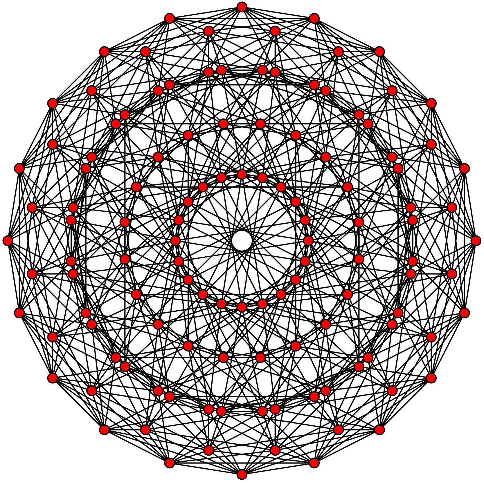 Figure 1
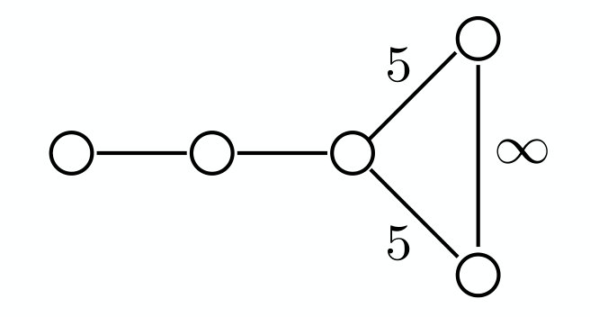 Figure 2
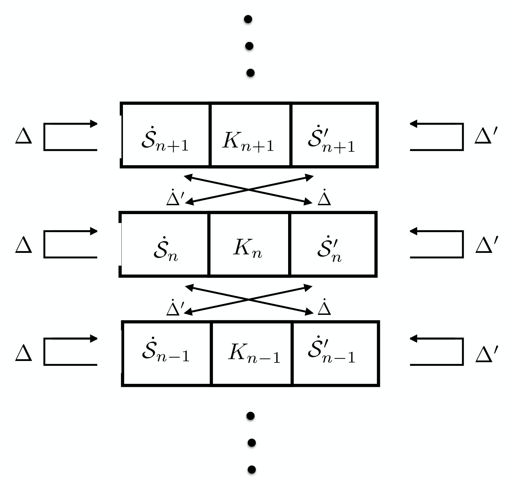 Figure 3
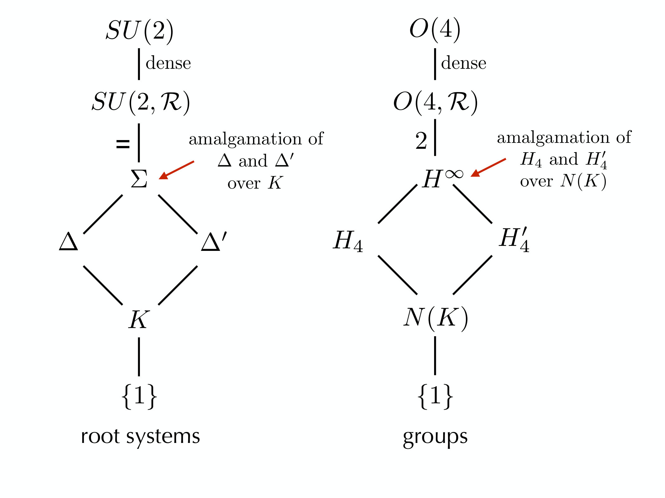 Figure 4
Peer Reviews
No public reviews on file for this paper yet. If you reviewed it on a platform where reviews are public (OpenReview, ICLR, NeurIPS, ICML), you can paste yours below so the community can read it here.
Videos
No videos yet. Explain this paper in a talk, walkthrough, or lecture? Add one.
Discretization of SU(2) and the orthogonal group using icosahedral symmetries and the golden numbers
Robert V. Moody & Jun Morita
(March 15, 2024)
Abstract
The vertices of the four-dimensional -cell form a non-crystallographic root system whose corresponding symmetry group is the Coxeter group . There are two special coordinate representations of this root system in which they and their corresponding Coxeter groups involve only rational numbers and the golden ratio . The two are related by the conjugation . This paper investigates what happens when the two root systems are combined and the group generated by both versions of is allowed to operate on them. The result is a new, but infinite, ‘root system’ which itself turns out to have a natural structure of the unitary group over the ring (called here golden numbers). Acting upon it is the naturally associated infinite reflection group , which we prove is of index in the orthogonal group . The paper makes extensive use of the quaternions over and leads to a highly structured discretized filtration of . We use this to offer a simple and effective way to approximate any element of to any degree of accuracy required using the repeated actions of just five fixed reflections, a process that may find application in computational methods in quantum mechanics.
Department of Mathematics and Statistics, University of Victoria, Victoria, BC., V8W 3R4 Canada Department of Mathematics, University of Tsukuba, Tsukuba, Ibaraki, 305-8571, Japan.
E-mail: [email protected], [email protected]
Keywords: icosahedral symmetry, non-crystallographic root systems, infinite reflection groups, discretization of , golden numbers, quaternions
1 Introduction
The symmetry group of the icosahedron (and the dodecahedron) is the icosahedral group, denoted here, with elements. It is a finite Coxeter group, that is to say, it is a finite group generated by reflections and Coxeter relations, and it is simply transitive on the simplicial cells into which the icosahedron is partitioned by the mirrors of the reflections in . Apart from numerous dihedral groups, there are only two finite indecomposable non-crystallographic Coxeter groups: and its big sister , which is the symmetry group of the four-dimensional regular polytope called the -cell (and its dual, the -cell). This paper involves both these groups, but notably the latter.
The -cell has vertices and three-dimensional faces, see Fig. 1. The vertices form a root system, of type . With this interpretation of the vertices as roots, the set of reflections in these roots (opposite roots give the same reflection) is the entire set of reflections in the group , and they generate it. The order of the group is . Notice that we use the symbol both as an adjective signifying the type of root system involved and as a noun signifying the reflection group generated by the roots of that system. We will do the same thing with .
Both and involve the golden ratio and its algebraic conjugate in all sorts of significant ways. For instance, there is the well-known model of the vertices of the -cell [5] §20 and §27, or equivalently the roots of the root system of type , as the set of points
[TABLE]
Here the first component of the label refers to the power of appearing in the denominators of the components and the second component is used to distinguish the rational versus irrational nature of (some of) the components.
One cannot help noticing the interesting fact that only even permutations are allowed in the third type of root. Half of the potential permutations are missing. The other half can be obtained by conjugating these roots by interchanging and throughout. Of course doing so produces another model of the root system of type , and the reflections in these generate a second model of the Coxeter group . We shall also use the notation and , that suggests the origin of these groups as reflection groups.
It is tempting to look at the group generated by the reflections of , but one quickly realizes that this group, let’s call it (or ) is infinite.111Throughout the paper we will see parallel structures pertaining to the three-dimensional setting around and the four-dimensional setting around . Generally we use the same symbol for the corresponding objects, but if the context does not make it clear then we shall make the distinction as in , , , , , , etc. Since all the points of the set
[TABLE]
lie on the sphere of radius in , which is compact, is certainly not a discrete set. Up to now no one seems to have paid much attention to it.
The objective of this paper is to get some idea of what and look like. In fact they have some very attractive features, as we shall see. Not surprisingly is a dense set of points on the unit -sphere in , see Prop. 3.7. It is also a group under quaternion multiplication, and we shall show that it is an amalgamation of and , each of which is itself a group. Similarly is an amalgamation of the two groups and . What is especially interesting is that using and allows us to explicitly approximate elements of the two groups and , the unitary and special orthogonal groups of and respectively, by elements with matrix coefficients of the form (we call them dyadic integers from the field ). In fact the matrices used all arise from the reflections of which are the ones involving and , and even from just reflections if one gets down to the level of root system bases. The approximation can be made as fine as one wishes (with increasing powers of two in the denominators) and there is a simple and efficient algorithm for doing it.
The key to all of this is to interpret as the standard division ring of quaternions, and use the fact that its unit sphere can be identified with and that it can be made to act as on the three-dimensional subspace of pure imaginary quaternions (those which change their sign under quaternionic conjugation).
The paper is primarily concerned with the picture, but we also require information from the corresponding, and essentially parallel situation based on the three-dimensional icosahedral root system and its corresponding conjugate system . The arguments are not identical but sufficiently parallel that we provide only sketches of the arguments for the three-dimensional case.
The paper is organized around understanding the structure of the root system and the group that the reflections in its roots generate. The approximation results appear in the final section, though they can be read directly after §3.
Icosahedral symmetry and the Coxeter groups have continued to intrigue people from ancient times until the present day, where they are now familiar in such diverse places as carbon molecules, buckyballs, the capsids (outer shells) of viruses, Penrose tilings, and the aperiodic order of quasicrystals. There remains continuing interest in the mathematical world too, for instance, [6] which investigates the subgroup structure of in a quaternionic context, and [3] which explores some of the ways of making affine extensions of the root systems, following the success of affinization of the root systems of the simple Lie algebras. Affinization is accomplished by extending the Coxeter diagram, and might be thought of as based on using translations to extend root systems. In the present paper, although the root systems involved are defined intrinsically from the and root systems and the Galois conjugation , effectively the result is to extend by using contractions. Indeed this contractive aspect is something seems worthy of fuller study.
We might note here that there have been considerable advances in the understanding of Coxeter groups along with their associated geometrical meanings by using the Clifford algebras, see [4] and its associated references. Although we have not used these ideas here, and indeed we require only a very limited number of tools, the Clifford algebra approach may offer new insights into the setting we are introducing.
2
The set of roots of the root system of type can be presented in the standard form of (1) as the union of three types of vectors in . We let denote the set of roots of types R[0,0] and R[1,0], which form a crystallographic root system of type , and for the set of roots of type R[1,1]. Of course these distinctions are not intrinsic to the root system itself, but only to our coordinatization of it. However this distinction plays a fundamental role in what is to follow.
Along with we have its conjugate which is the set of conjugates of , and the corresponding sets and (it being irrelevant whether or not the dot operators are applied before or after conjugation). .
The reflections in the roots generate the group we call . It is a Coxeter group of type . Similarly we have generated by the reflections in the roots of , also of type . We are primarily interested in the group which is generated by and together. The reflections given by , the roots in common to both systems, generate a subgroup of type For example
[TABLE]
is a base (with either choice of the sign).
We let denote the unit sphere in -space. Both and are in , and so too is the set . It is the smallest subset containing and closed under its own reflections (i.e. if and is the reflection in then ).
We note the important fact that
[TABLE]
At the start we use only the algebraic consequences of reflections applied in the context of and , but later we will interpret everything in the real quaternions, where the elements that we are discussing can be interpreted as elements of SU.
It is useful to keep in mind the basic facts about :
[TABLE]
The quotient ring is the Galois field of elements. Let denote the natural homomorphism of . The elements of are . We extend the meaning of the map to its component-wise version .
Inside the -vector space , define to be the subspace spanned by the elements of taken modulo , i.e., . This is a -dimensional space with basis and . We define and . Note the cardinalities: , , and .
Similarly we have using and the corresponding subset . As we have already mentioned, and this sentence suggests, and will be true throughout, everything we say will come in two versions, which are interchanged by conjugation. Henceforth we will usually only state and give proofs for one of the versions, understanding that the other will be equally true.
With the obvious dot product on we find that is totally isotropic. This is just another way of saying that for all , . In addition, if and are linearly dependent, then . This simply follows from .
We have parallel statements for and . However, for any and we always have .
Proposition 2.1**.**
- (i)
. In particular, for all , ;
- (ii)
for all and , . In particular if and then .
∎
3 as a reflection group
The set of vectors
[TABLE]
define reflections that correspond to the Coxeter diagram of Fig. 2 and these reflections generate . Indeed they contain a set of generators for both of the Coxeter groups and . The associated Gram matrix with entries is positive semidefinite with null vector . Certainly is a factor of the corresponding Coxeter group, and later on we shall see that it is a proper factor, see Prop. 8.1.
Proposition 3.1**.**
If satisfies
[TABLE]
then one of the three following cases prevails:
[TABLE]
In the language and notation introduced above, these three cases correspond to
[TABLE]
Proof: Modulo each . Their squares are modulo . A quick check shows that the sum of four such elements can be zero modulo if and only if one of the three conditions of the thesis is true. ∎
Examples of all three types occur when we double each of the roots, i.e. when we look at .
Corollary 3.2**.**
The three-dimensional version of Prop. 3.1 reads: if satisfies
[TABLE]
then one of the two following cases prevails:
[TABLE]
∎
For define the spherical sets
[TABLE]
and
[TABLE]
and similarly the conjugated versions using . We call here the level of the spherical set. We define
[TABLE]
so , and similarly .
To these we add
[TABLE]
the set of roots of type R[0,0].
Here are two consequences of Prop. 3.1:
Proposition 3.3**.**
, and .
Proof: Let . Then and satisfies . Using Prop. 3.1, one can hunt through all solutions to see that only elements of can satisfy this, and then restrict to filter them out to . ∎
Proposition 3.4**.**
For ,
[TABLE]
Furthermore, is in if and only if .
Proof: Let , and let be minimal so that . If then . If then and by Prop. 3.1, , see (8), from which . The reverse inclusion comes from the definitions, and the last line is clear. ∎
Proposition 3.5**.**
For all , .
Proof: Let , so by definition and . We have . The elements and are in and respectively, so in all cases . Since is not in , but only in , . However and furthermore . Thus , which is what we wished to prove. ∎
Corollary 3.6**.**
For all and for all , has infinite order.
Proof: Let . Then , , and so on. ∎
Let denote the commutator subgroup of .
Proposition 3.7**.**
- (i)
* is dense in ;*
- (ii)
* is dense in ;*
- (iii)
* is dense in .*
Proof: With and , is a rotation in the plane orthogonal to the two roots and , and by Cor. 3.6 it has infinite order. Let be the infinite cyclic group generated by . The orbit of under generated is infinite and hence is dense on the circle on the sphere . In particular has rotations through angles as small as we please.
Now also , so is a rotation of infinite order in a different plane orthogonal to and we get a second group with arbitrarily small rotations. These two groups generate a subgroup of that is a dense subgroup of the group of of rotations of . Since can certainly map to , we see that it also contains a subgroup that is a dense subgroup of the of rotations of this space. Since and generate the entire rotation group , we see that contains a dense subgroup of this space.
Now (i),(ii),(iii) are all clear. ∎
Proposition 3.8**.**
Let . Then
- (i)
for all , ;
- (ii)
* for all , and for each there exists for which ;*
- (iii)
for each there are three reflections of the form where , for which .
Proof: (i). We start with the slightly weaker assumption that . Let and .
[TABLE]
Let . Since and are elements of , . Let . As long as , , so . If then , so . By Prop. 3.4, is either in or for some .
Now whatever the case is, if then we have shown that is either in or in some or for . Now assume that . Then if it is not possible that , for either in which case by the same reasoning, is on some sphere of level at most , contrary to , or in which case has level . In the case that , then noting Prop. 3.5 we see that actually . But in fact cannot be in , since these elements do not change level under the application of and so would be impossible. Thus This proves part (i).
This last case, where the level drops under reflection, is particularly interesting and we wish to look more carefully how it can happen in (iii) below.
(ii). Let . In the notation of part (i) above, if then Now if then , and then also and the resulting . However, if then and remains in . We need to show that we can choose for which the corresponding .
For definiteness (the other cases work the same way) we assume that and write , where . We begin with , though ultimately we will cycle its last three components around. Then the question is what does it mean for
[TABLE]
to hold, or quivalently, what does it mean for ?
The latter is equivalent to , or finally
[TABLE]
This may happen, but if we cycle the last three terms of around then we get the same equation but with the coefficients likewise cycled around. Adding all three of the equations together and using the fact that we get the contradiction . Thus, for at least one of these three possibilities for , equation (11) fails, and this version of produces .
(iii). Suppose that and let . What is required to have ? To see what happens here, it is easiest to fix one particular form that can take, and we choose . All other forms are even permutations of this, and as will be seen, there is no loss in generality in assuming this form. Now for any , is some even permutation of . Referring to (10), the question becomes, how can ? Looking at the [math] in the first coordinate of , it is clear that must be one of the elements, , , or . Since an overall sign change in makes no difference to the reflection defined by nor to the equation we are trying to solve, we can replace the in each of these by simply . Doing this we find there is exactly one solution in each of the three sets.
For instance, taking the second type we have
[TABLE]
as go through the various possibilities of sign, so , gives the value we are looking for. In fact the other two solutions are just obtained by cyclically permuting the last three coordinates, so the solutions in this case are
[TABLE]
The three solutions, and only these three, produce the desired effect that , and as a consequence, as we saw above, . This concludes the proof of part (iii). ∎
It is worthwhile noting that the three vectors we have found in (13) are all in the plane orthogonal to the roots and and they lie at angles of to each other.
Let
[TABLE]
This is a ring which we shall call the ring of dyadic golden numbers.
Proposition 3.9**.**
[TABLE]
Proof: By definition (2), ). Let for all . We have . Now proceed by induction and assume that we have shown that . Then from Prop. 3.5 and Prop. 3.8(iii), . By Prop. 3.8(ii) we see that all of . Thus
[TABLE]
However Prop. 3.5 and Prop. 3.8 show that the left-hand side here is closed under the action of the reflections in the roots , and these reflections generate all of . This gives the reverse inclusion. For the final equality see Prop. 3.4.∎
Proposition 3.10**.**
For all , .
Proof: consists of the roots of , and similarly for . Now proceed by induction. We simply have to note that for each element of there are reflections arising from that will map it into images in , see Prop. 3.5. However, according to Prop. 3.8(c) each of these elements will be produced exactly three times as we use all the reflections available from . Thus , and likewise for . This completes the induction step. ∎
The consequence of Prop. 3.8 and Prop. 3.5 is that to go deeper into the structure of we need to apply reflections alternately from and . It is this path that leads to finer and finer discretization of the unitary group.
The situation that we have just described is pictorially represented in Fig. 3.
4
The four-dimensional theory that we have outlined so far has a parallel version in three dimensions around the Coxeter group . Most of the features that we have described in the four-dimensional case appear again here, but now notationally distinguished with the additional suffix ‘’. When we are dealing with both settings together, we shall also use the suffix ‘’ for the four-dimensional situation in order to avoid confusion.
The unit sphere in consists of points, namely the vectors and all permutations of its coordinates, and the points and all permutations of these coordinates. If in the second set of points we restrict them by allowing only even (= cyclic) permutations then they provide points which together with the original , produce a set of points which may be viewed as the non-crystallographic root system of type . They are the vertices of the icosadodecahedron. The reflection group generated by the distinct reflections in these points, now called roots, that is the reflections in the mirrors (planes) through the origin orthogonal to these roots, is the icosahedral group of order .
As a base for the root system of type we can use the vectors , , .
Instead of the even permutations of we can conjugate them, thus taking only all the even permutations of (or equivalently we take all the odd permutations) and do the same thing. We then end up with , the set of conjugates of the elements of . Again we have a root system of type and again the reflections in these roots generates a copy of the icosahedral group.
We write for the non-rational roots of , and similarly for .
Let denote the group generated by the reflections in and let be the orbit of under . We shall see that is a dense set of points on the unit -sphere .
We put this into the -dimensional setting in which we have discussed by considering the -dimensional space here as the subspace . Then it is clear that and , and indeed all of , lies in . In fact we shall see that .
Later on we shall put everything into the setting of the algebra of quaternions , at which point will be come the subspace of pure quaternions.
As before, let and let denote the natural homomorphism of . In place of we will now wish to use . It is often convenient to identify this with the subspace of , and we will do this when it is useful to do so.
Using this we define the analogues of and , namely
[TABLE]
which will play the same role as and in the four-dimensional case. Written as elements of
[TABLE]
and similarly for . Define , and similarly .
The dot product on is defined by for all , which matches the dot product it has as a subspace of . From Prop. 2.1 we have:
Proposition 4.1**.**
- (i)
. In particular, for all , ;
- (ii)
for all and , . In particular if and then .
∎
We now obtain very similar results to those of §3. We mainly just list these, the proofs being basically the same. However, there is one significant difference that appears immediately—there are no longer two spherical sets to deal with. For , we define
[TABLE]
and similarly using . We call here the level of the spherical set. The sets and have no relevant counterparts if since
[TABLE]
To these we add
[TABLE]
It is clear that and , and parallel statements for .
As a consequence of Cor. 3.2:
Proposition 4.2**.**
- (i)
;
- (ii)
for all ,
[TABLE]
Furthermore, is in if and only if . ∎
For each , we also have and the reflection in taken in is just the restriction of the reflection taken in restricted to . We use the same symbol for both, with context distinguishing them if necessary. Corresponding primed notation will be used for . denote the groups generated by the reflections of and respectively. We may think of these groups as subgroups of and .
From Prop. 3.5 we have
Proposition 4.3**.**
For all , . ∎
Corollary 4.4**.**
For all and for all , has infinite order. ∎
Following the arguments of Prop. 3.7 we have
Proposition 4.5**.**
- (i)
* is dense in ;*
- (ii)
* is dense in ;*
- (iii)
* is dense in .*
∎
Define . It is now rather easy to use the four-dimensional results of §3 to deduce corresponding results about the three-dimensional situation. We state these without further comment.
Proposition 4.6**.**
[TABLE]
Proposition 4.7**.**
For all , .
Proof: consists of the roots of , and similarly for . Now proceed by induction. We simply have to note that for each element of there are reflections arising from that will map it into images in , see Prop. 3.5. However, according to Prop. 3.8(iii) (which is actually set up so as to make the corresponding three dimensional case rather apparent) each of these elements will be produced exactly three times as we use all the reflections available from . Thus , and likewise for . This completes the induction step. ∎
5 How acts on
Proposition 5.1**.**
- (i)
* acts transitively on ;*
- (ii)
* acts transitively on ;*
- (iii)
*For each the set of roots *(elements of ) orthogonal to is a translate of by an element of ;
- (iv)
For each the stabilizer of in contains a subgroup conjugate to .
Proof: (i) It suffices to show that contains the basic roots of (6). This happens because in the Coxeter diagram of Fig. 2, is connected to the four others by chains of bonds that are all odd (namely labelled with or ). The argument is easily explained by doing it for the case of a bond labelled between two roots . Then . But the left side is also , showing that . If the sign is wrong we can use one more reflection . The proof of (ii) is similar.
(iii) The stabilizing reflections of , where , consists of all elements of , see Prop. 4.6. Parts (iii) and (iv) follow directly from this. ∎
Instead of thinking of and simply as subsets of , we can view them as subsets of the quaternion algebra . We will identify the subspace of that we have been using with the subspace of pure quaternions: . Then and similarly for . Generally we use this interpretation henceforth.
We equip with the usual conjugation which changes the signs of the last three components of each vector.222Usually the conjugation is designated by the , but that would cause confusion with our earlier notation. The usual dot product of is the standard one for , and can be expressed in terms of the quaternionic multiplication by
[TABLE]
As is well known, the unit sphere of , that is the set of vectors satisfying , can be identified with . Explicitly can be interpreted as the group by the usual matrix representation of using
[TABLE]
Returning to the ring (14), we define to be the set of all unitary matrices with coefficients in . Using (16), identifies with the set of all quaternions with coefficients in with norm , i.e. with .
is a subgroup of , and it is by Prop. 3.9. This tells us that has the natural structure of a group, namely . Furthermore, since is dense in , is dense in .
We recall that for any and any we have
[TABLE]
In particular this shows that reflection can be effected by multiplication. Since is by definition the smallest set containing and closed under its own reflections, it follows that is generated as a group by .
Now we are viewing as ordinary three-dimensional space, and since , so if and only if . Then for all and all ,
[TABLE]
showing that . This is the familiar way in which elements of turn into elements of , so that maps to the conjugation on . This is a rotation, and in this way we obtain the well-known double cover mapping
[TABLE]
However, there is more. If then for all , then , since if and then . Thus the group of rotations on the sphere in -space induced by actually acts as a group of symmetries of . In particular they all lie in .
Proposition 5.2**.**
- (i)
* is a group under quaternion multiplication and is generated by ;*
- (ii)
* and is dense in ;*
- (iii)
* acts naturally as a group of isometries on via the mapping for all ;*
- (iv)
Under the mapping in (iii), maps onto a subgroup of index in .
∎
Proof: There remains only to prove (iv). Let . We begin by making the observation that
[TABLE]
Since the mapping is and its kernel is , it is clear that the last of these rotations, , while is is in , is not something that can arise from . We shall see that this is the only obstruction that we have to deal with.
Since , maps into itself. Let denote the image of in under the mapping . Note that if and then and (17) reads
[TABLE]
Now suppose that . We wish to make as simple as possible by multiplying on the left by elements in . Consider . Since is transitive on , there exists with . Writing , (20) shows that . This being the case we can assume at the outset that . However we see from (5) that we can alter this sign, so we can actually assume that . Now, the only elements of that have the form are and , and since is an orthogonal transformation fixing and , it can only permute these two pairs roots around. Of the four possible rotations that are possible here, two of them require interchanging the two coordinate positions and changing one sign, and that requires . Thus, by composing with elements of we can reduce to one of the pair ; and indeed, . This proves that . ∎
We note that is not dense in , since the only -points on the unit circle are and . Likewise (the subgroup of all the elements of whose coefficients are in ) is not dense in —and for basically the very same reason: on is surjective onto the unit circle.
Proposition 5.3**.**
The stabilizer of in is where is the permutation operator on the last two coordinates.
Here is in its obvious form of working on the last three coordinates, that is on the space in the quaternions, and is the group generated by and .
Proof: The first observation is that in the rotation of the last three coordinates exists (as a rotation of order ) and also the changes of signs of the individual coordinates exist (as the reflections in these coordinates). The same goes for , of course. Now let be in the stabilizer of . Let and let . Then since is an isometry. Since is transitive on , there is a with . Now the element fixes both and . We can ask what does to . It must map the remaining two elements and into roots of the form . However the general form of roots shows that the only possibilities are and . The signs can be adjusted as we please by using an element from the Weyl group of , but may still interchange the two points, in other words may be the involution . We shall show in Prop. 9.1 that does not contain . ∎
6 and as groups
The two basic root systems we began with are and . The rational parts of these sets is their intersection .
Proposition 6.1**.**
, , and are groups (under quaternion multiplication) of orders respectively.
This is a well-known fact, see for instance [5] §20. But for the convenience of the reader we prove it here.
Proof: For the rational root system it is clear that the product of any two elements of is a unit vector in the rational space , and so is still in . Inversion is just quaternion conjugation, and it preserves . Thus is a group with order .
We shall prove that is a group; the proof for then follows immediately. The roots of are given in (1). The first set of these consists, in quaternion notation, of the elements . Multiplication of a quaternion on the left by turns it into . There are sign changes, but the important thing to observe is that it performs an even permutation of the coordinates, interchanging the first two coordinates and the last two coordinates. Likewise multiplication by or performs an even permutation of the coordinates (and makes two sign changes). Similar things happen if the multiplication by is on the right. In particular, left and right multiplications by map into itself.
Now apart from the elements in , every other has the property that and in . In fact is either or an even permutation of . This property actually characterizes elements of norm that are in . Similar remarks hold for where the roles of and are interchanged.
Now let . We want to prove that . By what we said above, we can assume neither is in the set . We begin by showing that . By assumption and are in . We know that even permutations and arbitrary sign changes on will leave it in . In particular , and so we know that , by Prop. 2.1. Now is the first coordinate in the quaternion , so we know that that the first coordinate in is .
If we look at the second coefficient of we can see that it is , so this shows that the second coefficient of is in . Continuing this idea with the third and fourth coefficients we end up with .
At this point, since we know that is an element of or . However, it is not possible for (that is to say in ). We can see this in the following way. The first thing to note if and then neither nor is in . The reason is that , see Prop. 2.1. So if we assume that then from we have that cannot be in . But and are in , so this shows that , and hence also , is in . Similarly shows that is in . But then since is a group. This is contradicts the assumption that , so . This finishes the proof. ∎
We note in passing that
[TABLE]
since (resp. ) is a group and the products cannot be in , for it is a subgroup.
We now determine basic the structure of as seen from its generation by the two groups and .
The following set of elements is a set of representatives for the four non-trivial right cosets of in :
[TABLE]
Similarly for and the right cosets of in .
Now, any non-trivial element of can be written as an alternating product of elements of and . Using the coset representatives we can always write such a product in the form
[TABLE]
where the are alternately in and and , since is a subgroup of both and .
We are going to prove that this writing is unique: each element of can be written uniquely in this form. The key to this is to introduce the set , defined as the set of all
[TABLE]
where the and are integers and
- •
all the are congruent to or modulo ;
- •
all the are congruent to [math] or modulo ;
- •
the number of congruent to is even ;
- •
the number of congruent to is odd.
It is straightforward to see that this set has elements. Using conjugation, we have the second set which is easily seen to have the same four properties except that the number of congruent to is odd (we are retaining the form). These two sets have remarkable properties:
Lemma 6.2**.**
- (i)
* and ;*
- (ii)
;
- (iii)
* and .*
Part (ii) is clear from the definitions. It is only necessary to verify the first parts of (i) and (iii). At the present time we have depended on brute force computation to prove this. For example, in looking at in (iii), we have the following of these products:
[TABLE]
from which one can convert into form to show . Conjugating we see that . ∎
Using Lemma 6.2, let us show that is not possible for of (23) to be equal to , except trivially. The alternate between and , and, for definiteness assume that . This analysis of this case uses , while the case with uses .
Now suppose that . Then . For this to happen . If is odd we can take the to the other side to get . In either case the right hand side is of level at most , and now we can assume that is even and .
We will show that the level of the left-hand side is , leading to a contradiction of levels.
Starting with , which shows that has level . Next we have
[TABLE]
showing that has level . If we can continue in this way to show that has level , and so on. This shows that indeed the level of the left-hand side is . Of course the argument when can be obtained by conjugating the equation.
Now to show the uniqueness of the standard form, suppose that
[TABLE]
are two expressions in the form (23).
Supposing that the two expressions are different, we can assume that is minimal for such an equality. We can push to the other side, and so assume from the outset that . If and , or vice-versa, then we can invert all the elements of the left hand side and get a new reduced expression that equals , and we know that this cannot happen.
If on the other hand and are both in , say, then and we can rewrite the right-hand side, to bring it into standard form again, while not increasing the number of terms on the right-hand side, and in so doing reduce the combined length , contrary to our minimality assumption. So this case does not happen either. This proves the uniqueness of expression in (23) Putting this together we have shown:
Proposition 6.3**.**
Every element of is uniquely expressible in the form (23). The group is the amalgamation of the two groups and over , i.e. it is the free product of and factored by the normal subgroup generated identifying the elements of appearing in and . ∎
7 and its normalizer
We know that is generated by two copies of the Coxeter group of type , namely and . In this section we shall call them and . Both of them contain the subgroup generated by the reflections defined by , and this is a Coxeter group (of type . Using the root bases described above we see that together they create the Coxeter diagram (2). As we will see below, it appears that there is an additional relation beyond the Coxeter relations, see (26). We shall show the origin of this relation and how together with the obvious Coxeter relations, we obtain a presentation of .
We begin with looking at the group
[TABLE]
Similarly we have for the stabilizer of in .
Since is a root system of type , its complete group of automorphisms is the semi-direct product of and the symmetric group (which acts as diagram automorphisms).
Lemma 7.1**.**
- (i)
* is the semi-direct product of and a cyclic group of order .*
- (ii)
* is the normalizer of in .*
- (iii)
The parallel results hold for and its normalizer .
- (iv)
.
Proof: The set is a root system of type and is its Weyl group. Thus is a subgroup of diagram automorphisms of . Comparing the orders of and of ([1]), we see that the index is either or . We shall now see that it is .
The Sylow -groups of are of order . They are in fact the direct product of two cyclic groups of order . We can see this from the fact that there are subgroups of type inside . E.g. we have the root pairs and , both of which are bases. Let be the associated root system.
Multiplying, we find that and
[TABLE]
This three cycle performs a diagram automorphism of the root system and together with it generates .
Although , their product is in . Thus we have and their product is the same element of . They serve to produce the very same three cycle, and hence lie in the normalizer of in . Thus .
Any element of maps into itself and so stabilizes . Thus it is in . ∎
Let
[TABLE]
Using (26) we can write down a presentation for the group . The presentation uses abstract generators and relations that involve the reflections . This is discussed in the next section.
Comment: All of the Sylow -subgroups of are conjugate by elements of . The ones that are in are Sylow -subgroups of it and so are conjugate by elements of to each other, and in particular to the one that we used above. These conjugations must conjugate into other root systems in . Each of these root systems generates another relation, just like (26). Of course these are just ones that follow from the conjugation of (26).
8 A presentation of
The purpose of this section is to prove
Proposition 8.1**.**
* is generated by the following generators and relations:*
- (i)
generators , , and , ;
- (ii)
* for all and for all ;*
- (iii)
relations for all ;
- (iv)
relations for all ; and similar relations for ;
- (v)
with and as given above, .
Notice that for all and similarly for .
The proof depends on working explicitly with the group and the reflections , as they appear in terms of the algebra of the quaternions, and showing that we can untangle any relation written in terms of these generators by only using the relations corresponding to those itemized in the statement of the Proposition.
We begin by recalling that for , the quaternionic form of the reflection in (17). The effect of a product of reflections acting on is
[TABLE]
When we write out products of reflections as two-sided products, as in (27), this involves alternately conjugating elements (this is quaternion conjugation, which we are designating by tilde), with the explicit form depending on whether there are an even or an odd number of reflections involved, and a possible overall sign change. This is rather messy to write down but quite trivial to do in practice. In order to avoid lots of notation we simply signify the whole conjugation process by putting a hat on each symbol, e.g. , which is capable of being conjugated. Thus the symbol beneath the hat may or may not be conjugated according to the overall length being even or odd. Thus we write
[TABLE]
Notice that conjugation stabilizes each of , , and .
Proof:(Prop. 8.1) Let
[TABLE]
be a non-trivial relation in , written in terms of root reflections where the . Our objective is to show that such a relation is a consequence of the relations (i)–(v). Equivalently we wish to show that the word on the left-hand side of (29) can be reduced to the empty word by using only these relations. We can rewrite the left-hand side in the form (28).
To begin with consider any product with all and its action on :
[TABLE]
for all .
Let and . Then since is a group, and the mapping assumes the form
[TABLE]
There seems to be no simple relationship between and , and it seems quite possible that one would belong to while the other would not. However, if both then we can see that . In fact, using the fact that the central inversion we see that for all , , see (25). Notice that the fact that is a fact that takes place entirely inside the group , that is to say, it is determined entirely by the structure of as a Coxeter group. In view of the structure of , we can rewrite the product so as to assume that all the with the possible exception of which may be or , see (26). This is all deducible from the Coxeter relations of .
We now begin to parse the word on the left-hand side of (29), utilizing the form of (28), from right to left. For definiteness we will assume that . We now move to the left until we reach the first . If all the roots involved are in , so , there is nothing to prove since the whole word is in and the relation (29) is a consequence of the Coxeter relations of . Assuming that , we rewrite using the two blocks and which are both in . In the case that we rewrite with the word (using the Coxeter relations of ) so that all the involved are in with the possible exception that are the pair in some order. In that case we use (26) to replace this pair with in the corresponding order, thus shifting these last two letters into and passing them on to the next block and using only to make our blocks and . These two blocks are then elements of . So in the case , we do this little trick to make and pass along the non- terms to subsequent blocks. We write or accordingly.
We may assume that this rewriting and the passing along of pairs or , has been done in advance. That means that each block multiplies out to be either in or in .
We now continue the parsing process from where we left off, this time producing a new set which are of elements in whose left and right product produce blocks and , which are both in . Again, if these two blocks are both in then , and this is derivable from the Coxeter relations of .
There is a little bit of extra attention needed here. The elements appearing and have their conjugations determined by the parity of their positions in the sequence of reflections appearing in (29). But as an element of , the action of might be either , or the conjugations may be interchanged so its action would be
[TABLE]
In either case, if both and are in , the maps into and so lies in .
We continue this process until we finally achieve a rewriting of left-hand side of (29) in the form
[TABLE]
where is the original length of the word we began with. This equation is valid for all . Of these, all blocks multiply to be in or or .
Now if all the blocks here lie in then, as we saw above, the entire effect on is that of an element of , and the entire relation can be determined, block by block, only using the Coxeter relations of and . So let us suppose that at least one block is either in or . Choose a first such block to appear either to the left or right of ; call it . The blocks, if any, that lie between and are in .
For definiteness suppose is of type and suppose it is on the right. Choose . Then on the left-hand side we have a partial product in the set
[TABLE]
From this we see that every element in the left-hand side has level at least , see Prop. 6.3 and the discussion preceding it. The level can only increase if there are any other alternations of blocks of types and in (30). The right hand side of (30) has level . This is a contradiction. This argument works in the same way if is on the left.
This contradiction shows that all the blocks must lie in , and so the relations (i)-(v) Prop. 8.1 suffice to reduce the left-hand side of (29) to the empty word. This proves that these relations are a presentation of . ∎
There is a more succinct way of saying this that is useful. Let be a set of coset representatives for all the non-trivial right cosets of , and let be a set of coset representatives for all the non-trivial right cosets of . That is
[TABLE]
and does the same for . A natural choice would be to relate and by using the conjugation . However it is better to keep the freedom for other choices, as we shall see below.
Proposition 8.2**.**
- (i)
*Let *(*resp. ) be a set of coset representatives for all the non-trivial right cosets of *(resp. ). Then very element of is uniquely expressible in the form
[TABLE]
where , and where the alternate between and .
- (ii)
* is the amalgamation of and over their intersection .*
∎
Proposition 8.3**.**
Let us choose and of Prop. 8.2 so that the representatives are actually in (resp. ) when the coset contains elements of these subgroups. Then
- (i)
every element of is uniquely expressible in the form
[TABLE]
where , and where the alternate between and ;
- (ii)
* is the amalgamation of and over their intersection.*
Proof: Notice that , which is a root system of type inside . The stabilizer of in is the semi-direct product of the Weyl group of and the cyclic group of order three arising by cycling the last three components of (or equivalently cycling the three s). All of these elements are in and from this we see that the stabilizer of in is . In the same way the stabilizer of in is , and from this we see
[TABLE]
Now is the subgroup of generated by and . According to Prop. 8.2 every element of is uniquely in the form (31). Amongst all the expressions (31), consider all those in which all the elements occurring are actually in or , and . All of these expressions are obviously elements of . What’s more, every element of can evidently be written in this form. So is composed precisely of all of these products. Since the expression in this form is unique, we see that in fact it says that this is the amalgamation of and over their intersection. ∎
9 The orthogonal group
Define to be the group of all orthogonal transformations of that stabilize the root system . We already know a lot of transformations in , namely all the elements of . Along with we shall consider the orthogonal group of all orthogonal matrices with coefficients in . Since and it contains a standard orthogonal basis of , we have .
Notice that there is an orthogonal transformation of that interchanges and , namely the automorphism of that interchanges the last two coordinates . Call this transformation . (Of course it has numerous conjugates.) Evidently contains the subgroup generated by and . Now we prove the reverse inclusion.
Proposition 9.1**.**
- (i)
* ;*
- (ii)
* ;*
- (ii)
**
Proof: (i) Let . Then stabilizes , and so .
(ii) We know that is a root system of type , for which (3) is a root base. Let be any root base in .
We will try to use elements of to bring back to the basis (3). We will see that we can almost do this. To finish the job we may need to reverse the last two coordinates, hence use the transformation .
Let , as before, and recall that , see (4.6).
This base has the traditional Coxeter diagram with one central node and three nodes attached to it. Using and simple transitivity, we can assume that one of the non-central nodes of the base elements of is . Then the other two non-central nodes are in and so in . We take one of these and again using transitivity— this time of — to bring this node to . The remaining non-central node is now of the form . The only elements of of this form are and . We can use to assume that it is . Since the sign changes are in , we can assume this element is . There remains only the central node. Its scalar product with the three other nodes (that is, with is and so it has the form . Given that it is a vector of length , the last term must be . We again have the choice of sign.
The upshot of this is that we have brought the base to the standard basis of (3) using and . Since any orthogonal transformation of is determined entirely by its action on any base, we have proved that . The rest of (ii) follows once we know that (iii) is true.
(iii) We know that and stabilizes and hence normalizes (which is generated by the reflections in the elements of ). Also interchanges and (since it is an odd permutation of the coordinates) while stabilizing . It follows that conjugation by interchanges and while stabilizing their intersection, which is . This means that in choosing the coset representatives used in Prop. 8.2 we can choose . We will assume this.
Now we prove that . If, on the contrary, it were in then using Prop. 8.2 we could write uniquely in the form where and the other elements are alternately in and . Then
[TABLE]
This gives us a second way of writing as an element of , in the form described in Prop. 8.2 and accordingly they are identical. This obviously is not true if any of the coset terms are present, since and are reversed by the conjugation and , etc. Thus we end up with and so .
Now certainly , for it effects a diagram automorphism of , and we have already noted that . Thus , and this contradiction shows that . ∎
There is a corresponding result for the three-dimensional case involving and . Here we take to be the subgroup of which fixes the vector in , and define to be the subgroup of stabilizing .
Proposition 9.2**.**
- (i)
* ;*
- (ii)
* ;*
- (ii)
**
Proof: The argument is essentially a repeat of what we saw in Prop. 9.1. Since , it is clear that stabilizes , and this proves (i). We need only prove that . Working in , contains the standard basis vectors . Let and let . Since is transitive on , there is an element so that . Then stabilizes the span of and as well as mapping them into elements of . However, the only elements of of this form are . Since the sign changes on individual coordinates are elements of , we can assume that we have the positive signs here. Thus fixes both and , in which case , or interchanges and , in which case . ∎
10 Approximation in
The unitary group plays a significant role in the theory of quantum computation as the group of admissible transformations of a quantum qbit. In this section we offer an algorithm by which any element of can be approximated to any degree of accuracy by the repeated use of just a few very simple fixed elements in . In fact, this number can be reduced to five, these five being related to a root base of . Passing to via (18) we can similarly approximate any rotation to any degree of accuracy by elements of .
The idea is this. Inside the quaternion algebra the unit sphere is a group under quaternion multiplication and this group is from the point of view of the matrix representation of of (16). The full set of roots that we have generated out of and is in fact the subgroup of generated by them and it is the orbit of under . Furthermore it is dense on the sphere , Prop. 3.7. Hence appropriate sets of mirrors (reflecting hyperplanes) associated with the reflections in these elements partition into convex regions of arbitrarily small diameter. We call such regions chambers.
A natural choice is a set and we can use the associated hyperplanes of these points to define the set of chambers that we use. So we note that the chambers here are not absolute things, but rather the outcome of some selection of a finite number of root hyperplanes. Assuming that the chambers are selected and that one point has been chosen in one of these chambers, say , then the idea is that any element can be reflected into using only reflections in these mirrors, whereby it is a close approximation of . Then reversing the operations we can take to some point equally close to .
So we take some set and use its points to define a set of chambers. We should note that the situation with these chambers is not the same as in the customary case of root systems. The chambers are not all isometric copies of each other, nor are they necessarily simplices. The cellular decomposition comes about through the sets of reflecting hyperplanes that we use, but we never use all of them, only a finite number of them, and these finite sets are not invariants of .333If the process is carried out to the end, allowing , then every point not on one of the reflecting hyperplanes is uniquely specified by the signs that it makes with each of the roots: is either positive or negative. In this way it looks similar to a Dedekind cut where each real number is specified by the rationals that are less than it or greater than or equal to it.
For , the reflection in has the quaternionic form
[TABLE]
see (17). Suppose we wish to approximate using the reflections determined by the elements of . The idea is to reflect a number of times so that it ends up as close as possible to . Choose a chamber containing (actually will be at the vertex of such a chamber) and choose a point close to in the interior of . For each element pair we choose the one which satisfies and let denote this subset chosen in this way. So .
Now if there is a reflection hyperplane for which and lie on opposite sides, then and we see that
[TABLE]
thus moving the point closer to . We can always do this so that we choose for which is as large as possible.
Almost surely, this process has to stop in a finite number of steps with the point ending up in . Here is why. Suppose that were an infinite sequence of successive steps applied to the starting point . It has to have limit points, and we choose one, say , that is closest to . Now for all , and it follows that . In fact every iteration brings us closer to and if there is an with and is closer to , a contradiction. Almost surely (in the sense of Lebesgue measure) is not on the boundary of a mirror so neither is . Thus is in the interior of . This means that almost surely there is a for which is in the interior of , and the iteration will stop as soon as it reaches such a .
From the point of view of approximation theory, we can always assume that is not on a boundary. At the end of the process we will have achieved a relation of the form
[TABLE]
If is the diameter of , then since each reflection is an isometry of relative to its usual norm,
[TABLE]
This then gives us the desired approximation
[TABLE]
Treated as elements of , the matrix entries all come from the ring of dyadic golden numbers .
To write this fully in terms of the basic reflections in the roots of we need to write each of the roots appearing in in terms of these elements. Thus if is with all the , then
[TABLE]
Example: Here we give some sample results from a computer implementation of the approximation process. The set of roots formed from the sets is evaluated for , resulting in a total of
[TABLE]
elements. A random element of is computed, e.g.
[TABLE]
and the process then determines (in this case six) reflections from roots of that bring this point on as close to the identity element as possible (using reflections from ). These reflections are rewritten as products of reflections from the original set , giving rise to a total of fifteen. The matrix
[TABLE]
is a typical looking example.
After computing the resulting matrix product according to (32), we obtain the approximation
[TABLE]
the difference being
[TABLE]
This example is entirely typical both in the number of reflections required and in the degree of approximation. If we wished we could rewrite the reflections in the roots of and in terms of the five generators of (6). Computing out more roots, e.g. will result in more accuracy. We do not have any decent estimates on the diameters of the chambers arising from .
Acknowledgements
We thank the referee for his/her careful parsing of the manuscript and helpful historical suggestions.
RVM was supported by Discovery Grant 461292003, Natural Sciences and Engineering Research Council of Canada.
JM was supported by Grants-in-Aid for Scientific Research 26400005, 17K05158 (Monkasho Kakenhi, Japan).
The reference list from the paper itself. Each links out to its DOI / PubMed record.
- 1[1] N. Bourbaki, Groupes et algèbres de Lie , Ch. IV-VI, Hermann, Paris, 1968.
- 2[2] L. Chen, R. V. Moody, J. Patera, Non-crystallographic root systems in Quasicrystals and Discrete Geometry , ed. J. Patera, Fields Institute Monographs, American Mathematical Society, 1997.
- 3[3] P-P. Dechant, C. Böhm, R. Twarock, Novel Kac-Moody-type affine extensions of non-crystallographic Coxeter groups , J. Phys. A: Math. Theor. 45(28)(2012), 285202.
- 4[4] P-P. Dechant, A Clifford Algebraic Framework for Coxeter group theoretical computations , Adv. Appl. Clifford Algebras, 24(2014), 89-104.
- 5[5] P. Du Val, Homographies, Quaternions, and Rotations , Oxford, 1964.
- 6[6] M. Koca, R. Koç, M. Al-Barwani, S. Al-Farsi, Maximal subgroups of the Coxeter group W ( H 4 ) 𝑊 𝐻 4 W(H 4) and quaternions , Linear algebra and its applications, 412 (2006), pp.441-452.
- 7[7] R.V. Moody and J. Patera, Quasicrystals and Icosians , J. Phys. A: Math. Gen. 26 (1993), 2829- 2853.