A note on intrinsic Conditional Autoregressive models for disconnected graphs
Anna Freni-Sterrantino, Massimo Ventrucci, H{\aa}vard Rue

TL;DR
This paper discusses the definition, scaling, and implementation of intrinsic CAR models for disconnected graphs, providing practical guidelines and illustrating their application in disease mapping examples.
Contribution
It offers new practical guidelines for defining and implementing intrinsic CAR models on disconnected graphs, addressing a gap in existing methodologies.
Findings
Guidelines for defining intrinsic CAR models on disconnected graphs
Implementation strategies demonstrated through disease mapping examples
Enhanced understanding of model scaling and practical application
Abstract
In this note we discuss (Gaussian) intrinsic conditional autoregressive (CAR) models for disconnected graphs, with the aim of providing practical guidelines for how these models should be defined, scaled and implemented. We show how these suggestions can be implemented in two examples on disease mapping.
Click any figure to enlarge with its caption.
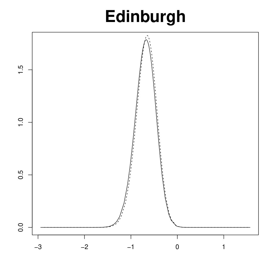 Figure 1
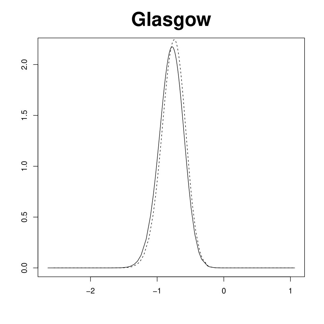 Figure 2
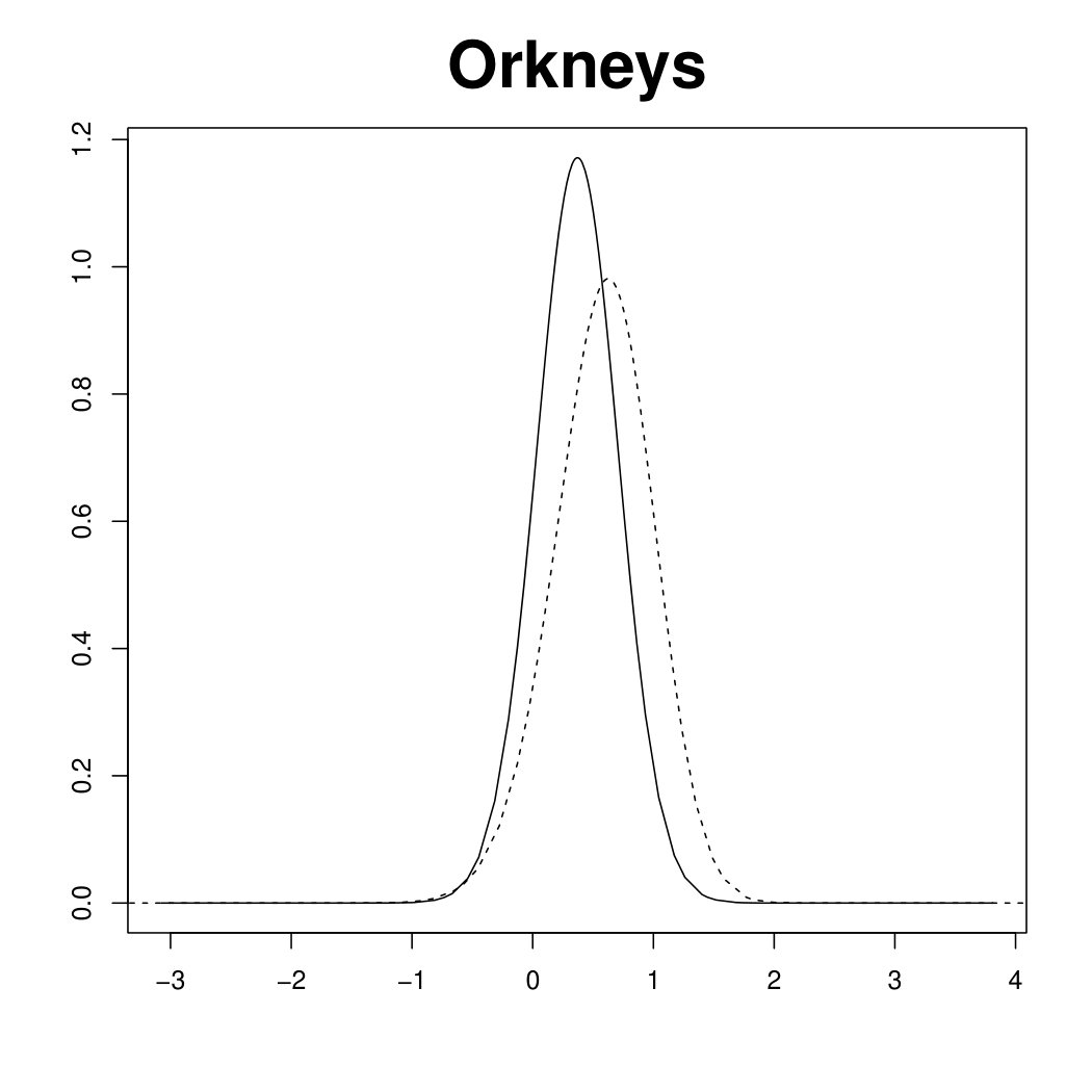 Figure 3
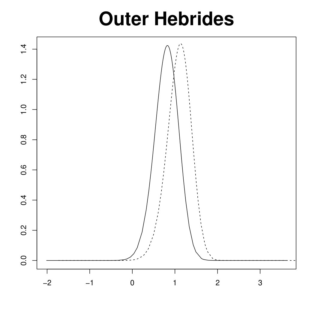 Figure 4
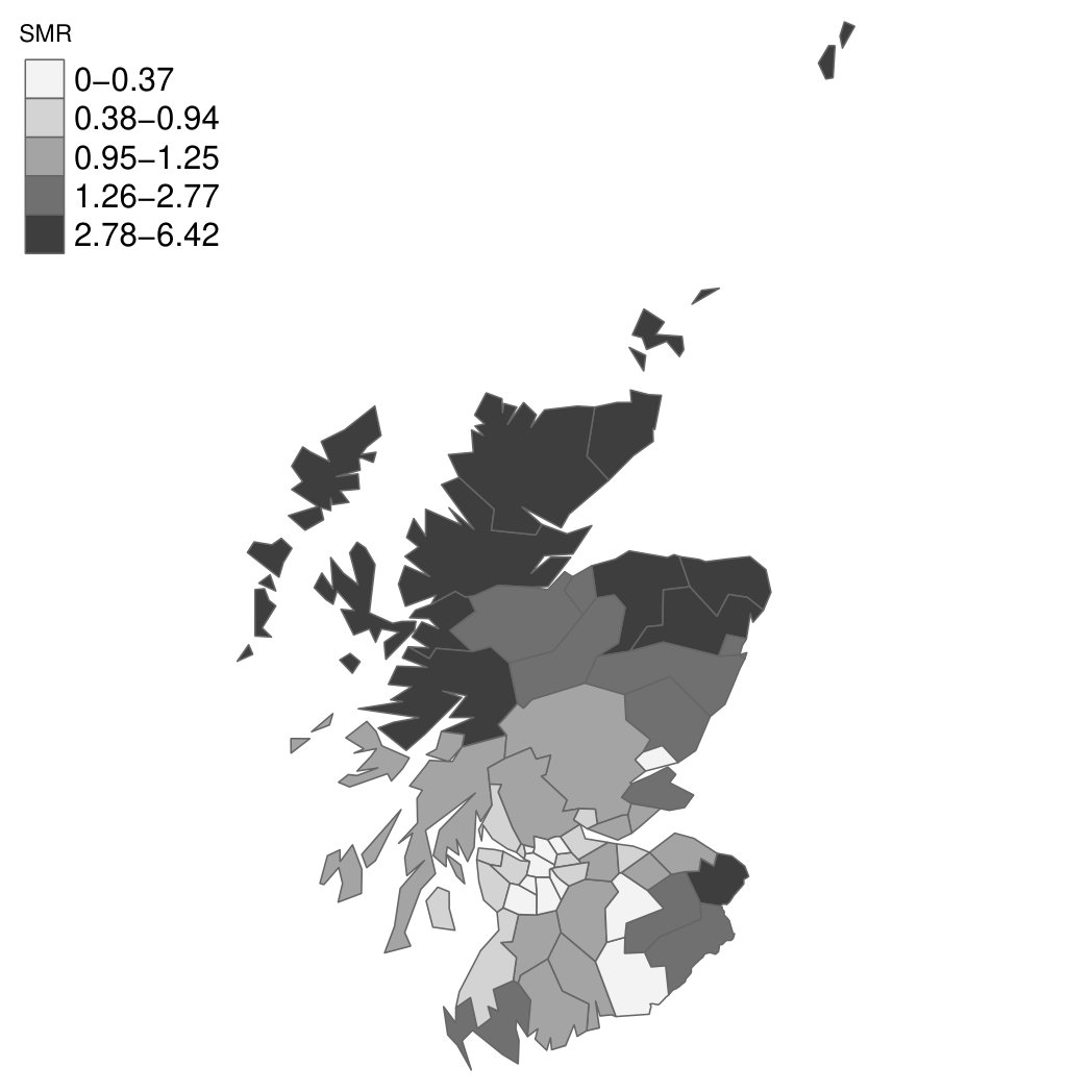 Figure 5
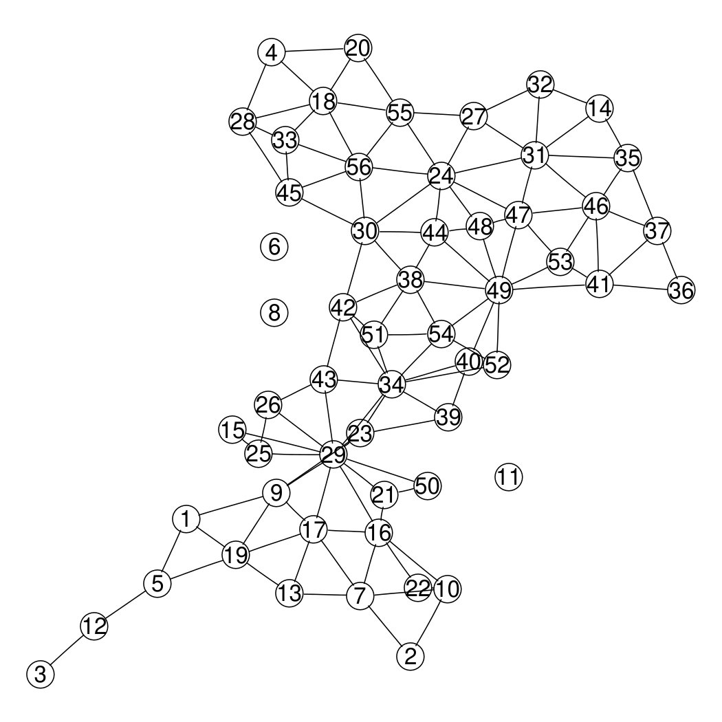 Figure 6
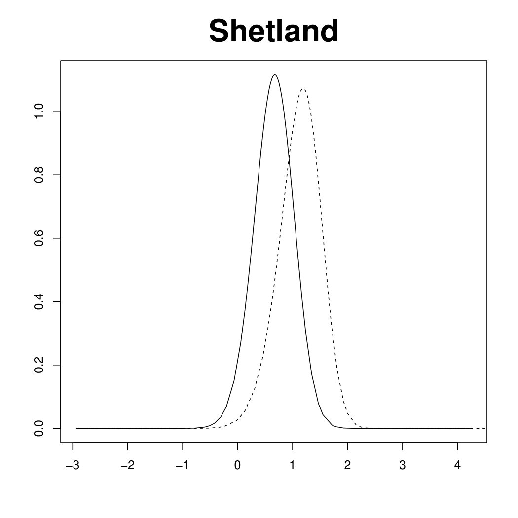 Figure 7
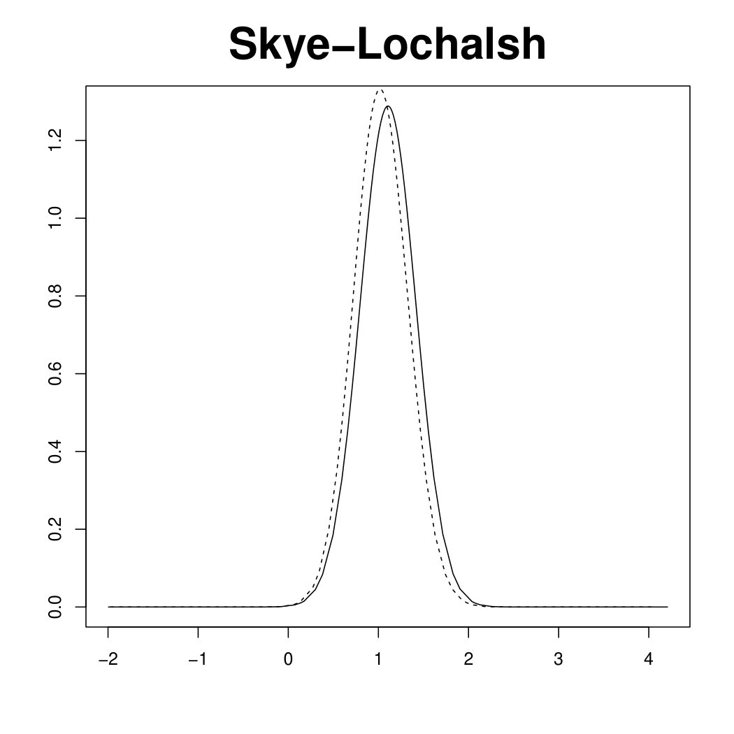 Figure 8
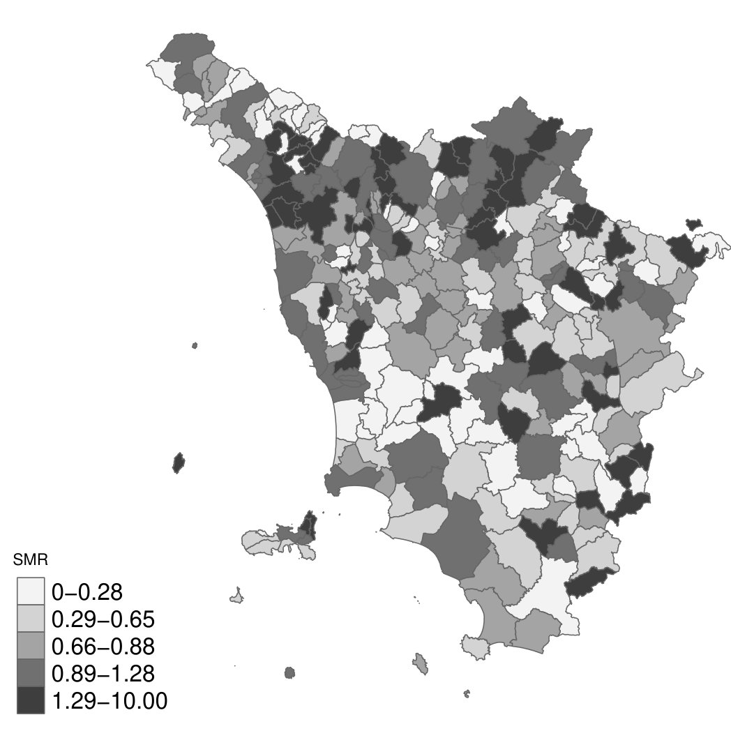 Figure 9
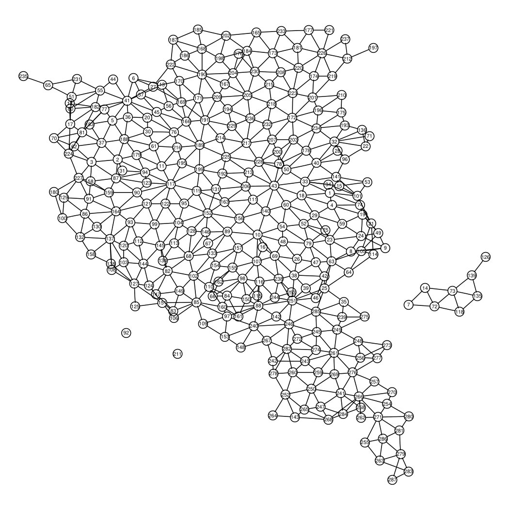 Figure 10
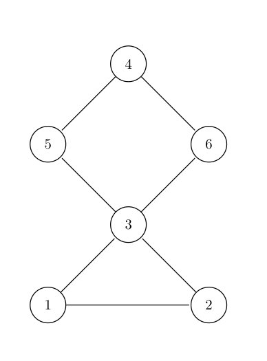 Figure 11
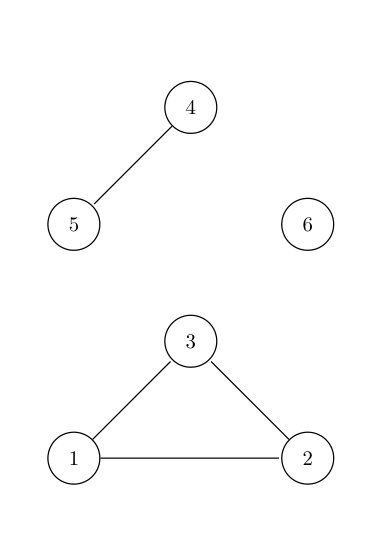 Figure 12
| Parameter | Mean | Standard | 2.5% | Median | 97.5% |
|---|---|---|---|---|---|
| deviation | |||||
| Scaled model | |||||
| (Marginal variance) | 3.97 | 1.17 | 2.16 | 3.81 | 6.69 |
| (Intercept) | -0.25 | 0.13 | -0.50 | -0.25 | -0.00 |
| (AFF) | 0.37 | 0.13 | 0.09 | 0.37 | 0.62 |
| (Orkneys) | 2.87 | 0.90 | 1.42 | 2.77 | 4.93 |
| (Shetland) | 2.06 | 0.73 | 0.95 | 1.95 | 3.80 |
| (Outer Hebrides) | 2.32 | 0.63 | 1.28 | 2.26 | 3.75 |
| Unscaled model | |||||
| (Marginal variance) | 2.26 | 0.70 | 1.18 | 2.15 | 3.91 |
| (Intercept) | -0.26 | 0.12 | -0.50 | -0.27 | -0.02 |
| (AFF) | 0.36 | 0.13 | 0.09 | 0.37 | 0.62 |
| (Orkneys) | 3.54 | 1.20 | 1.58 | 3.40 | 6.27 |
| (Shetland) | 3.26 | 1.18 | 1.36 | 3.11 | 5.96 |
| (Outer Hebrides) | 3.07 | 0.83 | 1.66 | 2.99 | 4.89 |
| Parameter | Mean | Standard | 2.5% | Median | 97.5% |
| deviation | |||||
| Prior for , | |||||
| (Intercept) | 1.12 | 0.06 | 0.99 | 1.12 | 1.24 |
| (Precision) | 1.31 | 0.22 | 0.93 | 1.30 | 1.79 |
| (Mixing parameter) | 0.24 | 0.12 | 0.06 | 0.22 | 0.54 |
| DIC | 1114.21 | ||||
| Prior for , | |||||
| (Intercept) | 1.126 | 0.06 | 1.00 | 1.124 | 1.128 |
| (Precision) | 1.38 | 0.22 | 0.99 | 1.37 | 1.87 |
| (Mixing parameter) | 0.26 | 0.13 | 0.06 | 0.22 | 0.52 |
| DIC | 1117.38 | ||||
Peer Reviews
No public reviews on file for this paper yet. If you reviewed it on a platform where reviews are public (OpenReview, ICLR, NeurIPS, ICML), you can paste yours below so the community can read it here.
Videos
No videos yet. Explain this paper in a talk, walkthrough, or lecture? Add one.
A note on intrinsic Conditional Autoregressive models for
disconnected graphs
Anna Freni-Sterrantino111Corresponding author, Small Area Health Statistics Unit, Department of Epidemiology and Biostatistics, Imperial College London, United Kingdom
Email:[email protected]
Massimo Ventrucci222Department of Statistics, University of Bologna, Bologna, Italy
Håvard Rue 333CEMSE Division, King Abdullah University of Science and Technology, Saudi Arabia
Abstract
In this note we discuss (Gaussian) intrinsic conditional autoregressive (CAR) models for disconnected graphs, with the aim of providing practical guidelines for how these models should be defined, scaled and implemented. We show how these suggestions can be implemented in two examples on disease mapping.
Keywords: CAR models, Disease mapping, Disconnected graph, Gaussian Markov Random Fields, Islands, INLA
1 Introduction
Conditional Autoregressive (CAR) models are widely used to represent local dependency between random variables. They are numerous applications in disease mapping [16, 5] and imaging [1]. In this paper, we introduce the specification of a CAR model on a disconnected graph and then show application on two disease mapping examples. To avoid unnecessary technicalities, we will throughout this note, only discuss a simple case, leaving the straightforward generalisation to the reader.
Disease mapping concerns the study of disease risk over a map of geographical regions. Let assume the study area is a lattice of non overlapping regions and is the number of cases of a given disease in region . For a rare disease, a Poisson model is assumed, , , with mean , where is the expected cases count for the disease under study (computed using the disease rates and demographic characteristics of a reference population) and is the relative risk, such that () means higher (lower) risk associated with living in region , while close to 1, indicates little difference between observed and expected in the region. The relative risk can be modelled in terms of the effect of a covariate , e.g. pollution, as , where and are respectively the baseline log risk and the effect of pollution. Value is a random effect capturing extra Poisson variability possibly due to unobserved risk factors.
When residual variability is spatially structured, a popular approach is to model the random effects with an intrinsic CAR, i.e. , . The precision hyper-parameter regulates the degree to which is shrunk to the local mean , which is the average of the random effects over its neighbours . This model is intrinsic in the sense that the overall mean is left unspecified and can be identified only when adding a linear constraint, such as .
On the applied side, this model is useful, for instance, when underlying population at risk is heterogeneous over the study area, with sometimes small expected counts in small regions. In these cases, the standardised incidence/mortality ratios are affected by large variances, hence a map of those ratios give a noisy representation of the disease risk over the study area. A CAR prior for the region-specific random effects ’s allows borrowing strength of information between neighbours, yielding a more reliable smooth map for the disease risk.
The definition of a CAR model starts by specifying a graph. A graph is a collection of nodes and edges representing, respectively, regions and neighbouring relationships between them. A graph is connected if there is a path (i.e. a set of contiguous edges) that connects each node to at least another node. Within a connected graph, specification of neighbouring relationships is clear (each node has at least one neighbour) and definition of a CAR model follows straightforwardly.
The specification of a CAR model on a disconnected graph is undefined and how should be carried out. There are essentially two types of disconnected graphs: first, a graph containing an island (a singleton node with no neighbours), second, a graph split in different sub-graphs (each of them being a connected graph).
In literature, there is a lack of attention [4] on the definition of a CAR for a disconnected graph, and/or on the properties of a CAR when the graph is disconnected. The only reference on this topic is Hodeges et al. [3] who discuss the form of the normalizing constant. One difficulty is how to deal with random effect in a singleton. GeoBUGS manual [15] offers some guidelines on this, with a default option which is to set to zero, if is a singleton. This practice is equivalent to enforce a sum-to-zero constraint on the singleton random effect: back to the disease mapping example, this automatically sets , if the baseline/covariate component is included in the model.
There are two issues with this approach. The first one is that it seems too restrictive, in the sense that even though a singleton random effect cannot capture spatially structured variability because it has no local mean to shrink to, should at least be allowed to model unstructured variability, hence shrinking towards a global mean. The second one and more general issue, with CAR models, regards scaling [14] which is important in order to interpret the prior assigned to the hyper-parameter . Care is needed when scaling the precision of a CAR model defined on a disconnected graph.
In the rest of this paper we discuss in detail the aforementioned two issues. In particular, in Sections 2 we define the intrinsic CAR model. In Section 3 and 4 we provide recommendations on appropriate scaling for the precision of a CAR model defined on connected and disconnected graphs, respectively. In Section 5 we give recommendations on linear constraints and discuss computation of the normalizing constant. In Section 6 we illustrate the proposed methods in two examples on disease mapping involving two different types of graphs. We conclude with a discussion in Section 7.
2 Intrinsic CAR models
In its simple form, the density of an intrinsic CAR model for is
[TABLE]
where is the set of all pair of neighbours, is a precision parameter, and is a normalising constant that we will return to later on. What qualify as a “neighbour” is application dependent and part of the model specification. For example, in many spatial applications, two regions ( and , say) are considered to be neighbours if they share a common border. The interpretation of (1) is that similarity between two neighbours are encouraged, and this induce a smoothing effect between neighbours, and thereby between neighbours of neighbours, and so on. We can formalize this, by defining a undirected graph , with a set of vertices , and the edges are the (unordered) set of neighbours. We then say that the intrinsic CAR is defined with respect to the graph .
The precision parameter determines the amount of smoothing and it is commonly estimated from data. The density (1) is improper or intrinsic, in the sense that is invariant to adding the same constant to all the ’s, as an example of a first order polynomial intrinsic CAR. Weighted and higher order polynomial (and non-polynomial) intrinsic CAR’s can be defined similarly; see [9, Ch. 3] for a thorough discussion.
We will focus on discussing the simplest case of an intrinsic CAR models for disconnected graph (1) to avoid technicalities which are discretional to understand the ideas, that are easily generalized to other types of intrinsic CAR models.
3 Scaling of an intrinsic CAR defined for a connected graph
Intrinsic CAR models has an unresolved issue with scaling, which is not immediate from studying (1). The basic reference is Sørbye SH et al.[14], which we will base our arguments in this section.
We will assume that the graph is connected, meaning that there is a path between all pair of nodes in the graph. An example of a connected graph is shown in Figure 1a.
The intrinsic CAR model (1) defined for this graph, has precision matrix
[TABLE]
The zeros are not shown. The intrinsic density is invariant for adding a constant to , meaning that and has the same improper density. However, what is of practical interest here, is how and how much this model varies around its mean value , i.e. how vary if we impose a sum-to-zero constraint . The critical issue is that this is a complicated function of the graph , for which we have no good intuition. For our example the (conditional on ) marginal variances are , , , , and for , which we interpret as follows.
The issue - that (conditional) marginal variances are different - is a feature of the intrinsic CAR model, and a consequence of that the conditional variance, , is inverse proportional to the number of neighbours of node (Eq.3.32[9]). 2. 2.
The ‘typical marginal variance’ is confounded with our interpretation of the precision parameter , and we do not know a-priori what means in terms of a typical marginal variance. In the Bayesian framework, this is crucial issue, since we need to impose a prior distribution for . We need to address what means in terms of its impact on the model.
The solution out of this appearently dilemma, is simply to scale so that the typical marginal variance is 1 when . Sørbye and Rue[14] recommend to use the geometric mean, which in our example, gives the following scaled precision matrix
[TABLE]
where . The most important consequence of this scaling, is that is now the typical precision and not only a precision parameter. This makes it possible to define a meaningful prior distribution and a clear interpretation for . There is a long tradition to prefer model parameters with a good and clear interpretation.
Our recommandation is clear and unambiguous.
Recommendation 1
We recommend to scale intrinsic CAR models defined with regard to connected graphs.
The scaling parameter can be computed as the geometric mean of the diagonal of the generalized inverse of when ; hereafter we denote as , if . However, this is not a computational efficient way to compute it has its an operation. A better approach, is to make use of the graph of the model and the knowledge of the null-space, and treat as a sparse matrix; see Rue and Held [9, Ch. 2.4] for background and details. The scaling can then be computed from a rank one correction of the marginal variances from the unconstrained model, see Rue et al.[10] for technical details about the recursions leading to the marginal variances. The computational cost will be be for typical spatial graphs, which is a huge improvement. The R-function inla.scale.model() in the R-INLA package (see www.r-inla.org) is an efficient implementation of this.
4 Scaling of an intrinsic CAR defined for a disconnected graph
A graph is disconnected if it is not connected. The practical interpretation of this related to (1), is that there are “islands” in the graph or nodes with no neighbours; we denote these nodes as singletons. Such cases easily appear if the graph is contructed from a map where we can have islands, or regions that are physically disconnected from the rest of the area. Figure 1b shows a disconnected graph with three connected components of size , and . We will use this graph as reference, in this section.
A direct application of the intrinsic CAR model for graph in Figure 1a, gives the precision matrix
[TABLE]
This matrix is singular with rank-deficiency of , since the density is invariant when we add a constant to each connected component. There are several unfortunate issues with this intrinsic CAR model, simply because the implicite assumption behind (1) is that the graph is connected. Additional to the issues discussed in Section 3, we have the following due to the disconnected graph.
- •
Node has no neighbours so and we have a constant density for . This can lead to an improper posterior distribution. To see this, consider the following model for an observed count, , in node ,
[TABLE]
where is the Poisson mean, , in logarithmic scale. The constant prior (5) implies an improper prior on the Poisson mean, i.e. . If a zero count is the case, then , which is improper. In other words, the constant prior for the singleton makes it difficult for the singleton random effect to shrink to the global mean. Also, this goes against the purpose of using (1) in the first place, which is to do smoothing and borrowing strength.
- •
The connected components for and are defined as on a connected graph. Even though this is reasonable within each connected components, it is not reasonable when we compare across connected components. As discussed in Section 3, the marginal deviation from its (component) mean, depends on the graph, and will in general be different for each connected component. In this simple case, the (conditional) marginal variance is constant within each connected component, and equal , and , respectively.
We can resolve both these issues by scaling (4) similar to what we did in Section 3, with two minor modifications.
We scale each connected component of size larger than one, independently as described in Section 3. 2. 2.
For connected components of size one, we replace it with a standard Gaussian with precision .
This scaling gives a well defined interpretation of and the same typical (conditional) marginal variance within each connected component, no matter the size. In our example, we obtain the following scaled precision matrix:
where and are the scaling values for the two connected components of size larger than one. Note, a normal prior with precision is assigned to the singleton in order for its marginal variance to be the same as for the nodes in the connected components. Our recommandation is clear and unambiguous. Therefore, due to the scaling, the precision parameter has the same interpretation for all sub-graphs, also for the singleton.
Recommendation 2
We recommend to scale intrinsic CAR models defined with regard to disconnected graphs.
5 Linear constraints and normalising constants
When using intrinsic models we always have to be careful not to introduce unwanted confounding. Let be the intrinsic CAR defined on a connected graph, then linear predictors and
[TABLE]
are the same. In the first case, there is no intercept as it is implicitly in the null-space of the precision matrix for . In the second case, we explicitly define the intercept and remove it from the intrinsic CAR model. We strongly prefer the second option, since it makes the interpretation of each component explicit and reduce the chance of misunderstanding and misspecifying the intrinsic CAR in more complex scenarios than here.
When the graph is disconnected, we designate one intercept for each connected component with size larger than one. Hence, we recommend to use one sum-to-zero constraint for each connected component of size larger than one. If one needs a connected component specific intercept, we prefer to add it to the model explicitly rather than implicitly.
Recommendation 3
We recommend to use a sum-to-zero constraint for each connected component of size larger than one.
Rue and Held [9, Ch 3] provide a strong case, to interpret the normalizing constant for the proper part of the model and the improper part as a diffuse Gaussian. Assume the graph has connected components, each of size . Then the normalizing constant for the scaled intrinsic CAR model (1), will be
[TABLE]
where
[TABLE]
and is a generalised determinant defined as the product of all non-zero eigenvalues. In most cases, we only need the part of that depends on , hence we do not need to compute the generalised determinant nor carry the around.
6 Application
In this section we provide two applications, in the first one we show how the scaling works with a disconnected graph, on lip cancer data from Scotland. In the second application, we want to give a broad picture of how scaling is related to the interpretation of the prior assigned to the precision parameter, using lung cancer mortality data for Tuscany Region (Italy).
6.1 Scottish Lip Cancer data: a graph with three singletons
The data are counts of lip cancer cases registered in 56 Scottish counties during years 1975-1980. We want to smooth the observed Standard mortality ratios (SMR), Figure 2a. We generate a graph by assuming the counties are the nodes, with edges connecting counties sharing borders, Figure 2b. Three counties are islands (Orkneys, Shetland and the Outer Hebrides), therefore we are left with three singletons in our graph. Breslow et al. [7] analyzed the spatial dependency using an intrinsic CAR model defined on a connected graph, obtained by editing new edges to connect the islands.
The popular WinBUGS software treats singletons as non-stochastic nodes and sets the associated random effects to zero by default (see GeoBUGS manual[15] page 18). From the perspective of developing user friendly software to fit Bayesian models via Markov Chain Monte Carlo (MCMC) algorithms this seems a safe strategy: if singletons are taken as stochastic nodes, with consequent improper , this may lead to poor mixing and extremely slow convergence especially when a zero count is observed; see the discussion in Section 4.
We argue that removing the singletons is needless for the definition of a suitable intrinsic CAR model. Our recommended solution is to avoid this and to assign the island-specific random effects a normal prior with zero mean and variance equal to [17].
Assuming vectors and are, respectively, observed and expected lip cancer cases during the study period, covariate is the “percentage of the population engaged in agriculture, fishing, or forestry”(AFF) and the unknown relative risks, the model is:
[TABLE]
In a direct application of the CAR model, the (unscaled) structure matrix in (8) contains the number of neighbours, , in position and values in positions , . If is a singleton, then and the prior for is constant. According to the recommendations in Section 4, we use the scaled version of (8), meaning that we scale the connected component of the graph of size larger than one (mainland) and assign a prior for each of the three singletons (islands). The scaling is coded in the inla.scale.model() function; in practice it is sufficient to flag as true the scale.model option when specifying the latent model in the package R-INLA [11, 6, 12] (see the code in the supplementary material Supplementary Material: INLA code to implement BYM2 models for disconnected graph)
The benefit of scaling is well illustrated by comparison against the unscaled version of the intrinsic CAR model. For the sake of comparison, for both scaled and unscaled models we assume a gamma with shape 1 and rate 5e-5 for the precision and apply a sum-to-zero constraint to the connected component of the graph (according to our recommendation given in Section 5).
Figure 3 displays the marginal posterior for six random effects fitted under the scaled (solid line) and unscaled (dashed line) model, using R-INLA. In the scaled model, the hyper-parameter has a clear interpretation as a typical precision. In other words, the (conditional) marginal variance within each of the four components of the Scotland graph (the mainland and the three singletons) is proportional to . In the unscaled model, the (conditional) marginal variances are different in each node of the graph. This issue is reflected in the large deviations in the top panels of Figure 3, referring to the three singletons (Orkneys, Shetland and Outer Hebrides). Note that the island-specific random effects, estimated by the unscaled model, are less shrunk towards no effect, , than those estimated by the scaled model. On the other hand, the posterior for the three random effects belonging to the connected component of the graph (bottom panels of Figure 3) are essentially unchanged between the two models. Results for the other nodes in the connected component are similar and not shown here. The different shrinkage properties of the scaled and unscaled models are confirmed by looking at posterior summaries for the main model parameters in Table 1. Though the fixed effects and are almost unchanged, the relative risks for the singletons are more extreme under the unscaled model than the scaled one.
6.2 Tuscany Lung cancer mortality: a graph split in
sub-graphs
In Section 1, we assert that the scaling plays an important role in the interpretation of the assigned prior on hyper-parameter , because it allows to have priors with the same interpretation on different underlying graphs.
In this second application, we want show the combination of the scaling and precision hyper-prameter priors, on an underlying disconnected graph. To show what we intend, we will introduce briefly a new parametrization for an intrinsic conditional autoregressive model and the concept of penalized complexity riors, see Simpson et al. [13]
Riebler et al. [8] defined an alternative Besag-York-Mollie (BYM) [1] parametrization, for the intrinsic conditional autoregressive, named bym2 (within R-INLA). The bym2 parametrization specifically accommodates scaling for connected or disconnected graph. In bym2, the random effect is , where is the spatially unstructured component and is the scaled spatially structured component (i.e. the scaled intrinsic CAR model).
The random effect is re-parametrized as
[TABLE]
with a covariance matrix
[TABLE]
The total variance is expressed by a mixing parameter () that measures the proportion of marginal variance due to the structural spatial effect. In addition, represents the precision of the marginal deviation from a constant level, without regard for any type of underlying graph. Finally, indicates the generalised inverse of the precision matrix. If the model is based solely on overdispersion, while if the model coincide with a Besag model: a pure structured spatial effect. Now, the specification of priors for and follows a penalized complexity priors approach (pc-priors). The pc-priors framework follows four principles: 1. Occam’s razor- simpler models should be preferred until there is evidence from more complex. 2. Measure of complexity- the Kullback-Leibler distance is used to measure increased complexity. 3. Constant rate of penalization- the deviation from simpler model has a constant decay rate. 4. User defined scaling- the user has a clear idea of a sensible size for parameters or on their transformations. Therefore, pc-priors are defined as informative priors that will penalize departure from a base-model. In this setting a base model presents a constant relative risk surface, therefore no spatial variation, opposed to a complex model, that shows spatial variation. The clarity gained by the pc-priors framework, allows the user to comprehensively state priors in terms of beliefs on and [8], where and are declared by choices of and in and , respectively. The two probabilities provide the user with an easy way to define an upper bound to what the user thinks as tail-event, and to assign an to this event it. The advantage of the pc-priors is the invariance to parametrization, that’s why they are very hand in situation with disconnected scaled graphs. We will show how these priors are declared and the results obtained, by using lung cancer deaths in women dataset (2585 total cases), collected for each municipality between 1981-1989, for the Tuscany Cancer Atlas. Tuscany presents two small islands, that have separate municipality and we will consider them as singletons - Capraia and Giglio Isles - and Elba Isle composed of 8 municipalities. In Figure 4a we plotted the standardised mortality ratio on Tuscany map, and the induced graphs composed of two major connected components and two singletons, Figure 4b. Note that SMRs are higher for northern municipalities and for Elba Island , where iron mine and steel mills were active since 1905 [2]. The SMR variance range is 0-100.
We fitted a Poisson regression without covariates and two pc-priors choices: the default values embedded in R-INLA(i), and then with some more informative priors values(ii). In the default setting has and , which assumes that the unstructured and structured random effects account equally to the total variability and has , a prior that corresponds to a marginal standard deviation for of and therefore to a residual relative risk smaller than 2, see Simpson et al. [13]. For our second choice, we specify , hence we assign a 95% to have a marginal standard deviation of . while maintaining ’s prior as default. For the choice of and is less intuitive than the mixing parameter, but is the marginal precision related to the residual relative risk. This means that we assign a 95% of having a residual relative risk smaller than .
In table 2, the intercept estimates stay unchanged, we see a slight change for the precision, while posterior marginal is supporting a major influence on non-spatial variability with a narrow credible interval, in both instances. Based on the Deviance Information Criterion (DIC) the first choice prior model is the one to prefer. However, as this can be seen as a sensitivity analysis, by twisting the precision prior we observed similar results. We are less concerned in this example with islands random effects, because we know that due to proper scaling they are shrank toward zero random effects.
7 Summary
We motivated the definition of intrinsic CAR models for disconnected graphs under two main recommendations: scaling the precision structure and applying sum-to-zero constraints on the connected components of the graph. Scaling the precision structure sets the typical marginal variance to ) in each component of the graph, where is the precision of the intrinsic CAR model. This immediately suggests a fair prior for random effects associated to the singletons in a disconnected graph in terms of a normal with zero mean and variance . The advantage is that the prior assigned to has the same interpretation regardless of the particular structure of the graph.
We applied this strategy to a disease mapping example on lip cancer in Scotland, using the natural disconnected graph with three island regions. In this example we emphasized overfitting of the unscaled model compared to the scaled one. In general, the extent to which the unscaled intinsic CAR leads to overfitting should depend on the structure of the graph, the sample size and the prior assigned to . When data contain little information about the disease risk for people living in the area (e.g. small regions with low expected counts, which is not the case with the lip cancer data), the prior may have large impact on the analysis. In this situations larger deviation between scaled and unscaled intrinsic CAR models must be expected, as the unscaled one has no control on the marginal variance, hence no control on the impact of , whereas the scaled one provides good intuition of .
In the second example we went further and combined the scaled strategy with an alternative parametrization and the application of informative priors (penalized complexity priors). We recommend always to use a scaled version for fitting disease mapping model for connected and disconnected graphs and we demonstrated that the modified BYM model (bym2) has clear and unambiguous parameter interpretation that are invariant to the underlying graph.
Supplementary Material:
INLA code to implement BYM2 models for disconnected graph
We show how to implement the model BYM2 for using R -package INLA, using data from Scotland lip cancer.
1 #Load the R-package
2library(INLA)
3
4*# load data*
5data(Scotland)
6
7*# show the first lines*
8head(Scotland)
9*# Counts E X Region*
10*#1 9 1.4 16 1*
11*#2 39 8.7 16 2*
12*#3 11 3.0 10 3*
13*#4 9 2.5 24 4*
14
15*# read the graph structure*
16graph.scot = system.file(”demodata/scotland.graph”, package=”INLA”)
17g = inla.read.graph(graph.scot)
18
19*# remove the edges to actually obtain the singletons,*
20*# these are nodes 6,8 and 11 (Orkneys, Shetland and*
21*# the Outer Hebrides)*
22id.singletons <- c(6,8,11)
23G<-inla.graph2matrix(g)
24G[id.singletons,]<-0
25G[,id.singletons]<-0
26
27*#generates the disconnected graph*
28g.disc <- inla.read.graph(G)
29
30
31*#sepcify the latent structure usig a fromula object*
32formula.bym2 = Counts~ 1+f(Region, model=’bym2’,
33 scale.model=TRUE,
34 adjust.for.con.comp=TRUE,
35 graph=g.disc,
36 hyper=list(
37 phi=list(
38 prior=’pc’,
39 param=c(0.5, 0.5)),
40 prec=list(
41 prior=’pc.prec’,
42 param=c(0.2/0.31,0.05),
43 initial=5)))
44*# call to the inla function*
45result= inla(formula.bym2, family=”poisson”, E=E, data=Scotland)
First we install the INLA package in R, with the command:
1install.packages(”INLA”,
2repos=”https://inla.r-inla-download.org/R/testing”)
In this paper we used INLA version0.0-1493893899 and we show the bym2 using Scotland data and graph, that are embedded in the package distribution. In line 2–8, we load the library and the Scotland data, and then inspect the first rows. The dataset is composed by four variables (line 9) : “Counts”- the number of lip cancer recorded; “E” the expected number of lip cancer; “X” the percentage of the population engaged in agriculture fishing or forestry and “Region” for the county. Then we read the graph associated with Scotland, lines 16–17. Because the graph is connected, we need to manually set the islands as singletons, lines 22-28. To do this we change the graph in to a matrix object and then we assign 0 in the respective positions, and re-transform the matrix in a graph.
In lines 32–43 we define the model structure in terms of an formula object. The f() function is used to specify the random effect in INLA. We specify the model in equation 9, by passing the as first argument the ”Region”, then declaring the model we are going to use, in this case bym2. We flag as true the options: scale.model to scale the graph and the adjust.for.con.comp to adjust for more than one connected component. We then provide the graph and in a list of arguments for the hyper parameters. In lines 37–39, we declare as a pc-prior and the two values for and . Similarly, in lines 40–42 we do the same for the precision parameter and in argument param we set first and then . The last argument of the hyper parameter list is initial that sets a value for the numerical optimisation start in INLA algorithm.
Finally we are ready to call function inla, with the formula, data and the likelihood. The object result can be inspected by typing summary(result) and plot(result), while posterior summaries are stored in resultssummary.random.
Acknowledgement
We thank Dr M. A. Vigotti (University of Pisa) for having made available the dataset from the Tuscany Atlas of Mortality 1971-1994. Massimo Ventrucci has been partially supported by the PRIN2015 (EphaStat) project founded by the Italian Ministry for Education, University and Research.
The reference list from the paper itself. Each links out to its DOI / PubMed record.
- 1[1] J. Besag, J. York, and A. Mollié. Bayesian image restoration with two applications in spatial statistics (with discussion). Annals of the Institute of Statistical Mathematics , 43(1):1–59, 1991.
- 2[2] A. Biggeri, D. Catelana, and E. Dreassia. The epidemic of lung cancer in tuscany (italy): A joint analysis of male and female mortality by birth cohort. Spatial and Spatio-temporal Epidemiology , 1(1)(31–40), 2009.
- 3[3] James S. Hodges, Bradley P. Carlin, and Qiao Fan. On the precision of the conditionally autoregressive prior in spatial models. Biometrics , 59(2):317–322, 2003.
- 4[4] L. Knorr-Held. Some remarks on gaussian markov random field models for disease mapping. In P. Green, N. Hjort, and S. Richardson, editors, Highly structured stochastic systems , pages 260–264. Oxford University Press, Oxford, 2002.
- 5[5] A. B. Lawson. Bayesian Disease Mapping: Hierarchical Modeling in Spatial Epidemiology . Chapman & Hall/CRC Interdisciplinary Statistics. Chapmann & Hall/CRC, 2nd edition, 2013.
- 6[6] T. G. Martins, D. Simpson, F. Lindgren, and H. Rue. Bayesian computing with INLA: New features. Computational Statistics & Data Analysis , 67:68–83, 2013.
- 7[7] D. G. Clayton N. E. Breslow. Approximate inference in generalized linear mixed models. Journal of the American Statistical Association , 88(421):9–25, 1993.
- 8[8] A. Riebler, S. H. Sørbye, D. Simpson, and H. Rue. An intuitive Bayesian spatial model for disease mapping that accounts for scaling. Statistical Methods in Medical Research , 25(4):1145–1165, 2016.