Some applications of Griffiths theorem in theory of Feynman integrals
Valentina A. Golubeva, Alexey N. Ivanov

TL;DR
This paper introduces a method leveraging Griffiths theorem to derive partial differential equations for Feynman integrals, including an algorithm for ladder diagrams, advancing computational techniques in quantum field theory.
Contribution
It presents a novel approach using Griffiths theorem to find PDEs for Feynman integrals and provides an algorithm specifically for ladder-type diagrams.
Findings
Developed a method to find PDEs for Feynman integrals using Griffiths theorem.
Created an algorithm for ladder diagram Feynman integrals.
Enhanced computational tools for analyzing Feynman diagrams.
Abstract
The present paper provides a method for finding partial differential equations satisfied by the Feynman integrals for diagrams of various types, using the Griffiths theorem on the reduction of poles of rational differential forms. As an application, an algorithm for computing partial differential equations satisfied by Feynman integrals for diagrams of a ladder type is described.
Click any figure to enlarge with its caption.
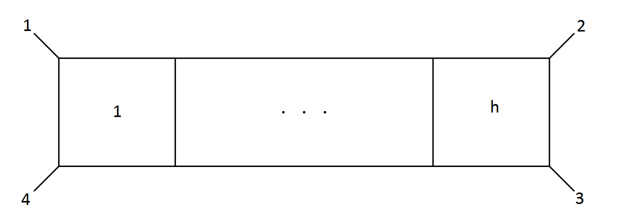 Figure 1
Peer Reviews
No public reviews on file for this paper yet. If you reviewed it on a platform where reviews are public (OpenReview, ICLR, NeurIPS, ICML), you can paste yours below so the community can read it here.
Videos
No videos yet. Explain this paper in a talk, walkthrough, or lecture? Add one.
Taxonomy
Topicsadvanced mathematical theories · Algebraic and Geometric Analysis · Polynomial and algebraic computation
Some applications of Griffiths theorem
in theory of Feynman integrals
Valentina A. Golubeva
Department of Applied Mathematics and Physics
Moscow Aviation Institute (National Research University)
4 Volokolamskoe shosse
125080 Moscow, Russia
and
Alexey N. Ivanov
Department of Mathematics
National Research University Higher School of Economics
6 Usacheva Street
119048 Moscow, Russia
Abstract.
The present paper provides a method for finding partial differential equations satisfied by the Feynman integrals for diagrams of various types, using the Griffiths theorem on the reduction of poles of rational differential forms. As an application, an algorithm for computing partial differential equations satisfied by Feynman integrals for diagrams of a ladder type is described.
Keywords: Feynman integrals, partial differential equations, Griffiths theorem
1. Introduction
Feynman integrals studied in the present paper enter the expressions for the elements of the -matrix in scattering problems of quantum field theory. To fix ideas, consider, for example, an initial state of a quantum system at the moment , characterized by some numbers of fermions and photons in specified individual states. The problem consists in describing the state of this system at the moment . The answer is given in terms of a wave function , that describes the states of the fields under consideration and satisfies the Schrödinger equation
[TABLE]
The general solution of this equation allows one to connect the values of the wave function at and by a transformation of the form
[TABLE]
The operator entering this expression is unitary and is called the scattering matrix (or the -matrix). The perturbation theory is the most widely known method for solving the scattering problem. The asymptotic series for the elements of the -matrix provided by the perturbation theory are sums of Feynman integrals corresponding to the Feynman diagrams with fixed number of internal lines.
The Feynman integrals of the quantum field theory are analytic functions with singularities, depending on certain physical parameters. The singularities occur along hypersurfaces, called singular varieties. The behavior of a Feynman integral in the neighborhood of its singular variety is similar to the behavior of hypergeometric functions. Analytical properties of Feynman integrals can be studied by various methods, for example, by means of series expansions near the singular variety (see [10]). These series expansions are derived from systems of partial differential equations for these integrals (see [1, 9]). In the present paper, we give a method for constructing such a system of partial differential equations for general Feynman integrals, based on the Griffiths theorem [5] on the reduction of poles of rational differential forms.
The structure of the paper is as follows. In Sec. 2, Feynman diagrams and parametric representations of Feynman integrals are defined. In Sec. 3, we introduce the necessary algebraic tools: the Griffiths Theorem and the Macaulay Theorem. In Sec. 4, we apply the Griffiths theorem to the problem of finding systems of partial differential equations for Feynman integrals corresponding to different types of diagrams (Theorems 1 and 2).
Acknowledgements. The work was supported in part by the Simons Foundation.
2. Parametric representations of Feynman integrals
Each term of the expansion of the -matrix in a series corresponds to some Feynman diagram. The Feynman diagram is a graph with lines topologically representing the propagation of elementary particles and vertices representing interactions of the elementary particles [2].
The graph consists of elements of two types, the lines and the vertices . There is the map sending each line to the pair of vertices , called the initial and final vertices of the line respectively. A line is incident with a vertex if it has this vertex as the initial or final vertex. A (minimal) loop of the graph is a sequence of lines such that , are incident with some vertex for each , while and are incident with some vertex , and the vertices are pairwise distinct. A loop can be formed by just one line. A path in the graph is a sequence of lines such that: 1) neither is a loop; 2) whenever ; 3) , are incident with a vertex ; 4) for . Denote by the vertex of , different from , and by the vertex of , different from . If the vertices are pairwise distinct, we will say that the path is simple. In this case the path starts at and end at . Denote by and the numbers of elements of the sets and , i. e. . If is the number of connected components of , then the number of independent loops of is . If several graphs are considered, then the above sets and numbers corresponding to a graph will be denoted by , .
A graph is called a Feynman diagram [3], if partitions of and of the following form are given:
[TABLE]
The vertices for are called external and the vertices for are called internal; the lines for are called massive and the lines for are called massless.
If is connected, then we denote by the graph which is obtained from by adding the infinity vertex that is connected with all external vertices by lines. Each line of a Feynman diagram is endowed with some orientation, but the Feynman integral defined below is independent of this orientation.
A subgraph of is a graph such that and . A subgraph of a graph is called a -tree if it contains no loops and if the number of its connected components is equal to . A spanning -tree of is a -tree which includes all the vertices of .
To each line of , one associates a parameter (these parameters are called the Feynman parameters). For every subset , we will write Define the polynomial , where the sum is taken over all spanning trees of . Let be an arbitrary subset of the set of external vertices of . Define another polynomial, W_{\chi}(\alpha)=\sideset{}{{}^{\prime}}{\sum}\limits_{T_{2}\subset G}\alpha(\Omega-T_{2}), where the sum is taken over all spanning 2-trees of such that its connected components contain subsets and respectively.
Let be a connected graph. Define the space of external momentum vectors satisfying the conservation law
[TABLE]
Assume that a symmetric bilinear form is given on whose quadratic form is positive definite when restricted to the real subspace of . So we can form the invariants
[TABLE]
from the external momentum vectors , where is a non-empty proper subset of the set . Due to the conservation law these invariants satisfy the relations
[TABLE]
[TABLE]
where are non-empty proper disjoint subsets of . If , then the relations (6), (7) are all the relations on the invariants that are consequences of their definition (5) (about the relations on the invariants for the case see [4]). Hence, we can fix a collection of subsets , such that all invariants are expressed in terms of , and these invariants are linearly independent (for example, \mathcal{X}=\big{\{}\{i\},\{j,k\}~{}|~{}i,j,k\in\Theta^{E}-{i_{0}}\big{\}}, where is some fixed external vertex).
So to each graph we can associate a set of complex parameters , which are the invariants defined above. Besides, to each internal line of , one associates a complex parameter called the squared mass for that line. Then the parametric representation of the Feynman integral for the given graph is defined by the following formula:
[TABLE]
where
[TABLE]
[TABLE]
and is a -dimensional piecewise smooth hypersurface lying in the first quadrant of the real subspace of such that its boundary lies on the coordinate hyperplanes . This hypersurface can be chosen in such a way that it does not intersect the variety .
3. Griffiths theorem on reduction of a pole of a rational differential form
Consider a rational differential -form on the projective space with homogeneous coordinates ,
[TABLE]
where and are homogeneous polynomials of degrees and in , such that . The form is a rational differential form with pole of order on the algebraic variety in . Below we will use the following Griffiths theorem on reduction of a pole of a rational differential form.
**Griffiths theorem [5]. ** Let be a rational differential -form on the projective space with pole of order on the variety , given by formula (11). If belongs to the ideal in the polynomial ring , generated by , i. e. if can be represented in the form , where are polynomials in and stands for , then there exists a rational differential -form , such that has a pole of order on the variety .
Proof. Assume belongs to the ideal , i. e. for some polynomials of degree . Consider the -form with pole of order on the variety :
[TABLE]
We have
[TABLE]
So we obtain
[TABLE]
It is necessary to note that under condition the exact differential form does not contribute to the integral by Stokes’ theorem, if the hypersurface satisfies the condition . Besides, the following theorem gives the condition under which belongs to the ideal.
**Macaulay Theorem [6]. ** Consider homogeneous polynomials on the projective space of degrees , such that the equations
[TABLE]
have no solution in . Then all the homogeneous polynomials of degree greater or equal to belong to the ideal .
We do not give a proof of this theorem. The proof consists in an application of the algorithm of constructing expansions of the form for polynomials from the ideal . Applying the Macaulay theorem to the homogeneous polynomials of degree , we see that any polynomial of degree belongs to the ideal provided .
4. Partial differential equations for some diagrams
Consider an arbitrary Feynman diagram and notice that for any homogeneous polynomial in variables of degree , we have the following formula:
[TABLE]
where , as before, denotes the number of independent loops, and .
**Theorem 1. ** The Feynman integral corresponding to an arbitrary Feynman diagram is a solution of the system of partial differential equations
[TABLE]
Proof. Consider the differential operator . According to (15) we have
[TABLE]
where . It is clear that belongs to the ideal generated by . Moreover, each polynomial in the expression is divisible by . So after applying the Griffiths theorem to the right hand side of (17), the contribution of the exact differential form (13) to the integral is zero. Hence, we have the following relation:
[TABLE]
On the other hand, according to (15) we have
[TABLE]
[TABLE]
Consequently, comparing the right hands of both previous identities we obtain the statement.
Recall that, for a given Feynman diagram, we have introduced a collection of subsets , such that all the invariants are expressed in terms of the invariants and the latter ones are linearly independent. Now assume that and consider the Feynman diagrams satisfying the following property:
(P) can be chosen in such a way that for all .
In other words, the corresponding polynomial (10) can be written in the form
[TABLE]
For example, the -loop ladder diagram (see the figure) and the one-loop -point diagram satisfy this property.
As above, notice that for any homogeneous polynomial in variables of degree we have the following equation:
[TABLE]
where W=\Big{(}W_{1},...,W_{r}\Big{)},\frac{\partial}{\partial s}=\left(\frac{\partial}{\partial s_{1}},...,\frac{\partial}{\partial s_{r}}\right).
**Theorem 2. ** Assume that the Feynman diagram satisfies the property (P). Then the corresponding Feynman integral is a solution of the system of partial differential equations
[TABLE]
for all such that the subset can be connected with the subset by an internal line .
Proof. Consider the differential operator . According to (16) we have
[TABLE]
where . It is clear that belongs to the ideal generated by . Moreover, due to the property (P), each polynomial is divisible by . So the polynomials in the expression are divisible by . Thus after applying the Griffiths’ theorem to the right hand side of (17) the exact differential form (13) gives no contribution to the integral. Hence, we have the following equality:
[TABLE]
On the other hand, according to (16) we have
[TABLE]
[TABLE]
Consequently, comparing the right hand sides of both previous identities, we obtain the statement.
Now we will present a general method for deriving partial differential equations of order on the example of a -loop ladder diagram. This method can be realized by using a computer algebra system.
Let \mathcal{X}=\big{\{}\chi_{1}=\{1\},...,\chi_{4}=\{4\},\chi_{5}=\{1,2\},\chi_{6}=\{2,3\}\big{\}}. Then the Feynman integral of the -loop ladder diagram has the following form:
[TABLE]
where , , . Consider the differential operators of order and respectively with undetermined coefficients depending on the parameters ,
[TABLE]
where we use the standard multi-index notation. According to (16) we have
[TABLE]
where the polynomials and have the following form:
[TABLE]
Next, consider the homogeneous polynomials of degree with undetermined coefficients and impose the following conditions on the polynomials :
[TABLE]
After collecting coefficients of appropriate monomials we obtain a system of homogeneous linear equations with unknowns Due to Griffiths theorem each solution of this system corresponds to a relation of the form , which is the wanted partial differential equation satisfied by the Feynman integral of a -loop ladder diagram.
The reference list from the paper itself. Each links out to its DOI / PubMed record.
- 1[1] V. A. Golubeva, Some problems in the analytic theory of Feynman integrals, Russian Mathematical Surveys (1976), 31(2):139.
- 2[2] N. Nakanishi, Graph theory and Feynman integrals, New York, Gordon and Breach, 1971.
- 3[3] E.R. Speer, M. J. Westwater, Generic Feynman Amplitudes, Ann. Inst. Henri Poincare 14: 1 (1971), 1 - 55.
- 4[4] E. Mihul, G. Gheorghe, n-point Lorentz-invariant distribution, preprint, Dubna, 1968.
- 5[5] P. A. Griffiths, On the periods of certain rational integrals, Ann. Math., Ser. 2, 90:3 (1969), 460-541.
- 6[6] F. S. Macauley, The algebraic theory of modular systems, London, Cambr. Univ. Press, 1916.
- 7[7] T. Gehrmann, E. Remiddi, Differential equations for two loop four point functions, Nucl.Phys. B 580, 2000, 485-518.
- 8[8] M. Argeri, P. Mastrolia, Feynman Diagrams and Differential Equations, Int.J.Mod.Phys. A 22, 2007, 4375-4436.