Cache-oblivious Matrix Multiplication for Exact Factorisation
Fatima K. Abu Salem, Mira Al Arab

TL;DR
This paper introduces a cache-oblivious matrix multiplication method using Morton-hybrid space-filling curves, significantly improving runtime for exact matrix factorization over finite fields.
Contribution
It develops a novel cache-oblivious approach for matrix multiplication tailored for parallel TU decomposition with Morton-hybrid layout, enhancing efficiency.
Findings
Orders of magnitude faster sequential evaluation
Low span in recursive matrix multiplication
Effective incorporation into parallel decomposition
Abstract
We present a cache-oblivious adaptation of matrix multiplication to be incorporated in the parallel TU decomposition for rectangular matrices over finite fields, based on the Morton-hybrid space-filling curve representation. To realise this, we introduce the concepts of alignment and containment of sub-matrices under the Morton-hybrid layout. We redesign the decompositions within the recursive matrix multiplication to force the base case to avoid all jumps in address space, at the expense of extra recursive matrix multiplication (MM) calls. We show that the resulting cache oblivious adaptation has low span, and our experiments demonstrate that its sequential evaluation order demonstrates orders of magnitude improvement in run-time, despite the recursion overhead.
Click any figure to enlarge with its caption.
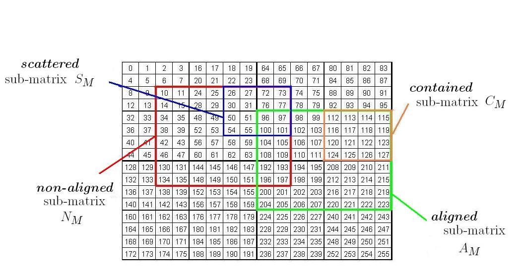 Figure 1
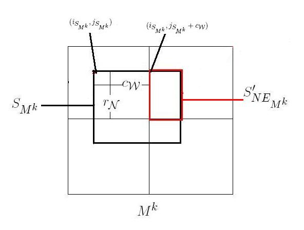 Figure 2
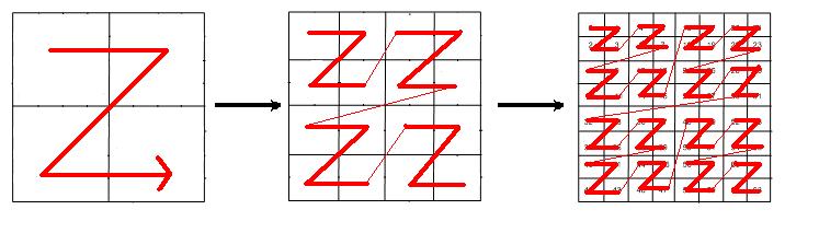 Figure 3
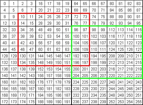 Figure 4
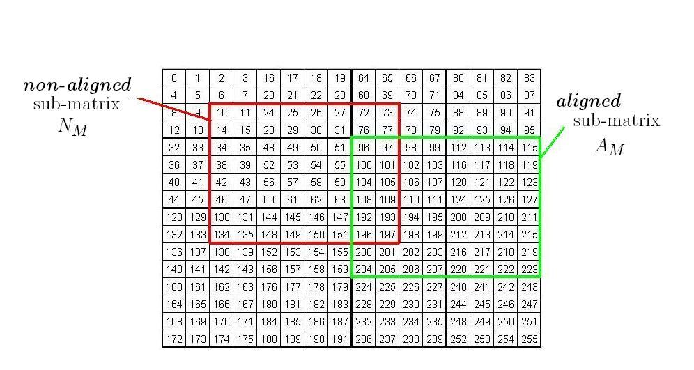 Figure 5
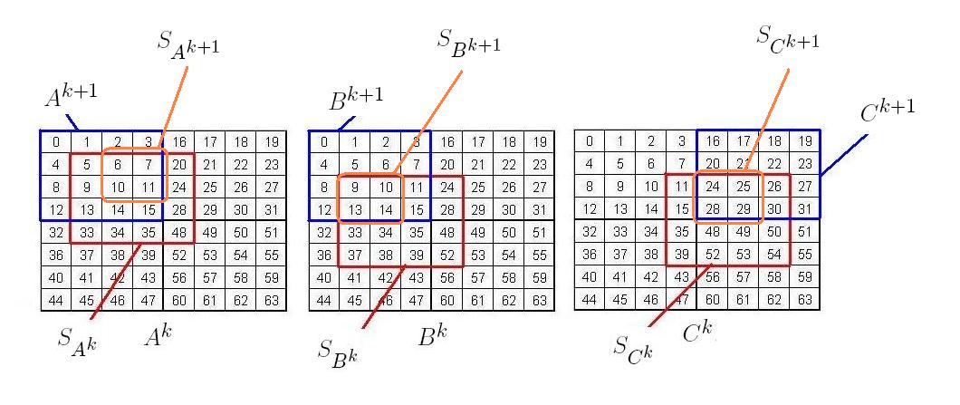 Figure 2
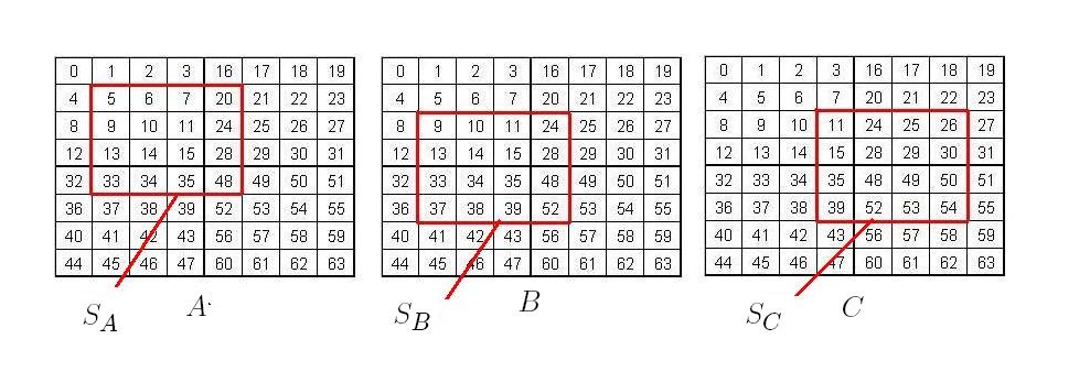 Figure 7
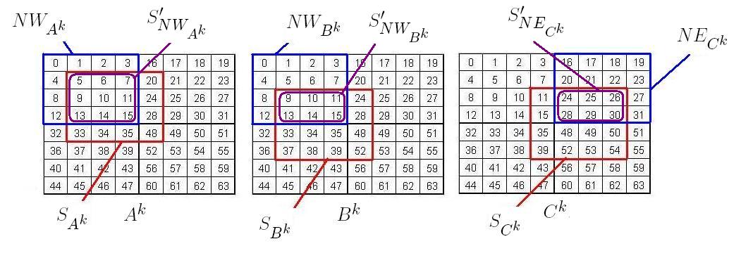 Figure 8
| % Inc. in Calls | % of Exp. | Avg. Imp. | Min. Imp. | Max. Imp. |
|---|---|---|---|---|
| 0 | 6.8 | 96.15 | 95.40 | 97.73 |
| 3.13 | 1.7 | 95.94 | 95.40 | 96.59 |
| 6.25 | 1.7 | 96.01 | 95.40 | 96.59 |
| 24.14 | 1.3 | 95.69 | 95.19 | 96.19 |
| 34.38 | 9.4 | 95.93 | 94.83 | 96.61 |
| 37.5 | 20.3 | 95.82 | 94.83 | 96.61 |
| 38.57 | 0.9 | 95.94 | 95.73 | 96.15 |
| 41.8 | 0.9 | 95.75 | 95.74 | 95.76 |
| 42.77 | 0.9 | 95.27 | 94.83 | 95.73 |
| 46.09 | 0.9 | 95.73 | 94.83 | 96.61 |
| 80.57 | 2.6 | 95.88 | 95.48 | 96.15 |
| 84.77 | 5.1 | 95.64 | 94.87 | 96.20 |
| 100 | 18.6 | 96.03 | 95.35 | 97.73 |
| 106.25 | 1.7 | 95.67 | 95.40 | 96.01 |
| 112.5 | 1.7 | 95.93 | 95.35 | 96.59 |
| 168.75 | 10.3 | 95.60 | 94.83 | 96.61 |
| 175 | 5.1 | 95.93 | 94.92 | 96.61 |
| 300 | 10.3 | 95.69 | 95.35 | 97.73 |
Peer Reviews
No public reviews on file for this paper yet. If you reviewed it on a platform where reviews are public (OpenReview, ICLR, NeurIPS, ICML), you can paste yours below so the community can read it here.
Videos
No videos yet. Explain this paper in a talk, walkthrough, or lecture? Add one.
Taxonomy
TopicsParallel Computing and Optimization Techniques · Advanced Data Storage Technologies · Cryptography and Residue Arithmetic
Cache-oblivious Matrix Multiplication for Exact Factorisation
Fatima K. Abu Salem111Corresponding author E-mail: [email protected]
Computer Science Department, American University of Beirut,
P. O. Box 11-0236, Riad El Solh, Beirut 1107 2020, Lebanon
Mira Al Arab 222E-mail: [email protected]
Computer Science Department, American University of Beirut,
P. O. Box 11-0236, Riad El Solh, Beirut 1107 2020, Lebanon
Abstract
We present a cache-oblivious adaptation of matrix multiplication to be incorporated in the parallel TU decomposition for rectangular matrices over finite fields, based on the Morton-hybrid space-filling curve representation. To realise this, we introduce the concepts of alignment and containment of sub-matrices under the Morton-hybrid layout. We redesign the decompositions within the recursive matrix multiplication to force the base case to avoid all jumps in address space, at the expense of extra recursive matrix multiplication (MM) calls. We show that the resulting cache oblivious adaptation has low span, and our experiments demonstrate that its sequential evaluation order demonstrates orders of magnitude improvement in run-time, despite the recursion overhead.
Keywords: Locality of reference, Cache-oblivious Algorithms, Space-filling Curves, Morton-hybrid Layout, TU Decomposition, Finite Fields
1 Introduction
We present a cache-oblivious adaptation of matrix multiplication to be incorporated in the paralel TU decomposition for rectangular matrices over finite fields, based on the Morton-hybrid space-filling curve representation. Exact triangulisation of matrices is crucial for a large range of problems in Computer Algebra and Algorithmic Number Theory, where a basis of the solution set of the associated linear system is required. Our focal algorithm of reference is the TURBO algorithm of Dumas et al. [7] for exact LU decomposition. This algorithm recurses on rectangular and potentially singular matrices. TURBO significantly reduces the volume of communication on distributed systems, and retains optimal work and linear span. TURBO can also compute the rank in an exact manner. As benchmarked against some of the most efficient current exact elimination algorithms in the literature, TURBO incurs low synchronisation costs and reduces the communication cost featured in [9, 10] by a factor of one third when used with only one level of recursion on 4 processors. A significant part of TURBO consists of matrix factorisation, and so, adapting this kernel in a cache-oblivious fashion will ultimately contribute to a cache oblivious factorisation algorithm. That TURBO has low depth makes adapting its sequential version to the cache-oblivious model more telling. Particularly, nested parallel algorithms for which the natural sequential execution has low cache complexity will also attain good cache complexity on parallel machines with private or shared caches [4].
At the base case of TURBO the sub-matrices reach a given threshold, and so one can take advantage of cache effects. To the best of our knowledge, no cache oblivious (or cache aware) algorithms for exact linear algebra exist in the literature. We pursue a cache oblivious adaptation using space-filling curves. TURBO requires index conversion routines from the space curve chosen and the cartesian order, due to the row and column permutations. In [1], using a detailed analysis of the number of bit operations required for index conversion, and filtering the cost of lookup tables that represent the recursive decomposition of the Hilbert curve, we have shown that the Morton-hybrid order incurs the least cost for index conversion routines as compared to the Hilbert, Peano, or Morton orders. The Morton order is the recursive -shaped space filling curve (Fig. LABEL:fig:fmorton_refinement). The Morton-hybrid order stops decomposing when the submatrices attain a threshold dimension [2]. At such a level, say when the submatrix fits in cache, the overhead for maintaining the curve representation outweighs the reduction in cache complexity. In reference to the literature cited in this manuscript around the Morton-order and its hybrid, this curve representation improves significantly on the temporal locality of various matrix algorithms such as naive multiplication, LU decomposition, and QR factorisation.
In this work, we introduce the concepts of alignment and containment of sub-matrices under the Morton-hybrid layout, and develop the full details of the MM algorithm by which it observes the alignment and containment of sub-matrices invariably across the matrix factorisation recursive steps. We do this by redesigning the decompositions within the recursive MM to force the base case to avoid all jumps in address space, at the expense of extra recursive MM calls. We show that the resulting cache oblivious adaptation retains optimal work and critical path length as default MM and thus is highly parallel. Our experiments confirm that the recursion overhead in the Morton-hybrid MM is negligible and leads to significant reduction in run-time thanks to its improved temporal locality.
Before proceeding, we begin with brief description of the TU algorithm. Consider a rectangular matrix over a field , where may be singular. is triangulated into the product of two matrices and , such that , where is a upper triangular matrix, and is with some “” patterns. This is done in a series of recursive steps on rectangular and potentially singular matrices, relaxing the condition for generating a strictly lower triangular matrix: (1) Recursive TU decomposition in SE, SW, NE, and NW (2) Virtual row and column permutations needed to re-order the blocks to yield the matrix . For brevity and because of lack of space, we omit the full details of the algorithm and refer the reader to [7] for a full account on TURBO.
2 Non-Aligned Rectangular Sub-matrix Multiplication Within The Recursion
Consider Morton-hybrid matrices , , and and let , , and be random sub-matrices of , , and respectively, for which one has to compute . This is a typical scenario encountered during the TU decomposition. To illustrate further, consider Fig. 7. Each integer appearing in the matrices in that figure represents the corresponding Morton-hybrid index of the element occupying it. The sub-matrices on which the multiplication is performed do not begin at the first entry of a Morton-hybrid sub-matrix, hence the concept of an aligned versus non-aligned Morton-hybrid sub-matrix.
An aligned sub-matrix is a sub-matrix of a Morton-hybrid matrix that begins at the first entry of a row-major sub-matrix. A non-aligned sub-matrix is a sub-matrix of a Morton-hybrid matrix that does not satisfy this condition.
Corollary 2.1
The Cartesian index of the first entry of an aligned sub-matrix is of the form , for any positive integers and .
Proof: By its definition, an aligned sub-matrix of a Morton-hybrid matrix starts at the first entry of some row-major sub-matrix of . Since the row-major sub-matrix is of dimensions , the Cartesian index of the first entry of is given by , for some positive integers and . By its definition, the aligned sub-matrix begins at an element of Cartesian index .
Corollary 2.2
If an aligned sub-matrix is , then it is row-major.
Proof: Let be a aligned sub-matrix of a Morton-hybrid matrix . From the definition of an aligned matrix, we know that begins at the first entry of a row-major sub-matrix of . According to the Morton-hybrid layout, all row-major sub-matrices of , including are . Since is also , then must be and hence is row-major.
An example of a non-aligned sub-matrix of a Morton-hybrid matrix with is shown in red in Fig. 7. An aligned sub-matrix is shown in green.
Next, we relate the lack of alignment of sub-matrices to the recursive accessing of these sub-matrices and discuss the implicated problems.
2.1 Non-Aligned Sub-Matrices and loss of locality
A sub-matrix of a Morton-hybrid matrix is said to be contained if lies completely within a sub-matrix of ordered in a row-major fashion. Otherwise, we say that is scattered.
Proposition 2.3
Let be an aligned sub-matrix of a Morton-hybrid matrix . The sub-matrix at the base case of the recursive division, down until sub-matrices, of is a row-major sub-matrix of .
Proof: First, we claim the recursive division of gives 4 aligned sub-matrices. From the definition of aligned sub-matrices, has size . So, the division of each of the dimensions of by 2 results in four quadrants , , , and of of size each. Thus these quadrants satisfy the size condition from the definition of aligned matrices. Note that once any of the dimensions reaches size it is no longer divided, and the recursive division proceeds on the other dimension until that too becomes . It is the size condition of this same definition that leads to sub-matrices at the base case of recursive division of the aligned sub-matrices decomposed from .
Now, recall, from Cor. 2.1, that the start index of is of the form . Then, the start indices of the sub-matrices resulting from the sub-division of are , , , and for the , , , and quadrants of respectively. Thus the start indices of these quadrants satisfy the start index condition from the definition of aligned matrices. Combining, by those two claims, the four quadrants resulting from the sub-division of any aligned matrix are aligned : they satisfy both conditions from the definition of aligned matrices.
Second, we show that the aligned sub-matrices at the base case are row-major sub-matrices of . If the recursive division continues till sub-matrices, we get aligned sub-matrices. From Cor. 2.2, we know that these sub-matrices are row-major sub-matrices of . This concludes the proof.
Corollary 2.4
Any sub-matrix of the sub-matrix reached at the base case of the recursive division of an aligned sub-matrix is contained.
Proof: According to Prop. 2.3, the sub-matrix at the base case of the recursive division of an aligned sub-matrix of a Morton-hybrid matrix is in row-major layout. Hence, any sub-matrix of this base case sub-matrix lies entirely within a row-major sub-matrix of and is therefore contained.
In Fig. 7, is one of the sub-matrices at the base case of the recursive division of the aligned sub-matrix and is a row-major sub-matrix. Any sub-matrix of is contained. When non-aligned sub-matrices are recursively divided, the sub-matrix at the base case may not consist entirely of a row-major sub-matrix of the Morton-hybrid matrix. It may be scattered across more than one row-major sub-matrix. For example, in Fig. 7, the sub-matrix is a sub-matrix at the base case of the recursion for the non-aligned sub-matrix in red. spans four row-major ordered sub-matrices - hence, it is scattered. We know that the elements of the sub-matrices at the base case are to be traversed in a row-major or column-major order, as required for the base case of MM. With such traversal imposed, a scattered sub-matrix suffers from two issues:
: Elements of a scattered sub-matrix are not sufficiently close in memory to maintain good spatial locality when traversed in a row/column-major fashion. This results in worse memory performance than for contained sub-matrices. 2. 2.
: Morton-hybrid encoding is required for accessing each element within a scattered sub-matrix (thus incurring extra computation overhead compared to row-major offset calculation).
Proposition 2.5
The loss in locality defined by and apply for scattered sub-matrices but not contained sub-matrices.
Proof: We first consider . Recall that the traversal of entries at the base case of the recursion is done in two orders: row-major and column-major. For contained sub-matrices, when consecutively accessing any two entries in any of these two orders, the minimum jump in address space is 1 and the maximum is as all entries lie within one row-major sub-matrix of the Morton-hybrid matrix. A scattered sub-matrix spans more than one row-major sub-matrix of the matrix. These row-major sub-matrices are not necessarily consecutive in memory and traversing, in a row-major or column-major fashion, the scattered sub-matrix that spans these row-major sub-matrices results in jumps in address space. When consecutively accessing any two entries of a scattered sub-matrix, the minimum jump in address space is 1 if the two entries being accessed consecutively belong to the same row-major sub-matrix and the maximum is for some positive integer , if the two entries belong to different row-major sub-matrices.
We now consider . Because the base case sub-matrix of an aligned sub-matrix is part of a row-major ordered sub-matrix, offset calculation for the elements at the base case is fast: traditional row-major offset calculation is used. Index of an element at offset from the start index of the sub-matrix at the base case is given by , since the sub-matrix satisfies a row-major ordering with row length = . This can be seen for the contained sub-matrix shown in Fig. 7 where . As for a non-aligned sub-matrix, accessing any element () in any of the base case sub-matrices requires that the corresponding Morton-hybrid index be calculated. This incurs extra calculation overhead as the encoding of the Morton-hybrid index is more costly than calculating an offset within a row-major ordered sub-matrix.
2.2 Modified Non-Aligned Sub-Matrix Multiplication
We aim to improve the sub-matrix multiplication procedure by addressing issues and . In this section, we describe a recursive sub-matrix multiplication algorithm which ensures that the sub-matrices at the base case of the recursion are contained in a row-major ordered sub-matrix of the original matrix. By doing this, we reduce the range of addresses of the elements within the sub-matrices at the base case as well as the number of jumps in address space done at the base case, and we eliminate the need for Morton-hybrid encoding at the base case. To ensure efficiency that the sub-matrix at the base case of MM is contained, by Prop. 2.3, the recursive division within the algorithm must start on aligned matrices. Recall the random matrices , , and in Morton-hybrid order and of dimensions , and , , and the random sub-matrices of , , and respectively (Fig. 7). We wish to perform the multiplication efficiently. We can recursively divide , , and , as in the default MM algorithm, which may result in scattered sub-matrices at the base case since , , and may not be aligned. Instead, we will recursively divide , , and and address only the relevant sub-matrix multiplications that ought to be done to produce . As , , and are aligned, recursively dividing them will enforce row-major sub-matrices at the base case from which we extract the relevant parts to produce .
Let be a superscript denoting a recursive step of the proposed MM algorithm. Also, let , , and , denote subscripts in (of sub-matrices of , , and respectively), indicating a specific quadrant following the Morton (Z-order): , , , and . For , , , and . Denote by , , and and the respective sub-matrices of , , and being multiplied as part of the overall multiplication . As such the initial problem is to produce . For this, we first produce the quadrants of , such that for . We do the same for and producing and respectively for . For each , we produce the sub-matrix, defined as the part of that lies in . Similarly, we produce , and . Note that is the two-dimensional concatenation of for and hence to calculate we need to calculate for . To do this, we need to consider all combinations of the form necessary to produce , as will be justified below. Now, when considering a combination , if the sub-matrices , , and are compatible for multiplication, i.e. the multiplication is part of the overall multiplication , then a recursive call is made on , , and . Else, if , , and are not compatible, we extract compatible parts of these sub-matrices and we label them as , , and on which the multiplication proceeds recursively. After doing this for all combinations for , we would have calculated .
We now describe the general ’th recursive step of Morton-hybrid MM, which consists of a round of four substeps. For simplicity, we drop the subscripts , and of , , and , and we use to denote any of the matrices , , or , Each aligned is identified by two values:
:
the Morton-hybrid index of the first element in the aligned matrix
:
the number of elements in the aligned sub-matrix
We are also given the sub-matrices of , of , and of on which we wish to perform the multiplication. Each of the sub-matrices is identified by the following:
:
the Morton-hybrid index of the first entry of
:
the number of rows of
:
the number of columns of
We do not use the 4-tuple to identify the aligned sub-matrices because the 3-tuple simplifies the computations for identification of the quadrants of and incorporates the information from the 4-tuple where and .
Step 1: In this step, we need to identify all four aligned quadrants , , of the aligned , for not reaching the base case, to proceed with the recursive multiplication algorithm. The index is dropped from for simplicity. To do this, we identify the start index and size of each quadrant of . Because is divided into four quadrants of equal size, the number of elements in any quadrant is given by . Recall, that in the Morton-hybrid order, the quadrants not reaching the base case are stored according to the Morton layout. For the Morton order, the quadrants of are laid out in the order , , , then , and hence
- •
- •
- •
- •
The sub-matrix may not lie entirely within one quadrant of and hence all quadrants of which contain part of must be considered, which is the case in the example from Fig. 7 as , , and touch on all four quadrants of , , and respectively. Given , we must now identify, for each , the part of that lies within . We denote this sub-matrix by . The method to identify now follows.
Step 2: Recall that we are given and as input into the recursion. As may not lie entirely within one quadrant of , it is scattered, and we must identify the parts of which lie in denoted by . We have identified the quadrants , for , and now we will identify the part of that lies within each , denoted by . Then is the two-dimensional concatenation of for . Here we drop the index for simplicity. To identify , we need to identify its start index and dimensions . To do this, the following intermediate values are needed. For simplicity, the indices of the intermediate values denoting dependence on are omitted.
:
The number of rows of in , the northern half of .
:
The number of columns of in , the western half of .
:
The number of rows of in , the southern half of .
:
The number of columns of in , the eastern half of .
:
The Morton-hybrid index of the last entry of . Similarly for , , and .
:
Given an entry of Cartesian index , returns the Morton-hybrid index of
:
Given an entry of Morton-hybrid index , returns the coordinate of the Cartesian index of
:
Given an entry of Morton-hybrid index , returns the coordinate of the Cartesian index of
The identification of is done as follows:
- •
For , calculate as follows:
[TABLE]
and, for , use
[TABLE]
- •
Find using , i.e. is the difference between the row indices of the last entry of and the first entry of and represents the number of rows of in the northern half of . Similarly, we find
[TABLE]
the number of columns of in the western half of . Note that if then no part of lies in the north half of and if then no part of lies in the west half of . After finding and , we can find and using and , which are the remaining rows and columns of respectively
- •
So far, we have found the number of rows in the northern and southern halves of and the number of columns in the western and eastern halves of and we want to identify , , and for each . Recall that we are able to identify a sub-matrix by a 4-tuple , where is the Morton-hybrid index of the first entry of the sub-matrix and and are its row and column dimensions respectively. Let denote the Cartesian index of the first entry of found using and . We now identify , , and according to the following cases:
For , , , and . 2. 2.
For , , , and . 3. 3.
For , , , and . 4. 4.
For , , , and .
To justify these cases we will explain how we arrived at case 2 for example where we identify the start index and dimensions of as shown in Fig. 7. The rest follow similarly. Recall that denotes the Morton-hybrid index of the first element of , and that is the corresponding Cartesian index. The index is the Cartesian index of the first element in . The corresponding Morton-hybrid index can be found using the function . The dimensions of are .
Note that for each , the Cartesian index of the start entry of Morton-hybrid index is given by , for and .
Step 3: By now we have decomposed each into quadrants, and we have identified, for each quadrant , the part of within that quadrant denoted by . The matrix is the two-dimensional concatenation of for . Next, we identify which quadrants , , and to consider for recursive multiplication. For each quadrant of , we have identified (same for for and , for all ). We need to perform the multiplications within and required to calculate . As an example, examine from Fig. 7. The sub-matrix is given by the 4-tuple . We identify this tuple using Step 2 above. To calculate of , the sub-matrix from given by is to be multiplied by the sub-matrix from given by . According to our approach, this will be done in a way so as to ensure that the sub-matrices being multiplied at the base case are contained , which improves locality and reduces conversion overhead as described earlier. Because the sub-matrices and of and touch on all four quadrants of and , and we want to calculate , all quadrants of are to be considered for multiplication with all quadrants of . Those are given by the following sixteen combinations of quadrants from and :
[TABLE]
All of these are needed to calculate . But, to calculate the sub-matrix , we need to find , , and in addition to because is the two-dimensional concatenation of for . Similarly as above, to determine each of these quadrants of requires sixteen combinations of quadrants from and . In total, to find , we would need up to sixty-four combinations of quadrants from , , and .
Step 4: For each combination, if , , and are not compatible, we extract compatible parts of these sub-matrices and we label them as , , and on which the multiplication proceeds recursively. How to extract compatible parts is beyond the scope of the present manuscript and is left for future work 333We also note that omiting this part of the algorithm does not deflect from its main rationale.. For now, we concede that omiting it does not divert from the general understanding of the overall algorithm, and that the work requirements for this step can be embedded in that required to perform Steps 1 –¿ 3 above.
Proposition 2.6
If using auxiliary space to peform the matrix additions, and assuming the matrix is of dimensions at most , where is the machine word-size, the cache oblivious MM using Morton-hybrid order requires asymptotically the same work and critical path lenth as default MM.
Proof: On work: The cache-oblivious algorithm is a divide and conquer algorithm. The divide phase introduces two new functions over the default MM algorithm consisting of Steps 1 and 2 above. Each of these steps requires a constant number of arithmetic operations and calls to encoding and extraction procedures. From Sec. 3.5 of [1], we know that each encoding or extraction procedure incurs a constant number of operations assuming the matrix is of dimensions at most , where is the machine word-size. For the typical value , such matrix sizes are sufficiently large for many applications. It follows that the work of the cache-oblivious algorithm is asymptotically the work of the default algorithm given by . The conquer part creates non-overlapping sub-problems in Steps 3 and 4 above whose union yields the original matrix to be multipled.
On parallelism: All of the extra 64 recursive calls are independent and thus can be cast in parallel. If auxiliary space is available to perform the matrix additions required for each MM, one can also perform addition in parallel using the standard algorithm (Ch. 27 of [6]). Hence, the critical path length of the cache-oblivious algorithm remains that of the default multithreaded algorithm and is known to be .
Remarks on implications for Parallel Performance: The sub-matrices at the base case of the recursion are contained within a row-major sub-matrix, thanks to enforcing aligned sub-matrices for the recursive division. The Morton-hybrid, cache-oblvious version demonstrates superior performance over the default algorithm, and eliminates the need for Morton-hybrid index conversion when accessing each element in the sub-matrix at the base case, as it can proceed instead with row-major encoding. The implications for parallel performance can be captured using the results from [4], which reveal that nested parallel algorithms for which the natural sequential execution has low cache complexity will also attain good cache complexity on parallel machines with private or shared caches. In this framework, our adaptation combines improved temporal locality using the Morton-hybrid order for the serial algorithm as well as optimal work and critical path length for the multithreaded version.
Performance Analysis We now verify that the cost of increased recursive MM calls for the cache-oblivious sub-matrix multiplication is significantly compensated for by the improvement in temproal locality thanks to the Morton-hybrid order. We use a Pentium IV of 2.8 GHz processor speed, with an 8 KB L1 cache and a 512 KB L2 cache. It runs linux version 2.6.11 and gcc compiler version 4.0.0. We generate random Morton-hybrid matrices and multiply random sub-matrices of these matrices using both the default and cache-oblivious algorithms. To neutralise the effect of modular aritmetic over finite fields and to be able to exclusively account for the gains induced by the Morton-hybrid order, the random matrices we generate are taken over the binary field. According to [3], is the typical value for the truncation size for block recursive matrix algorithms of floating point entries that shows improvements in cache misses and cycles for Morton-hybrid, default MM. Recall the multiplication of rectangular sub-matrices , where , and are square and in Morton-hybrid order. The dimensions of the square matrices are of no significance, since the multiplication kernel is operating on the rectangular sub-matrices. We thus partition Morton-hybrid matrices of dimensions and multiply sub-matrices of these Morton-hybrid matrices of varying sizes. Each experiment is distinguished using varying indices of the starting entries of each and varying dimensions and . Because of the variation in sizes across each experiment we do not report on the run-times of each but rather choose to report on the percentage of increase, or decrease, in the number of base case calls made by the cache-oblivious over the default algorithm and the associated percentage of improvement. We record the number of recursive MM calls made to the base case of each of the two algorithms and the total time taken by the overall multiplication to finish. The results are presented in Table 1. We interpret it using the fifth row, say, as an arbitrary example. Of all 468 experiments run in total, about 9% of them exhibited about 34% increase in recursive calls made by the cache-oblivious over the default algorithm. The average, maximum, and minimum percentages of improvement in run-time across this batch of experiments is shown thereafter, and are all staggeringly high. Examining all rows, one can see that no matter what the increase in MM recursive calls has been, this hardly affects the high percentages of improvement. The reductions in cache misses as a result of the cache-oblivious algorithm overwhelm the cost to handle extra recursive calls.
The reference list from the paper itself. Each links out to its DOI / PubMed record.
- 1[1] F. K. Abu Salem and M. Al Arab. “Comparative study of space filling curves for cache oblivious TU Decomposition”, extended report, http://arxiv.org/abs/1612.06069
- 2[2] M. D. Adams and D. S. Wise. “Fast additions on masked integers”, in SIGPLAN Not. , 41(5):39–45, 2006.
- 3[3] M. D. Adams and D. S. Wise. “Seven at one stroke: results from a cache-oblivious paradigm for scalable matrix algorithms”, in MSPC ’06 ,41–50, ACM Press, 2006.
- 4[4] G. Blelloch, P. B. Gibbons, and H.-V. Simhadri. “Low depth cache-oblivious algorithms”, in SPAA 2010 , pp. 189-199, ACM Press, 2010.
- 5[5] N. Chen, N. Wang, and B. Shi. “A new algorithm for encoding and decoding the hilbert order”, in Softw. Pract. Exper. , 37(8):897–908, 2007.
- 6[6] T. H. Cormen, C. E. Leiserson, R. L. Rivest and C. Stein. Introduction to Algorithms, 3rd edition, MIT Press.
- 7[7] J.G. Dumas and J.L. Roche. “A parallel block algorithm for the exact triangulization of rectangular matrices”, in SPAA 2001 , pp. 324-325, ACM Press, 2001.
- 8[8] Jeremy D. Frens and David S. Wise. “QR factorization with Morton-ordered quadtree matrices for memory re-use and parallelism”, in P Po PP ’03 , pp. 144–154, ACM Press, 2003.