Exact short-time height distribution in 1D KPZ equation with Brownian initial condition
Alexandre Krajenbrink, Pierre Le Doussal

TL;DR
This paper derives exact short-time height distribution formulas for the 1D KPZ equation with Brownian initial conditions, revealing detailed large deviation behaviors and phase transition features.
Contribution
It provides the first exact expressions for the rate function of the KPZ height distribution with Brownian initial conditions, connecting to weak noise theory and symmetry breaking phenomena.
Findings
Exact rate function $\Phi(H)$ for $H<H_{c2}$ derived.
Identified phase transition point $H_{c2}$ with symmetry breaking.
Asymmetric tails with $|H|^{5/2}$ and $H^{3/2}$ behavior.
Abstract
The early time regime of the Kardar-Parisi-Zhang (KPZ) equation in dimension, starting from a Brownian initial condition with a drift , is studied using the exact Fredholm determinant representation. For large drift we recover the exact results for the droplet initial condition, whereas a vanishingly small drift describes the stationary KPZ case, recently studied by weak noise theory (WNT). We show that for short time , the probability distribution of the height at a given point takes the large deviation form . We obtain the exact expressions for the rate function for . Our exact expression for numerically coincides with the value at which WNT was found to exhibit a spontaneous reflection symmetry breaking. We propose two continuations for , which apparently correspond to…
Click any figure to enlarge with its caption.
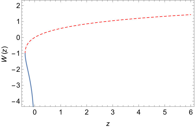 Figure 1
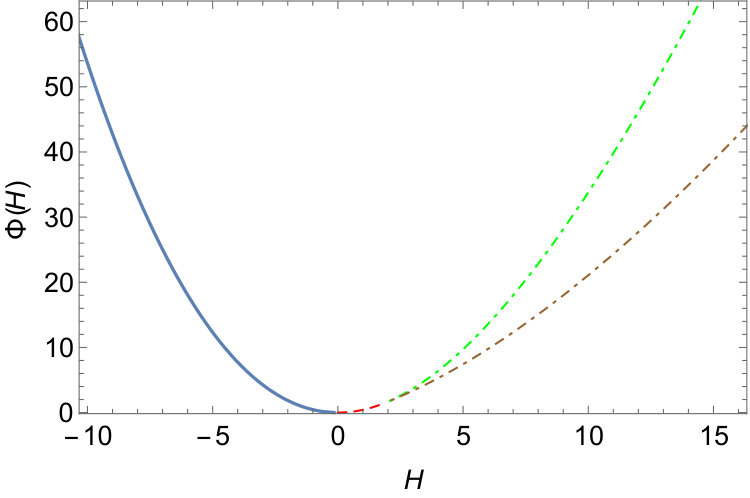 Figure 2
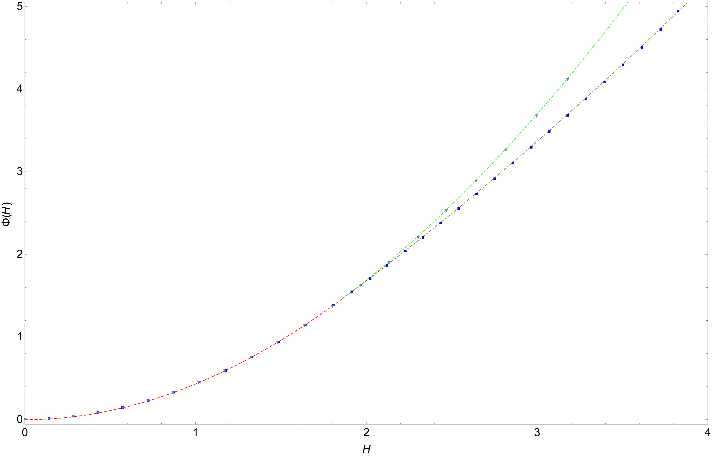 Figure 3
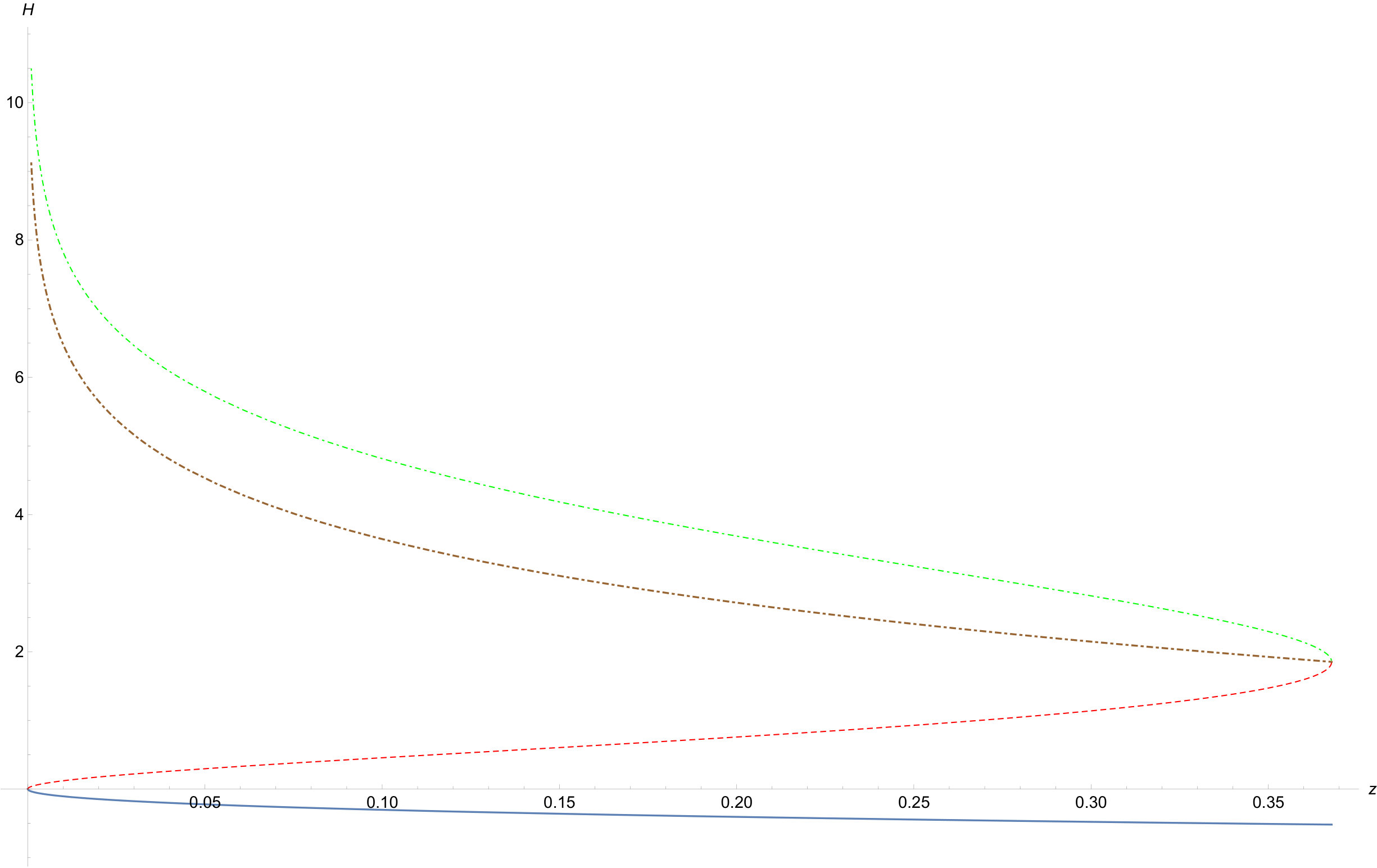 Figure 4
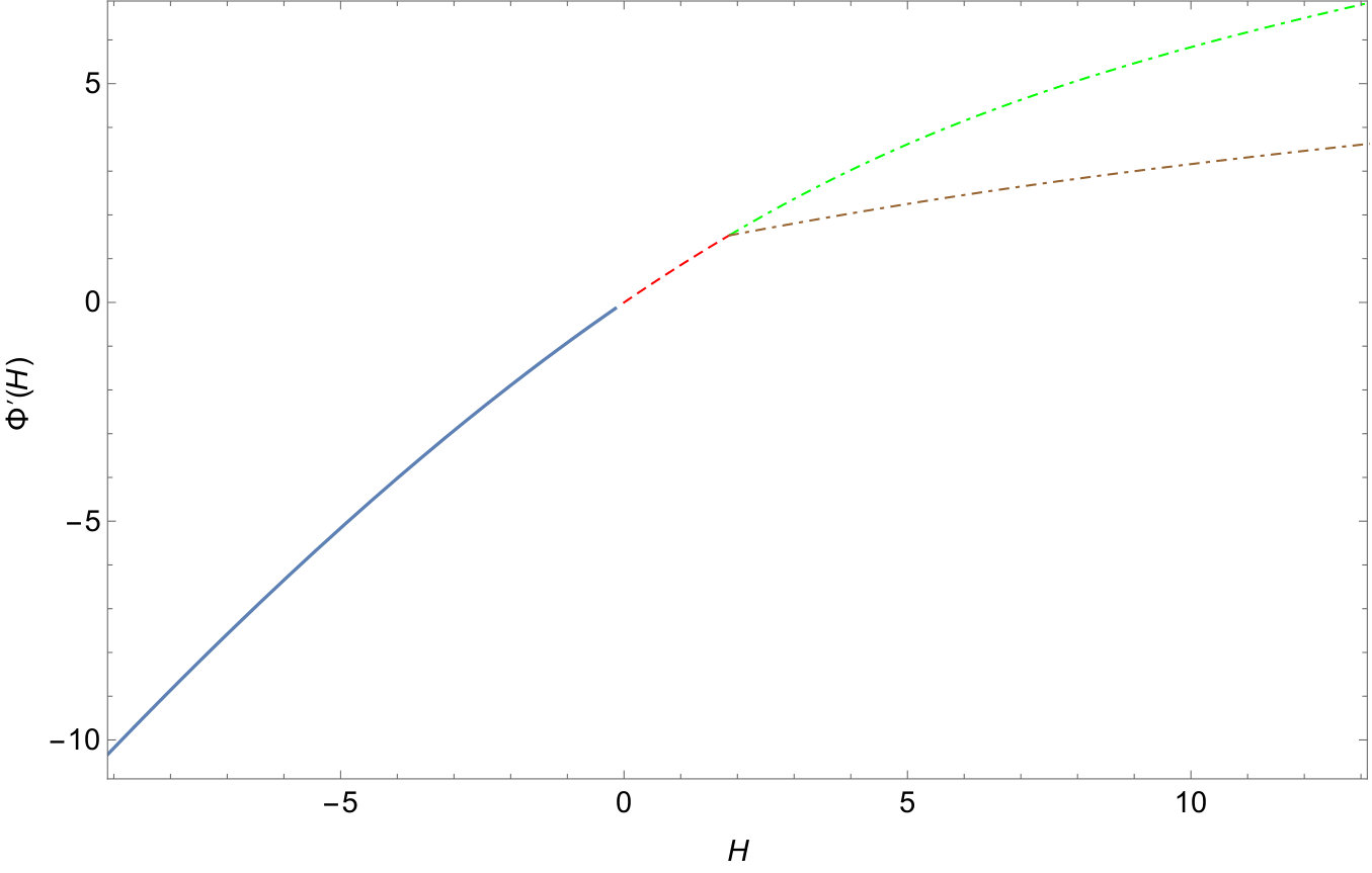 Figure 5
 Figure 6
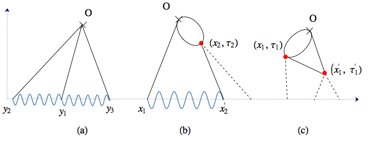 Figure 7
Peer Reviews
No public reviews on file for this paper yet. If you reviewed it on a platform where reviews are public (OpenReview, ICLR, NeurIPS, ICML), you can paste yours below so the community can read it here.
Videos
No videos yet. Explain this paper in a talk, walkthrough, or lecture? Add one.
Exact short-time height distribution in 1D KPZ equation with Brownian initial condition
Alexandre Krajenbrink
CNRS-Laboratoire de Physique Théorique de l’Ecole Normale Supérieure, 24 rue Lhomond, 75231 Paris Cedex, France
Pierre Le Doussal
CNRS-Laboratoire de Physique Théorique de l’Ecole Normale Supérieure, 24 rue Lhomond, 75231 Paris Cedex, France
(March 7, 2024)
Abstract
The early time regime of the Kardar-Parisi-Zhang (KPZ) equation in dimension, starting from a Brownian initial condition with a drift , is studied using the exact Fredholm determinant representation. For large drift we recover the exact results for the droplet initial condition, whereas a vanishingly small drift describes the stationary KPZ case, recently studied by weak noise theory (WNT). We show that for short time , the probability distribution of the height at a given point takes the large deviation form . We obtain the exact expressions for the rate function for . Our exact expression for numerically coincides with the value at which WNT was found to exhibit a spontaneous reflection symmetry breaking. We propose two continuations for , which apparently correspond to the symmetric and asymmetric WNT solutions. The rate function is Gaussian in the center, while it has asymmetric tails, on the negative side and on the positive side.
pacs:
05.40.-a, 02.10.Yn, 02.50.-r
Many works have been devoted to studying the 1D continuum KPZ equation KPZ ; directedpoly ; reviewCorwin ; HairerSolvingKPZ , which describes the stochastic growth of an interface of height at point and time as
[TABLE]
starting from a given initial condition . Here is a centered Gaussian white noise with , and we use from now on units of space, time and heights such that and SuppMat . A lot of the interest in (1) is motivated by the broad universality class of models johansson ; baik2000 ; spohn2000 ; corwinsmallreview ; reviewSpohn2015 and experimental systems HH-TakeuchiReview ; myllys ; PLDKaz2times , which share the same asymptotic scaling behavior of their height fluctuations. It has focused mainly on the limit of large time, for which the universal Tracy-Widom distributions TWAll have been found to emerge CLR10 ; DOT10 ; SS10 ; ACQ11 ; PLDflat .
Recently, the short time behaviour of the KPZ equation has been investigated CLR10 ; flatshorttime ; Baruch ; le2016exact ; MeersonParabola ; janas2016dynamical . It was found that the probability distribution function (PDF) of the height at a given point, see below, takes the following large deviation form
[TABLE]
where the rate function depends on the initial condition footnote1 . Three types of initial conditions (IC) have been studied so far, the droplet IC (also called sharp wedge or curved), the flat IC and the stationary IC. Universal features emerge: (i) the center of the distribution, associated to typical fluctuations, is Gaussian, i.e. for where here and below , and corresponds to the Edwards-Wilkinson EW scaling (ii) the tails are asymmetric and exhibit power law exponents, for large negative, and for large positive, where the exponents do not depend on the initial condition but the prefactors do.
Two methods have been used to obtain some properties of the rate function. The weak noise theory (WNT) uses a saddle point evaluation of the dynamical action associated to the KPZ equation (1), using as a large parameter Baruch ; Korshunov ; MeersonParabola ; janas2016dynamical . Until now these saddle point equations have been solved analytically only (i) near the center of the distribution (ii) in the two tails. This led to predictions for , while the complete shape of could be obtained only numerically. The second method uses exact formula in terms of a Fredholm determinant for the moment generating function of , valid at any time . These formula however are available only for the three IC mentioned above, and until now led to the determination of only for the droplet IC le2016exact , which we refer to as , in agreement with earlier results CLR10 for the three lowest cumulants of . Note that, contrary to the WNT, it yields an exact formula for , recently confirmed in numerical simulations of lattice directed polymer models le2016exact ; hartmann . For droplet IC the two methods were found to agree, leading to , and . The flat IC was studied in Baruch using the WNT leading to , and , showing that the amplitude of the left tail depends on the initial condition.
Interesting connections seem to arise with the (a priori quite different) large deviation tails observed at large times. On the positive side, the form was shown to hold both for droplet and flat IC, implying that the right tail is established at early times LargeDevUs . On the negative side a similar feature was recently found in Ref. MeersonLatetimes for droplet IC. It would be interesting to understand if these properties hold for a broader class of initial conditions.
Recently, Janas, Kamenev and Meerson janas2016dynamical studied stationary initial conditions using the WNT. On the negative side they found . A surprising feature arises on the positive side, where for a spontaneous symmetry breaking of reflection invariance occurs, leading to the coexistence of symmetric and asymmetric solutions. The value was obtained numerically in janas2016dynamical . While the symmetric solution gives the asymmetric ones gives , i.e. the same amplitude as the late time Baik-Rains distribution baik2000 . An outstanding question is whether similar results can be obtained using the exact solution.
The aim of this Letter is to use the available exact Fredholm determinant representation, valid for all times, to obtain the exact short time rate function for a broader class of initial conditions, which interpolate between the droplet and the stationary IC’s. We consider the Brownian IC in presence of a drift
[TABLE]
where is the unit two-sided Brownian motion with , and is the drift. The limit is called the stationary initial condition (the distribution of height differences at different points being time-independent) while the limit yields the droplet IC. We will show that the rate function depends only on the scaled drift variable . For , we recover the result of le2016exact as a useful check. The limit continuously leads to the main result of our paper, namely the stationary case.
As in le2016exact we define the shifted height at a point as
[TABLE]
and for now we focus on the random variable . We show that its distribution takes the form (2). From the Fredholm determinant formula we obtain unambiguously the exact form of for where , see Eqs. (19), (154), which leads to exact formula for the cumulants , see Eq. (22). As in the droplet case, a first analytic continuation is required to obtain for , and is given in (154). A new feature arises at the value where the validity of the first analytic continuations ends. We obtain consistent with the numerical estimate of janas2016dynamical , which suggests that this is the same critical point. We propose two continuations for for , given in (30), an analytic one which leads to , apparently corresponding to the symmetric WNT solution and a non-analytic one which leads to , corresponding to the asymmetric WNT solution. Our result for is plotted in Fig. 1 and the asymptotic behaviors of are for obtained as
[TABLE]
where for the analytic branch and for the non-analytic one. Our result for all continuations of are compared with the numerical determination given in janas2016dynamical and we observe SuppMat a point to point correspondence between our rate function, the symmetric non-optimal action and asymmetric optimal action of janas2016dynamical .
Let us start by recalling the exact formula obtained in SasamotoStationary ; SasamotoStationary2 ; BCFV for the initial condition (3) with and (for details and general see SuppMat ). One needs to introduce where is a random variable, independent of , with a probability distribution . Then the moment generating function is given by
[TABLE]
where denotes an average over the KPZ noise, the random initial condition and the random variable . Here is a Fredholm determinant associated to the kernel
[TABLE]
defined in terms of the weight function
[TABLE]
and of the deformed Airy kernel
[TABLE]
itself is defined from the deformed Airy function
[TABLE]
where and is the usual Gamma function.
In principle, the formula (8) allows us to obtain, via a Laplace inversion, the PDF of for arbitrary . We now show how to extract the small time behavior directly from the generating function (8). We recall the trace formula for Fredholm determinants
[TABLE]
a convenient form to study the small limit. Our strategy throughout will be to consider the small limit at fixed . To calculate the traces in the equation (14) we need the following asymptotic estimate, valid for fixed , and fixed (see SuppMat )
[TABLE]
where , and and is the first branch of the Lambert function, i.e. is the solution of , with in and . For , and the deformed Airy kernel yields the standard one up to a shift, see SuppMat , hence both sides of (15) identify with Eq. (18) in le2016exact (with ). Defining , the series (14) can be summed up, extending the derivation in le2016exact to arbitrary , leading to SuppMat
[TABLE]
where the integral is defined for . Defining , the exact formula for the generating function (8) takes the following form at small time
[TABLE]
Note that the l.h.s. is finite only for (for it is infinite). We now want to extract from (17) information about the PDF of . To this aim, we now define , inserting the assumed form (2) into (17) for any , we obtain by a saddle point analysis on and , the latter being exactly solved SuppMat . The range of optimization can be enlarged from to as the argument continuously extends on this domain. The rate function is then given as a generalized Legendre transform of .
[TABLE]
This yields a parametric system of equation
[TABLE]
to determine , see Fig. 3. Since is monotonically decreasing, the solution is unique. It is also possible to integrate this system to obtain a parametric equation on
[TABLE]
It is important to note that Eqs. (18), (19), (20) are valid for , hence as for now we have solved the problem only for with . The extension is studied below. Note that from (19), is a complete square, hence for any .
We now extract from this solution the cumulants of and the left tail behavior. The most probable value is also the average determined by . Noticing that and that is bounded, (20) and (19) imply that corresponding to . Recalling that is decreasing, it implies that . For , SuppMat which implies that the average for the stationary case. Expanding (19) around and we obtain iteratively the derivatives , and calculate the leading short time behavior of the cumulants of the height given by
[TABLE]
where is the -th derivative of the Legendre transform of . We display here the first three cumulants footnote2 for small (see SuppMat for details)
[TABLE]
in agreement with the result of janas2016dynamical for the second cumulant at . In addition we have checked the predictions for , for arbitrary by a direct small time expansion of the KPZ equation SuppMat .
It is also possible to obtain the left tail of from (19). For all , is decreasing and , which means that as increases to , decreases to . Inserting the asymptotics of into (19), see SuppMat , we obtain the left tail of the rate function i.e. . This result is valid for all , and is in in agreement both with the droplet result le2016exact ; MeersonParabola (for ) and the stationary result janas2016dynamical .
An important check of our result (18) is that, for , it recovers the exact formula le2016exact for the droplet IC. Indeed the function in (16) recovers the one of the droplet IC SuppMat , . Performing the transformation we rewrite (19), (20) to leading order in , as
[TABLE]
Defining , one finds and the value of at the branching point as in le2016exact .
We now find an extension of the rate function for . Note that in the stationary limit . The trick is to use the analytically continued partner of which is obtained by adding to the jump induced by changing the Riemann sheet on which is defined. We define this jump to be , its expression is given by SuppMat
[TABLE]
where is the first branch of the Lambert W function. Its derivative is given by
[TABLE]
We extend the parametric system (19) by imposing the minimal replacement in both equations. This produces the natural extension of . Despite the addition of the jump, is an analytic function at , see SuppMat . As , viewed as a function of is also continuous. Note that SuppMat in the limit , converges towards the analytic jump obtained in le2016exact for the droplet IC , a consistency check on our method.
It turns out that this analytic partner of is defined only on a finite interval, as is defined on . Here this implies the existence of a second branching point , as we now show. Defining the analytic partner of obtained by doing the minimal replacement in (19), we see SuppMat that is increasing. Hence as increases from to , increases from to . In the stationary case, using (19), (25), is given by
[TABLE]
hence to be compared with the value in janas2016dynamical . We also find that , which means that for the droplet IC, only one continuation is needed, i.e. , as found in le2016exact .
However, for finite a second extension is needed to obtain for . We now investigate the fundamental reason for this point to be special. This leads us to identify two extensions, by defining two other real partners of . We now study their properties, and compare below with the work of janas2016dynamical . When the Lambert function inside in Eq. (24) equals which is the point where it exhibits a second-order branch point separating three branches , and , only the first two being real valued (see Fig. 4 in corless1996lambertw ). For this reason, a natural continuation for is the function defined by replacing the first branch of the Lambert function by the second real valued one in (24), leading to
[TABLE]
As shown in SuppMat , is then be continued by either of the following minimal replacements and . We call the first replacement the symmetric continuation of and the second one the asymmetric continuation. They are defined on the interval as is real valued on the interval . Similarly, we define and as the continuations of replacing by and . and are now decreasing functions, as decreases from to , increases from to for using both symmetric and asymmetric continuations, therefore completing the range of by two extensions above . Note that this construction yields a function with a symmetric continuation analytic at and an asymmetric continuation non-analytic at inducing a discontinuity in the second derivative for any finite , see SuppMat .
We now determine the large positive tail associated to the symmetric and asymmetric extensions of . As approaches , behaves as . Inserting this asymptotics in (19) we obtain the right tail , with for the symmetric extension and for the asymmetric one. Both tails hold for any finite .
We now compare with the results of Ref. janas2016dynamical . The fact that the value of obtained there coincides, up to their numerical precision, with our exact result strongly suggests that this is the same point. In janas2016dynamical the authors found that at this point exhibits a second order phase transition, i.e. the second derivative has a jump. They observe that this is due to a spontaneous breaking of the spatial reflection symmetry in the saddle point solutions of the dynamical action of the WNT. For they find three solutions: (i) a symmetric solution, which leads to a positive tail with (ii) a pair of asymmetric solutions with , and they claim that the asymmetric solutions dominate the dynamical action. The two continuations that we have identified very likely correspond to the two solutions found numerically in Ref. janas2016dynamical . Indeed, overlapping the plot of the exact expression of with the numerical estimates of janas2016dynamical provided by Janas, Kamenev and Meerson, we observe SuppMat that the non-analytic continuation of coincides point to point footnote1 with the value of the action obtained there from the asymmetric solution, and the analytic continuation of coincides with the symmetric one.
To summarize for the stationary limit, , we find the following parametric representation for , made of three branches, the last one being composed of an analytic one and a non-analytic one. We recall the intervals
[TABLE]
and the relation between and in these intervals
[TABLE]
For and there are two distinct relations
[TABLE]
We then recall the relation between and
[TABLE]
For there exist two branches for , an analytic one and a non-analytic one with different asymptotics
[TABLE]
where is given in (24) and in (27) (setting which cancels the logarithmic terms). In addition, and , where is the function in the limit . From the parametric representation of one obtains the asymptotic behaviors given in Eqs. (5-7) SuppMat .
In conclusion we studied the statistics of the height fluctuations for the continuum KPZ equation at short time with the Brownian initial condition with a drift. We obtained an exact determination of the rate function , which describes the stationary IC at zero drift, and recovers the droplet IC at large drift. It extends, through an exact solution, recent approaches using weak noise theory for the stationary geometry. We have obtained exactly the value at which a spontaneous symmetry breaking was found in WNT, showed that this phase transition should happen for any finite drift, and identified the symmetric and asymmetric solutions beyond that point. We hope it provides a further bridge between quite different methods to address large deviations in growth and particle transport problems.
Acknowledgements.
We thank G. Schehr and S. Majumdar for very helpful discussions, and M. Janas, A. Kamenev and B. Meerson for providing their data from janas2016dynamical and for their comments.
I 0. Solution of continuum KPZ equation with Brownian initial condition
In this paper we study the KPZ equation (1) using everywhere the following units of space, time and height
[TABLE]
which amounts to set and in (1). Let us recall the solution obtained in SasamotoStationary ; SasamotoStationary2 ; BCFV for the Brownian initial condition in its most general form, i.e. with two unequal drifts at an arbitrary point . The initial condition is
[TABLE]
where is the Heaviside unit step function and a double-sided Brownian motion, with . Defining now as in (4), and where is a random variable, independent of , with a probability distribution , it was shown in SasamotoStationary ; SasamotoStationary2 that (in our units)
[TABLE]
where, as in the text, denotes an average over the KPZ noise, the random initial condition and the random variable . Here is a Fredholm determinant associated to the kernel
[TABLE]
where is defined in (11), and the deformed Airy functions are defined in (13). Now one can rewrite
[TABLE]
in terms of the kernel with
[TABLE]
This can be seen e.g. by expanding in powers of and exchanging the order of integrations. Specializing to and one obtains (8), (9), (10) and (12) in the text.
II 1. The Lambert function
We introduce the Lambert function corless1996lambertw which we use extensively throughout the Letter. Consider the function defined on by , the function is composed of all inverse branches of so that . It does have two real branches, and defined respectively on and . On their respective domains, is strictly increasing and is strictly decreasing. By differentiation of , one obtains a differential equation valid for all branches of
[TABLE]
Concerning their asymptotics, behaves logarithmically for large argument and is linear for small argument . behaves logarithmically for small argument . Both branches join smoothly at the point and have the value . These remarks are summarized on Fig. 2. More details on the other branches, for integer , can be found in corless1996lambertw .
III 2. Definition and asymptotics of the deformed Airy function and kernel
III.1 2.1 Asymptotics of the Gamma function
We first recall the asymptotics of the Gamma function to will be used to study the asymptotics of the deformed Airy function and kernel. We define . As and , we have
[TABLE]
with which is the natural extension of in case exits . We notice that which yields .
III.2 2.2 Asymptotics of the deformed Airy function
We are interested in the asymptotics of the deformed Airy function (13) with the arguments of (12) which correspond to the case and . We scale the arguments so that all terms share the same scaling in time, allowing to apply the steepest descent method. Since the scale of the first argument is imposed so that the weight function in Eq. (11) has an argument of order , that leads to the rescaling of the drift , as mentioned in the text, and to a rescaling of the integration variable, i.e. we define . We then obtain, using the asymptotics (39)
[TABLE]
where and where we have defined (dropping the tilde on from now on for notational simplicity)
[TABLE]
Note that the explicit time dependent factor is harmless, as it can be absorbed by the redefinition , and fixed as , see below. To apply the steepest descend method, we look for the zeros of the derivative of the phase, which are given by
[TABLE]
where here and below primes denote derivatives w.r.t. the first argument, and W is the Lambert W function (see Section 1.). For the case of a real studied here, the argument of is positive hence one chooses the branch . This leads to a pair of zeroes that are real for , vanish at and become imaginary for . The latter case corresponds to fast decaying behavior which, as in le2016exact we claim contributes subdominantly in the calculation of the traces. Hence we focus on the case which leads to oscillating behavior.
At the stationary points the phase and its second derivative w.r.t. are given by
[TABLE]
We now expand the integral around the two saddle points and sum their contribution.
[TABLE]
Finally, combining (44) and (45), we obtain
[TABLE]
which, strictly speaking, is valid for at fixed and , where . We have also tested this estimate numerically.
III.3 2.3 Asymptotics of the deformed Airy kernel
To calculate the deformed Airy kernel, we first rescale the arguments in exactly the same way as in the previous calculation for the deformed Airy function. We obtain
[TABLE]
where in the last line we have redefined , , and used again the asymptotics (39) of the Gamma function. The function is defined in (42). Applying the steepest descent on and , as in (LABEL:speq) in the previous section, we obtain the saddle points
[TABLE]
where W is the Lambert W function. Here we choose the branch of the Lambert function which is the only one leading to a real saddle point. We again defined and and study the case where the above saddle points are real. We now expand around the four saddle points and sum their contribution.
[TABLE]
We are left with four terms and we drop the terms with same sign as they decay too quickly and are therefore subdominant, leading to
[TABLE]
where from (44), and and similarly for and . We now introduce such that and study the limit . Taking the derivative w.r.t. of gives : approximating we see that to leading order in in (50) the denominator cancels the second derivatives in the square root. Next, since from the saddle point condition, one has . Finally we use and obtain
[TABLE]
We finally define and drop the second term in the sine which is subdominant. We obtain
[TABLE]
which is valid in the limit , provided we define , and keep and fixed in the limit. This leads to (15) in the text, with the branch . Note that the asymptotics (52) involves only the value of the saddle point , suggesting a more general asymptotic formula for kernels of a similar type.
IV 3. Short time estimate of the Fredholm determinant
IV.1 3.1. Derivation of the function
We start by deriving the formula for given in Eq. (16) in the Letter. The derivation follows very closely the one of Ref. le2016exact . From Eqs. (9) and (14) given in the Letter, one has
[TABLE]
where , the Airy kernel, and are given in Eqs. (12) and (11) of the Letter (respectively). Hence one has
[TABLE]
The expression of suggests to perform the change of variable , which yields (setting ):
[TABLE]
Let us now recall the representation of the deformed Airy kernel for the case and
[TABLE]
Recalling the short time asymptotics (52) of we get
[TABLE]
where , and is the first real branch of the Lambert function (here we drop the subscript on as compared to the text). In particular, we define . We may now use the asymptotics of the deformed Airy kernel for and such that , otherwise the Kernel vanishes exponentially. Hence for , separating the center of mass coordinate (which we take as ) and the relative coordinates we obtain
[TABLE]
Combining the different results, and recaling that ,we obtain
[TABLE]
It is then straightforward to perform the sum over for , and upon the change we obtain
[TABLE]
Performing the change of variable , and using the definition and properties of the Lambert function and its derivative (38) we obtain an equivalent formula
[TABLE]
leading to (16) in the main text. Note the expression for the derivatives: for
[TABLE]
IV.2 3.2. The function for the stationary case
It is useful to study in details the function for . We now show that it is non analytic in , but for it can be expanded in a power series in as follows
[TABLE]
i.e. can be Taylor expanded for . To calculate these derivatives, one can start from the expression (61) for setting
[TABLE]
Using that we obtain . To obtain the higher derivatives we note the formula, for any integer
[TABLE]
The odd derivatives are obtained using integration by parts
[TABLE]
where we have used that . The even derivatives, after integration by part are given by
[TABLE]
One can further perform integrations by parts, noting that
[TABLE]
where for we use the change of variable and note that with and . This leads to a convergent integral. For we define which leads to the "regularized version" of the (divergent) integral, given by analytic continuation. We have checked the correctness of the final formula. Putting all together we obtain the result given in (62).
V 4. Calculation of for
V.1 4.1. Saddle point equations
Defining , we start from Eq. (17) of the text which takes the following form at small time
[TABLE]
Recalling that , where is a random variable independent from , the difficulty is now to extract the leading small time behavior of the cumulants of , equivalently the function . One route is to observe that from (70) one easily obtains the cumulants of from the derivatives of the known function as . In principle, to obtain the cumulants of we can now use relations between the moments of and of , i.e. , where is the Pochhammer symbol. We have performed that exercise up to . We checked that indeed the leading small time behavior of and then of , could be extracted in this manner, and that it agrees the small time expansion of the KPZ equation (see Section 10.). We have then verified that the limit produces the correct cumulants for (which is far from a priori obvious in the intermediate steps of the calculation).
A more powerful method, which as we checked reproduces these results and allows to obtain directly the function is as follows. We consider the leading behavior for fixed , which implies that is large. We define , use Stirling’s formula for the factor in the PDF of given in the text and Section 0, and write
[TABLE]
where here the second bracket denotes average only on the KPZ noise and initial condition.
We now define to be the cumulant generating function of ,
[TABLE]
In (71) using as a large parameter we perform a saddle point and obtain the following relation between the functions and
[TABLE]
Thus we have, with ,
[TABLE]
which we invert as
[TABLE]
On the other hand, by substituting the anticipated form, as we have
[TABLE]
hence
[TABLE]
we can perform the saddle point on the variable
[TABLE]
By consistency with the droplet case we must take the positive root. Indeed for (78) gives and since this is consistent with the fact that for large , becomes a deterministic variable equal to (see Section 9.2). Taking the positive root we obtain the expression of the rate function in terms of the solution of a maximization problem
[TABLE]
From the definition of the maximization was to be done for , yet observing the domain of definition of and the square root, we actually have weaker constraints
[TABLE]
As we will show the second constraint is always verified, and we thus have defined in (79) the the range of optimization by the first constraint.
The maximization problem is equivalent to the parametric system of equations given in the text
[TABLE]
For completeness, we also have the following parametric relation : (see below however for a modification of this relation in some range of values of ).
V.2 4.2 Analysis of the saddle point equations
Now that we solved the optimization problem exactly, we wish to know if it allows us to obtain all values of . We know that the optimization has to be done in the interval so we first investigate the behavior of and of on these boundaries, and then use the monotonicity of to extrapolate the range of .
V.2.1 4.2.1 behavior of for
We recall the definition (60) of for and look for its asymptotics for large positive and fixed . After an integration by part we obtain
[TABLE]
In the limit of large one can show that the fraction can be replaced by either one or zero depending which term in the denominator is larger, the change occurring for which is equivalent to (similarly to the computation of the asymptotics of the polylogarithm function wood1992 ), leading to
[TABLE]
For a fixed one can further neglect the term in the integrand, which leads to
[TABLE]
Recalling that , and expanding at large and fixed we finally find
[TABLE]
V.2.2 4.2.2 Behavior of at
From (60), the expression of at is given by
[TABLE]
In the small limit, this integral can be computed and behaves as
[TABLE]
V.2.3 4.2.3 Behavior of
is defined on as and it can be seen that in that interval it is monotonically decreasing. One notes that and that, using the previous estimates
[TABLE]
Hence as one decreases from to , increases monotonically from [math] to . Recalling that , we find that for any given , there is a unique solution , and that (which justifies our neglect of the condition (80)). In the small limit, we find that .
V.2.4 4.2.4 Derivatives of at
Here we show how to identify the center of the distribution, , and to calculate iteratively the derivatives of at , in order to obtain the cumulants. From the equations (81) we obtain by integration
[TABLE]
where by definition of , , and corresponds to the value , i.e. , which implies since as . Expanding the last equation into a series the first non-zero derivatives, we first recover , as given in the text, as well as
[TABLE]
We can now calculate explicitly the derivatives from (61) as
[TABLE]
This leads to
[TABLE]
while the third derivative is given by
[TABLE]
Expanding around we find
[TABLE]
Expanding around we obtain up to first order
[TABLE]
with . We see that all derivatives of have a finite limit as which coincides with the stationary IC.
V.2.5 4.2.5 Cumulants of the height
To compute the cumulants of the height at short times, we first define the cumulant generating function
[TABLE]
where is the height PDF. Substituting the short time form, , and performing the integral by the saddle point method as gives
[TABLE]
By definition, the logarithm of generates the height cumulants as
[TABLE]
Hence, taking logarithm on both sides of Eq. (102), using (103) and matching powers of gives
[TABLE]
for all , where is the -th derivative of evaluated at . The optimization problem (102) can be solved exactly and yields the implicit equation
[TABLE]
Expanding Eq. (105) into a series and using the explicit values of the derivatives of at , one obtains explicitly. For example, the first three non-trivial cumulants are given by
[TABLE]
This leads to the following cumulants, for any
[TABLE]
and, for small
[TABLE]
For completeness we give a few higher cumulants at obtained as described in Section 7.1.
[TABLE]
Finally for large we find
[TABLE]
and we recover the cumulants obtained in le2016exact , and in addition obtain their leading corrections at large .
V.2.6 4.2.6 Variational problem at
Let us note that the function is well defined directly for , but is not analytic at , with the behavior at small obtained in Eq. (62)
[TABLE]
Nevertheless the variational problem (79) is well defined and becomes, for
[TABLE]
which corresponds to the parametric system (81) setting . However since one cannot take strictly the derivatives at (only the left derivatives are determined). However the limit allows to recover the correct derivatives and cumulants, as we have checked these cumulants for arbitrary for and for from a direct small time expansion on the KPZ equation (see Section 10.).
Naturally, the question now arises: how do we find a solution for ? The trick is to use the analytically continued partner of that we now investigate.
VI 5. Analytic continuation of
Let us obtain an analytic continuation of , we start with the following form of obtained from (82) upon the change of variable , i.e.
[TABLE]
We now make use of the following expression that makes sense in distribution theory.
[TABLE]
We define the jump of across the branch cut .
[TABLE]
where we used the complex expression of in terms of logarithm. Besides, we have the derivative of the jump
[TABLE]
Note that we have introduced an absolute value in the logarithm of (122), since, as we will see, the argument can change sign on the interval that we will consider. This does not affect the value of the derivative.
From this, we define the analytic continuation of to a multivalued function on .
[TABLE]
The upper boundary comes from the definition of the real branch of the Lambert function. Note that at the branching point , both and are only once right-differentiable and since their first derivatives coincide. Higher derivatives are ill defined, i.e. .
With some additional work, it is possible to find two other reals jumps that are the continuations of . For this aim, we generalize (122) by defining two complex numbers and and study the limit
[TABLE]
There are two contributions in , the first one comes from the principal values which cancels when , the second one comes from the functions and yields a contribution . As and are independent complex numbers, and are independent functions. In particular, they might not be defined on the same Riemann sheet, meaning that they can be analytically continued independently one from the other.
We can define a second real jump called on using the second branch of the Lambert function , i.e replacing by in formula (122). The above remark about the independence of and leads us to define three possible continuations to .
[TABLE]
To cancel the principal values, we require to have , which reduces the number of possible continuations
[TABLE]
We can then define a second and a third continuations of on as
[TABLE]
By analogy with janas2016dynamical , we call the symmetric second branch and the asymmetric second branch. Let us discuss the behavior at . Since it is dominated by the small behavior of . Recall the asymptotics of the second branch for small negative argument . Hence it is dominated by the first term in (122) with
[TABLE]
We can also define the analytic partners of with the analytic partners of , we name them , and . We now wish to know if we can obtain all with these partners.
VII 6. Behavior of , and
VII.1 6.1
is defined on and can be written as . Using , we have the continuity relation . Recalling the parametric relation and observing numerically that is monotonically increasing with , as increases from to , increases from to a second critical value . At this point
[TABLE]
In the stationary limit we can write more explicitly
[TABLE]
as given in the text, where . We do not have a closed form for this integral, but numerically, we find , yielding the numerical estimate for
[TABLE]
In terms of the units of reference janas2016dynamical , this would yield a critical height as predicted for the phase transition : we likely found an explicit exact expression for the critical height.
VII.2 6.2
is defined on and can be written as . Using the regularity of the branching point of the Lambert function, we have the continuity relation . On the other side of the interval, we have using (129)
[TABLE]
We see numerically that is monotonically decreasing, so as one decreases from to 0, increases from to . Hence, for any given there is a unique solution using .
VII.3 6.3
is defined on and can be written as . Using the regularity of the branching point of the Lambert function, we have the continuity relation . On the other side of the interval, we have using (129)
[TABLE]
We see numerically that is monotonically decreasing, so as one decreases from to 0, increases from to . Hence, for any given there is a unique solution using .
VIII 7. Analyticity of and summary
VIII.1 7.1 Analyticity at the point
We first discuss analyticity at , which corresponds to the point . Let us examine, in the vicinity and on both sides of , the pair of parametric equations consisting of (i) Eqs. (150)-(151) (ii) , , for . As discussed above since , is continuous at , with value . We now show continuity of the second derivative. Taking a derivative of (i) allows to express as a function of the triplet . Taking a derivative of (ii), and using this relation, one obtains as a function of . As , diverges, and the expression for has a finite limit depending only on and one finds
[TABLE]
since the expression is the same upon replacing the second derivative is continuous at , and can be expressed from the first one. In principle this can be pushed to higher derivatives to show continuity of all by expanding the implicit relation (89) up to any order.
Let us now examine the stationary case , for which . Let us recall the result (62)
[TABLE]
We can now insert this expansion in the pairs of parametric equations
[TABLE]
Elimination of leads to an expansion of in powers of around on both sides. One can check order by order that inserting the values for the odd derivatives given in (136) yield identical Taylor series on both sides. This shows that is analytic at . Inserting the values for the even derivatives given in (136) then allows to recover the results of (98) for , showing that the calculation at matches the one at .
VIII.2 7.2 Non-analyticity of at
Starting from the implicit representation for
[TABLE]
we observe that the regularity of highly depends on the regularity of . To have continuations of that are analytic, we at least require to have the same regularity as its continuations at the branching points.
At , we have , and the corresponding values for , and their derivatives are
[TABLE]
The second derivatives are ill defined, so we define close to such that , then we have for the second derivatives
[TABLE]
As , we see that only the denominator of the first term diverges. Close to , we have corless1996lambertw and , so
[TABLE]
As a consequence and are ill defined at but is not, in fact
[TABLE]
Therefore and are only once differentiable while is twice differentiable at . This already shows that the regularity of at depends on the continuation chosen for ).
Recalling the system of parametric equations (81), as we have at
[TABLE]
we are ensured that and are continuous at whatever branch we choose.
We can also obtain the parametric representation for
[TABLE]
If is infinite, then the expression gets simplified
[TABLE]
where stands for any branch of , meaning . We see that as and are infinite, and , will be continuous if we choose to be the continuation of but will have a discontinuity if we choose as seen in Fig. 4. We conjecture that this jump in the second derivative of at is the phase transition observed in janas2016dynamical .
As in section 7.1, Taylor expanding the implicit equation for given in (89), it is possible to see that is analytic at the branching point if we do the replacement .
We can now give more specific values for the stationary case . Setting in (145), (146) and inserting , we find for all branches around
[TABLE]
and we recall . The jump is then .
VIII.3 7.3 Summary
To summarize, for a given , the optimum is determined from the equation
[TABLE]
where the function is given by
[TABLE]
For , there exist two solutions and given by
[TABLE]
The function vs is plotted in Fig. (3), with the four elements (shown by solid blue line), (shown by the dashed red line) (shown by the dot-dashed brown line) and (shown by the dot-dashed green line). Note that the branching is continuous but not differentiable.
To obtain now the continuations of the rate function for all we use the first equation of (89) replacing by and , respectively. Using the above definitions of and , we find that the rate function is determined from the parametric equations
[TABLE]
On the interval , finally has two extensions, the first one being analytic and the second one being non-analytic
[TABLE]
where should be replaced by the corresponding solution from (150)-(151). Note that the arguments of the logarithms are actually positive in each interval considered hence the absolute value could be removed. In the limit , this system can be simplified by setting all ’s in (153) to 0. The logarithmic factors smoothly vanish, as confirmed by numerics, and that way, we obtain the solution for which is the stationary case.
We represent in Fig. 4 the function vs at for the exact solutions and all extensions discussed above. One easily identifies the non-analyticity at the point where is continuous but not differentiable.
It is also possible to obtain a variational representation of in the stationary case, at , for all branches as follows
[TABLE]
where we have inserted the explicit expressions of from (24), (27) setting . In addition, and , where is the function in the limit .
One can understand the change of sign in front of as follows : we first decrease from to [math] and then increase it to . In the complex -plane, turning around [math] induces a branch change in the square root function . The change from a maximum to a minimum can be seen from a change of convexity in the argument of the variational problem.
Note that there exist some version of this variational representation for but we have not attempted to write it explicitly. It is complicated by the fact that there is a new distinct field , with , which is the unique field at which . The expression for changes form at this value, i.e. one has for all that with . The field is thus also the unique field such that , while for all other fields one has , and the square root changes sign there, very much as in Eq. (154).
VIII.4 7.4 Comparison with the data of Janas, Kamenev and Meerson janas2016dynamical
We compare in this section our exact expression for the rate function with the numerical estimates obtained by Janas, Kamenev and Meerson in janas2016dynamical . The authors kindly provided us their numerical data enabling us to overlap our results with theirs in Fig. 5.
In our system of units, see footnote1 , the comparison is possible for a range which comprises all continuations of . The data were provided for both symmetric and asymmetric WNT solutions, allowing us to test our hypothesis whether our analytic and non-analytic branches match these solutions.
The interpretation of Fig. 5 is that our analytic branch matches point to point the symmetric WNT solution and that our non-analytic branch also matches point to point the asymmetric WNT solution for the interval considered . Further numerics would be required to allow a comparison outside but according to the overlap of our exact result with numerical estimates, we are confident in saying that the branching point is the critical field where a phase transition was observed in janas2016dynamical .
IX 8. Asymptotic behavior of
IX.1 8.1 Left tail
We are looking for a power law growth for the large deviation function at large negative of the form
[TABLE]
with and positive reals. Using the fact that has a logarithmic asymptotic for large positive arguments, and that its derivative behaves as leads, using (81) and (89), to the parametric system of equations
[TABLE]
Combining these equations and identifying the coefficients we obtain the exponent and coefficient of the left tail.
[TABLE]
This tail is valid for all , in particular it is valid for the stationary and droplet IC’s. Using the asymptotics (85) for and the equations (81) we obtain the subleading corrections of the left tail valid for fixed finite as
[TABLE]
IX.2 8.2 Right tail for the symmetric second branch
We are looking for a power law growth for the large deviation function at large positive of the form
[TABLE]
with and positive reals. Using the fact that has a logarithmic asymptotic for small positive argument, (see above) and that its derivative behaves as leads to the parametric system of equation (using (153), or equivalently again (81), (89) with the replacement )
[TABLE]
By identification, we obtain the exponent and coefficient of the right tail :
[TABLE]
This tail is also valid for all , in particular it is valid for the symmetric branch of the stationary IC and droplet. Using the asymptotics for given in section 1, we obtain the subdominant corrections to the right tail of the symmetric branch valid at fixed finite as
[TABLE]
IX.3 8.3 Right tail for the asymmetric second branch
We are looking for a power law growth for the large deviation function at large positive of the form
[TABLE]
with and positive reals. Using the fact that has a logarithmic asymptotic for small positive argument, (see above) and that its derivative behaves as leads to the parametric system of equation (using (153), or equivalently again (81), (89) with the replacement )
[TABLE]
By identification, we obtain the exponent and coefficient of the right tail :
[TABLE]
This tail is also valid for all finite , in particular it is valid for the asymmetric branch of the stationary IC. Using the asymptotics for given in section 1, we obtain the subdominant corrections to the right tail of the asymmetric branch as
[TABLE]
While the leading term is valid for any fixed , we have indicated the subdominant one in the case .
X 9. Useful check : the droplet limit
We present in this section useful checks that allow us to recover the droplet limit at each step of our reasoning.
X.1 9.1 The deformed Airy function
We start by re-introducing the deformed Airy function with the proper scaling of our problem.
[TABLE]
For large the ratio of Gamma functions converges towards a power law
[TABLE]
Inserting this asymptotics into the integrand of (167), we recognize the Airy function with argument .
[TABLE]
The limit (169) also points out a misprint in Ref. SasamotoStationary2 , Eq. (2.15), where the shift is missing in the asymptotics of the deformed Airy function.
X.2 9.2 The deformed Airy kernel and exact Fredholm representation
As the kernel of the Fredholm determinant related to the droplet IC is the Airy kernel, the convergence of the deformed Airy function to the Airy function also gives the convergence of the kernels. Therefore, up to the shift that we can incorporate in the definition of , we are able to obtain the droplet IC in the limit of large .
Starting from the exact Fredholm representation at the point of the generating function of
[TABLE]
in terms of the kernel (see Section 0.) with
[TABLE]
Using (169), the asymptotics of the kernel for large is
[TABLE]
where is the Airy kernel entering in the Fredholm determinant giving the generating function of the droplet IC. Noting that , it yields
[TABLE]
Coming back to le2016exact , and defining the Fredholm determinant associated to the droplet IC with , we obtain
[TABLE]
The moment generating function \bigg{\langle}\exp\left(-e^{\tilde{H}-st^{1/3}}\right)\bigg{\rangle} tell us that shifting is equivalent to shifting , which is itself equivalent to shifting .
Furthermore, by a saddle point analysis, from the PDF of or from (78), one sees that for large , is almost surely a deterministic variable . Combining this information with (174), we have
[TABLE]
Defining , we fully recover the result of le2016exact , i.e the droplet IC. This is perfectly consistent with the exact property that the solution of the KPZ equation with the initial condition (3) converges to the droplet solution in the following sense
[TABLE]
and from the difference of definitions of here and in le2016exact by a term . Note that all the above considerations are valid for arbitrary time .
X.3 9.3 Convergence of the large deviation function to its droplet limit
As claimed in the text, in the limit , it is also possible to find the short time estimate of the Fredholm determinant of the droplet IC by noticing the following limit, from (16),
[TABLE]
X.4 9.4 The analytic partner of the large deviation function
The analytic partner of was obtained by adding the jump (122) following the change of Riemann sheet to the function .
[TABLE]
For negative , in the limit of large using the logarithmic asymptotics of for large positive argument, we find that , which is the analytic continuation used for the droplet IC in le2016exact .
XI 10. Short time expansion of the stochastic heat equation
Here we sketch the calculation of the cumulants of at short time, which provides a useful test of our method, we provide more details at the end of the section. The KPZ equation (1) in our units (32) is equivalent to the stochastic heat equation (SHE)
[TABLE]
with , and the initial condition where , and a two-sided unit Brownian motion.
Here we want to calculate the cumulants of . We will thus rescale time and space as and , and use scaling properties of the white noise and the Brownian to obtain
[TABLE]
where , and is another Brownian. We have incorporated the initial condition into the equation, with . Now appears explicitly as a small parameter and we want to calculate the cumulants of . We now use schematic notations. Eq. (180) is solved as
[TABLE]
where means convolution, , where , while multiplication is simple multiplication i.e. . Here is the free propagator, denotes the delta function in time , and we dropped the index in . Eq (181) is solved perturbatively as
[TABLE]
The first moment is thus - using the average of the geometric Brownian motion - (brackets now denote averages over both and )
[TABLE]
Anticipating that the leading behavior of the second cumulant is , we need only in the second moment
[TABLE]
which leads to the second cumulant as
[TABLE]
where we have used that , i.e. and that is a double-sided Brownian motion, meaning that and are independent if and do not share the same sign. We give here only the result for , but we have checked the result for all against the method of the previous sections. The two integral contributions are represented by the two-point connected diagrams in Fig. 6.
We now turn to the third cumulant for which there are a priori 4 terms which are and non-vanishing
[TABLE]
Here the subscript means connected w.r.t. to 3 points, hence the term vanishes. There are thus three non-zero terms, represented by three connected diagrams, see Fig. 7.
[TABLE]
where means connected w.r.t. the three points , and
[TABLE]
using again that and that .
[TABLE]
where we have reversed time integrations, and used again that . Here the means
[TABLE]
i.e. disconnected (w.r.t. ) subgraph when performing Wick’s theorem are set to 0. This diagram is the only one appearing in the flat IC calculation. In total we find, after substantial cancellations, the third cumulant as
[TABLE]
Having obtained here here for by an independent method, we can check the consistency with our saddle point method. The cumulants of are encoded in the function , defined in (72), as . From (76) and (81) we see that and that hence we must satisfy
[TABLE]
Expanding around we obtain the derivatives as polynomials of the derivatives , , for which we have an explicit expression (92). We then arrive at
[TABLE]
as well as the first two terms at small (up to terms and higher orders in )
[TABLE]
which agree with the above results (186), (192). We have also checked explicitly (195) for arbitrary , but will not give details here.
Let us conclude by noting the general relation between the generating function of the cumulants of and the generating function of the cumulants of . Using relations given in the the previous sections we obtain
[TABLE]
Hence expanding in powers of around we easily obtain the as rational fractions of the for . Using and , we then obtain the desired relations. Note that these relations are general (independent of the form of ) : the present method is equivalent, but more powerful, than the one given in Appendix B of flatshorttime
The reference list from the paper itself. Each links out to its DOI / PubMed record.
- 1(1) M. Kardar, G. Parisi and Y-C. Zhang, Phys. Rev. Lett. 56 , 889 (1986).
- 2(2) D. A. Huse, C. L. Henley, D. S. Fisher, Phys. Rev. Lett. 55 , 2924 (1985); T. Halpin-Healy, Y-C. Zhang, Phys. Rep. 254 , 215 (1995); J. Krug, Adv. Phys. 46 , 139 (1997).
- 3(3) M. Hairer, ar Xiv:1109.6811.
- 4(4) For review see I. Corwin, Random Matrices: Theory Appl. 01 1130001 (2012), ar Xiv:1106.1596.
- 5(5) Supplemental material.
- 6(6) K. Johansson, Commun. Math. Phys. 209 , 437 (2000).
- 7(7) J. Baik, E. M. Rains J. Stat. Phys. 100 , 523 (2000).
- 8(8) M. Prähofer, H. Spohn, Phys. Rev. Lett. 84 , 4882 (2000).