On the discrepancy of powers of random variables
Nicolas Chenavier, Dominique Schneider

TL;DR
This paper investigates how the distribution of the mantissas of powered independent random variables converges to Benford's law, providing bounds and conditions for almost sure convergence.
Contribution
It offers an upper bound on the deviation from Benford's law for powers of random variables and establishes almost sure convergence under polynomial growth of exponents.
Findings
Deviation converges to zero almost surely for polynomial growth of exponents.
Provides explicit upper bounds for the deviation from Benford's law.
Demonstrates convergence behavior of mantissa distributions of powered variables.
Abstract
Let be a sequence of positive numbers and let be a sequence of positive independent random variables. We provide an upper bound for the deviation between the distribution of the mantissaes of and the Benford's law. If goes to infinity at a rate at most polynomial, this deviation converges a.s. to 0 as goes to infinity.
Click any figure to enlarge with its caption.
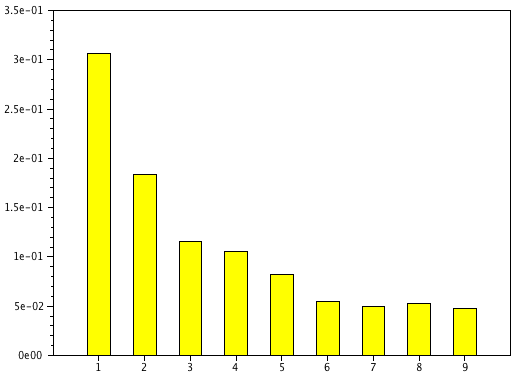 Figure 1
| First digit | Benford’s law | |
|---|---|---|
| 1 | 0.308 | 0.306 |
| 2 | 0.204 | 0.184 |
| 3 | 0.096 | 0.116 |
| 4 | 0.116 | 0.106 |
| 5 | 0.084 | 0.082 |
| 6 | 0.068 | 0.055 |
| 7 | 0.060 | 0.050 |
| 8 | 0.028 | 0.053 |
| 9 | 0.036 | 0.048 |
Peer Reviews
No public reviews on file for this paper yet. If you reviewed it on a platform where reviews are public (OpenReview, ICLR, NeurIPS, ICML), you can paste yours below so the community can read it here.
Videos
No videos yet. Explain this paper in a talk, walkthrough, or lecture? Add one.
On the discrepancy of powers of random variables
Nicolas Chenavier111Université Littoral Côte d’Opale, EA 2797, LMPA, 50 rue Ferdinand Buisson, F-62228 Calais, France. E-mail: [email protected], corresponding author, Dominique Schneider 222Université Littoral Côte d’Opale, EA 2797, LMPA, 50 rue Ferdinand Buisson, F-62228 Calais, France. E-mail: [email protected]
Abstract
Let be a sequence of positive numbers and let be a sequence of positive independent random variables. We provide an upper bound for the deviation between the distribution of the mantissaes of and the Benford’s law. If goes to infinity at a rate at most polynomial, this deviation converges a.s. to 0 as goes to infinity.
Keywords: Benford’s law; discrepancy; mantissa.
AMS 2010 Subject Classifications: 60B10 . 11K38
1 Introduction
A sequence of positive numbers is said to satisfy the first digit phenomenon if
[TABLE]
where is the first digit of , and where denotes the indicator function of any subset . Such a phenomenon was observed by Benford and Newcomb on real life numbers [1, 13]. It is extensively used in various domains, such as fraud detection [14], computer design [8] and image processing [17]. As an extension of the first digit phenomenon, the notion of Benford sequence is introduced as follows. Let be the measure on the interval defined by
[TABLE]
where denotes the logarithm in base of . Let be the mantissa in base of a positive number , i.e. is the unique number in such that there exists an integer satisfying . A set of numbers is referred to as a Benford sequence if for any , we have
[TABLE]
In particular, each Benford sequence satisfies the first digit phenomenon since if and only if , with , . For instance, the sequences , and are Benford. For various examples of sequences of positive numbers whose mantissae are (or approach to be) distributed with respect to , see e.g. [5, 6]. More recently, several authors have provided examples of sequences of random variables whose mantissa distribution converges to [3, 10, 16] or whose the sequence of mantissae is almost surely distributed with respect to . For a wide panorama on Benford sequences, see the reference books [2, 12].
It is well known that a sequence of positive numbers is Benford in base if and only if the sequence of its fractional parts is uniformly distributed in . According to the Weyl’s criterion (see e.g. [9], p7), the sequence is Benford if and only if, for any , we have
[TABLE]
To define a deviation between a sequence and the Benford’s law, the notion of discrepancy is introduced as follows. Let be a sequence of real numbers. The discrepancy modulo 1 of order of , associated with the natural density, is defined as
[TABLE]
For more details on the discrepancy, see e.g. [9], p100–131. For a sequence , if we set , we write . The quantity deals with the deviation between and the distribution of the first terms of since . Hence
[TABLE]
In particular, is Benford if and only if converges to 0 as goes to infinity. Through misuse of language, we also say that is the discrepancy of .
In this paper, we consider the following problem. Let be a sequence of positive independent random variables. We say that is a.s. Benford if the sequence is Benford. As observed in [7], several deterministic sequences at a power tend to be Benford when the power is large enough. The aim of our paper is to provide general conditions on the distribution of the random sequence to ensure that is a.s. Benford for any sequence of positive numbers such that converges to infinity at a rate at most polynomial.
First, we give some notation. In what follows, the function denotes the natural logarithm. For any functions , , we write if and only if . Moreover, we write if and only if there exists a positive number and a real number such that for any .
We are now prepared to state our first theorem, which provides an upper bound for the discrepancy.
Theorem 1**.**
Let be a (deterministic) sequence of positive numbers such that for some . Let be a sequence of positive independent random variables satisfying the following two conditions:
- (i)
there exists such that 2. (ii)
there exists a sequence of nonnegative numbers , with for some , and their exist four constants , such that for large enough and for each , we have
[TABLE]
Then there exist an integrable random variable and a constant such that, for any , we have
[TABLE]
where .
The above theorem is obvious if the upper bound does not converge to 0. However, if , it provides a non-trivial estimate for the discrepancy when goes to infinity at a rate at most polynomial. As a consequence, we obtain the following result.
Corollary 2**.**
Let be such that for some and . Assume that satisfies the assumptions (i) and (ii) for some , with . Then converges a.s. to 0, at a rate of convergence provided in Theorem 1. In particular, the sequence is a.s. Benford.
In particular, if and satisfy the assumptions of Corollary 2, with the more restrictive condition for each , then the discrepancy of can be bounded as follows:
[TABLE]
It is rather surprising that is a.s. Benford for a sequence which converges arbitrarily slowly to infinity. On the opposite, it appears that for several classes of (deterministic) sequences , the sequence is Benford, when converges to infinity at a rate at less polynomial (see e.g. Theorem 2 in [11]). As a second consequence of Theorem 1, the following corollary deals with the case where the sequence is constant.
Corollary 3**.**
Let for each and let be such that the assumptions (i) and (ii) hold for some . Then there exist an integrable random variable and a constant such that, for any , we have
[TABLE]
where .
In particular, as goes to infinity, the sequence tends to be a.s. Benford in the sense that its discrepancy converges to 0 as . In a different context, such a convergence was already observed in Theorem 1 in [7], in which it is stated that two (deterministic) sequences at a large power tend to be Benford.
The assumption (i) of Theorem 1 is few restrictive. Indeed, thanks to the Markov’s inequality, such a condition is satisfied when and are negligible compared to for some . The assumption (ii) of Theorem 1 is in a way classical and is discussed in Remark 1.
Our paper is organized as follows. In Section 2, we prove Theorem 1. This result is illustrated through several examples of standard distributions in Section 3. These examples deal with discrete and continuous random variables respectively. In the rest of the paper, we denote by a generic constant which is independent of , and , but which may depend on other quantities.
2 Proof of Theorem 1
To prove Theorem 1, we apply two well-known inequalities. The first one deals with the discrepancy and is referred to as the Erdös-Turán inequality (see e.g. [RT]).
Theorem 4**.**
(Erdös-Turán inequality) Let be a sequence of real numbers and let . Then, for every integer , we have
[TABLE]
The second inequality which we apply gives a deviation beween a sum of unit random complex numbers and the expectation of this sum. Such a result is due to Cohen and Cuny (Theorem 4.10 in [4]) and is re-written in our context.
Theorem 5**.**
*(Cohen & Cuny, 2006)
Let be a sequence of independent random variables, with values in . Assume that there exists , such that . Let be a sequence of complex numbers. Then there exist universal constants and , such that*
[TABLE]
In the rest of the paper, with a slight abuse of notation, we omit the dependence in , e.g. we write instead of . We are now prepared to prove our first theorem. Proof of Theorem 1. According to the Erdös-Turán inequality, we have for any ,
[TABLE]
Hence,
[TABLE]
First, we provide an upper bound for the term on the bottom. To do it, we take , and . Since , we obtain for large enough that with . Hence, according to the assumption (i), we have . It follows from Theorem 5 that
[TABLE]
In particular, there exists an integrable random variable such that, for any , , we have
[TABLE]
Notice that we have considered a sum over and not over in the above equation because . By taking and , we obtain for any that
[TABLE]
Secondly, we provide an upper bound for the second term in the right-hand side in (2). To do it, let be such that the inequality (1) holds for each . Then
[TABLE]
Bounding by 1 in the first sum and applying the inequality (1) in the second sum for the right-hand side, we get
[TABLE]
Besides, , and . This implies that
[TABLE]
Since and , we have if and otherwise. This together with (2) and (3) implies that
[TABLE]
Optimizing the right-hand side over , we conclude the proof of Theorem 1 by taking
[TABLE]
Remark 1**.**
The assumption given in Equation (1) has been chosen in such a way that it holds when follows the (discrete) uniform distribution on . Indeed, in this case, we have
[TABLE]
According to the Van der Corput’s theorem (see e.g. [9], p17), this shows that
[TABLE]
In particular, this satisfies Equation (1) with , and . However, our assumption (ii) and our assumption on the independence of the random variables remain restrictive. We hope, in a future paper, to extent Theorem 1 with more general conditions.
Remark 2**.**
The main tool to derive the rate of the discrepancy is contained in Theorem 5. Besides, as a consequence of Corollary 3, we deduce that
[TABLE]
In particular, when is large, the sequence tends to be a Benford sequence. However, Theorem 5 is not necessary to derive Equation (4) because the latter can be proved directly by standard arguments. Indeed, it follows from the law of large numbers (for independent non-stationary random variables) and the Erdös-Turán inequality that for all fixed ,
[TABLE]
Besides, according to (1), we know that
[TABLE]
Hence, by taking , this proves that . However, the main contribution of our paper is to provide an explicit rate of convergence for the discrepancy of as goes to infinity.
3 Examples
In this section, we give several examples of sequences of random variables satisfying the assumptions (i) and (ii) of Theorem 1. Our examples deal with discrete and continuous random variables respectively.
3.1 Discrete random variables
The following proposition provides sufficient conditions for discrete random variables to ensure that the assumption (ii) of Theorem 1 is satisfied for .
Proposition 6**.**
Let be a sequence of random variables with finite expectation and such that a.s.. Assume that there exists a sequence of modes such that the sequences and are non-decreasing and non-increasing respectively. Moreover, assume that for some one of the two following cases is satisfied:
- •
Case 1:* and ;*
- •
Case 2:* , and .*
Then for large enough and for each , we have:
[TABLE]
where are two constants.
Proof of Proposition 6. First, we provide a generic upper bound for which is independent of the two above cases. Then we deduce a specific upper bound for this expectation which depends this time on the case which is considered.
To do it, we write . Let be fixed. It follows from the Abel transformation that
[TABLE]
Since converges to 0 as goes to infinity (because ), it is enough prove that
[TABLE]
for some constants . To do it, we apply the following lemma.
Lemma 7**.**
For each , , we have
[TABLE]
Proof of Lemma 7. First, we notice that
[TABLE]
where is the Riemann sum of the function on with regular steps of length . Hence
[TABLE]
where the second inequality comes from the fact that . Besides,
[TABLE]
where the last line is a consequence of the mean value inequality. Integrating the right-hand side over , we get
[TABLE]
This concludes the proof of Lemma 7. According to Lemma 7, we have
[TABLE]
Since the sequences and are non-decreasing and non-increasing respectively, we get
[TABLE]
With standard computations, we get:
[TABLE]
Using the fact that for each , we deduce that
[TABLE]
where
[TABLE]
and
[TABLE]
The inequality (6) is independent of the two cases considered in the assumptions of Proposition 6. Now, we deal with the terms and by discussing these two cases.
- •
Case 1: if for some and , we obtain that . Moreover, since and
[TABLE]
- •
Case 2: if , and for some , we also obtain that and .
This concludes the proof of Proposition 6. We give below three examples of sequences of random variables by checking the assumption (i) of Theorem 1 and one of the two cases of Proposition 6. According to Theorem 1 and Proposition 6, the discrepancy for each example can be bounded as follows:
[TABLE]
In particular, if with and , the sequence is a.s. Benford.
Example 1**.**
Assume that has a geometric distribution with parameter . Here , so that . We also obtain the same order for . In particular, the third conditions of Case 2 are satisfied. Besides, if for some , the assumption (i) holds since
[TABLE]
according to the Markov’s inequality.
Example 2**.**
Let be a random variable with distribution , where is the normalizing constant and . In particular, we have
[TABLE]
since
[TABLE]
Here and the third conditions of Case 2 are satisfied. Indeed, the first one is trivial and for the second one we have . For the third condition, let . According to (7), we have . It follows from the dominated convergence theorem that
[TABLE]
This checks the third condition of Case 2 for each . Besides, the assumption (i) holds since for each and for each , we have
[TABLE]
Example 3**.**
Assume that has a (discrete) uniform distribution in , with , for some , and . Here we take . The two conditions of Case 1 are satisfied. Indeed, the first one holds because . The second one comes from the fact that and Besides, a sufficient and few restrictive assumption on to ensure that the assumption (i) holds is: for some . Notice that if converges to 1, the random variables are asymptotically deterministic. It is not surprising that the property (b) cannot hold in this context since there exist deterministic sequences such that, at any power , the sequences are not Benford.
3.2 Continuous random variables
Let be a sequence of random variables. We first state three properties which imply the assumption (ii) of Theorem 1 when they are simultaneously satisfied.
- (a)
For any , the density of exists and is a piecewise absolutely continuous function. In what follows, we denote by the number of sub-domains of and by the -th sub-domain, with for each . The -th interval is of the form . In particular, is a.e. differentiable on and on the complement. 2. (b)
. 3. (c)
.
Under the above assumptions, the following proposition ensures that the assumption (ii) of Theorem 1 holds, with and for each .
Proposition 8**.**
If the properties hold (a), (b) and (c) hold simultaneously, then for large enough and for each , we have .
Proof of Proposition 8. It is enough to prove the following inequality:
[TABLE]
To do it, we assume without loss of generality that for each , with . In particular, the density is absolutely continuous on and equals 0 on the complement. This gives for any
[TABLE]
In particular, we have provided that the three above properties hold.
Notice that if denotes the density of , we can easily show that satisfies the above assumptions if and only if the ones are satisfied by the density of . This suggests that our assumptions are not very restrictive. We give below three examples of distributions of random variables which satisfy the assumption (i) of Theorem 1 and the three conditions (a), (b) and (c) of Proposition 8. According to Theorem 1 and Proposition 8, the discrepancy for each example can be bounded as follows:
[TABLE]
To obtain the rate of the discrepancy, we have taken and . In particular, if with for some , the sequence is a.s. Benford.
Example 4**.**
If has an exponential distribution with parameter , the properties (a), (b) and (c) hold simultaneously, with . Indeed, the first one is trivially satisfied and for the second and the third ones, we get:
[TABLE]
Besides, for each , we have
[TABLE]
Hence the assumption (i) is satisfied if there exists such that and .
Example 5**.**
Assume that has a standard Fréchet distribution with parameter , i.e. if and otherwise. The property (a) holds. Moreover, if and , we can easily prove that the properties (b) and (c) are satisfied. Besides, the assumption (i) is also satisfied since for each , we have
[TABLE]
where the right-hand side is the term of a convergent series.
Example 6**.**
If has a (continuous) uniform distribution on , with , the properties (a) and (c) hold. Moreover, the property (b) is satisfied when . Besides, a sufficient and few restrictive assumption on to ensure that the assumption (i) holds is: and for some . Unsurprisingly, the assumptions on are very similar to those considered for a (discrete) uniform distribution.
3.3 A numerical illustration
In this section, we give a numerical illustration of a sequence of independent random variables such that is almost a Benford sequence. For each , the distribution of is assumed to be the (continuous) uniform distribution on . This sequence satisfies the assumptions of Theorem 1 (see Example 6). In Table 1, we provide the frequencies of the first significant digit of , with and . It appears that the distribution of frequencies of is close to the Benford’s law.
The reference list from the paper itself. Each links out to its DOI / PubMed record.
- 1[1] F. Benford. The law of anomalous numbers. Proceedings of the American Philosophical Society , (78): 551–572, 1938.
- 2[2] A. Berger, T.P. Hill. An introduction to Benford’s law. Princeton University Press, Princeton, NJ , 2015.
- 3[3] N. Chenavier, B. Massé, and D. Schneider. Products of random variables and the first digit phenomenon, available in https://arxiv.org/abs/1512.06049 , 2015
- 4[4] G. Cohen, C. Cuny. On random almost periodic series and random ergodic theory. Ergodic Theory Dynam. Systems , (26): 683–709, 2006
- 5[5] D. I. A. Cohen, T. M. Katz. Prime numbers and the first digit phenomenon. J. Number Theory , (18): 261–268, 1984
- 6[6] P. Diaconis. The distribution of leading digits and uniform distribution mod mod {\rm mod} 1 1 1 . Ann. Probability , (5): 72–81, 1977
- 7[7] D. Eliahou, B. Massé, D. Schneider. On the mantissa distribution of powers of natural and prime numbers. Acta Math. Hungar. , (139): 49–63, 2013
- 8[8] R. W. Hamming. On the distribution of numbers. Bell System Tech. J. , (49): 1609–1625, 1970