Quantum Coherent Control via Pauli Blocking
Tom Dowdall, Albert Benseny, Thomas Busch, Andreas Ruschhaupt

TL;DR
This paper introduces a novel quantum control method using Pauli blocking to prevent unwanted transitions in fermionic systems, enabling faster adiabatic processes in ultracold atom experiments.
Contribution
The paper presents a new technique leveraging Pauli blocking to accelerate adiabatic quantum control in fermionic systems, demonstrated through ultracold atom applications.
Findings
Pauli blocking effectively prevents unwanted excitations.
The method enables faster adiabatic evolutions.
Insights into the orthogonality catastrophe are gained.
Abstract
Coherent quantum control over many-particle quantum systems requires high fidelity dynamics. One way of achieving this is to use adiabatic schemes where the system follows an instantaneous eigenstate of the Hamiltonian over timescales that do not allow transitions to other states. This, however, makes control dynamics very slow. Here we introduce another concept that takes advantage of preventing unwanted transitions in fermionic systems by using Pauli blocking: excitations from a protected ground state to higher-lying states are avoided by adding a layer of buffer fermions, such that the protected fermions cannot make a transition to higher lying excited states because these are already occupied. This allows to speed-up adiabatic evolutions of the system. We do a thorough investigation of the technique, and demonstrate its power by applying it to high fidelity transport, trap expansion…
Click any figure to enlarge with its caption.
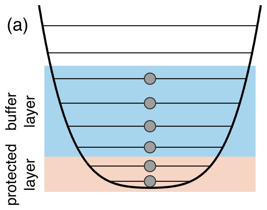 Figure 1
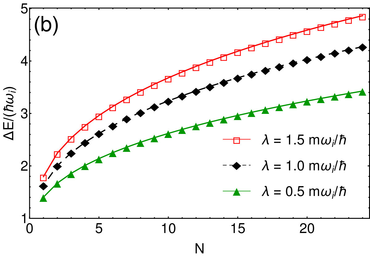 Figure 1
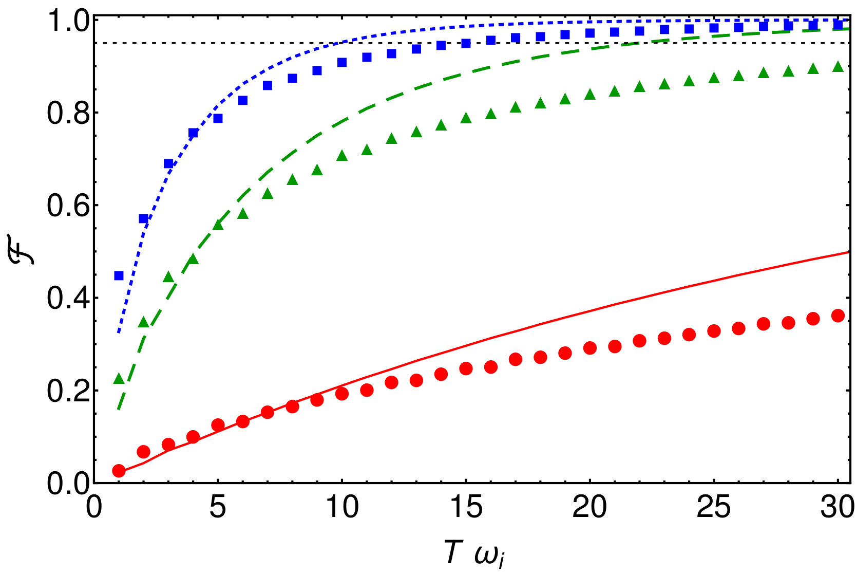 Figure 2
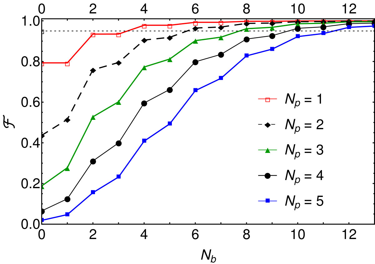 Figure 2
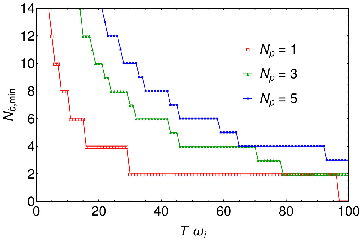 Figure 2
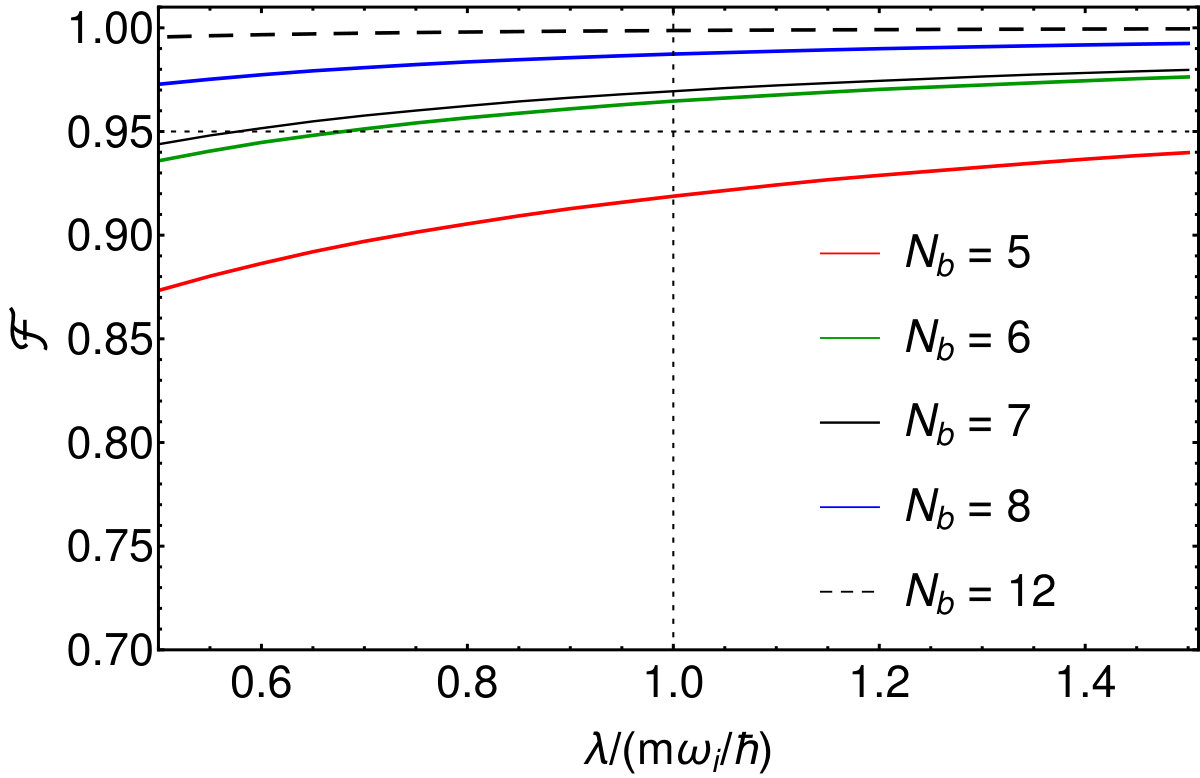 Figure 3
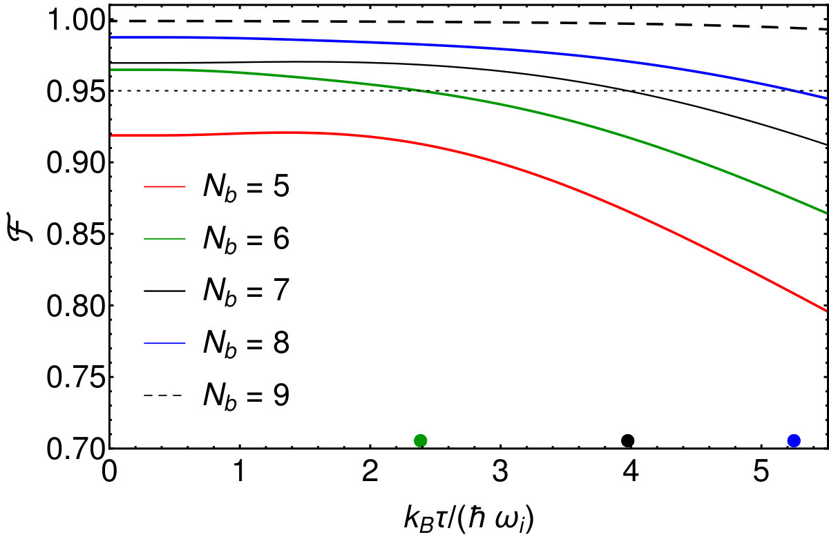 Figure 3
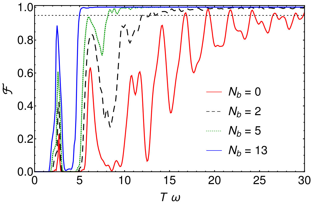 Figure 4
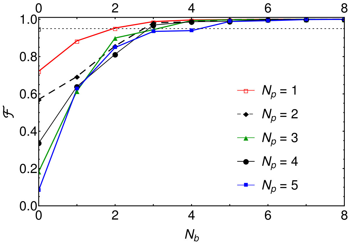 Figure 4
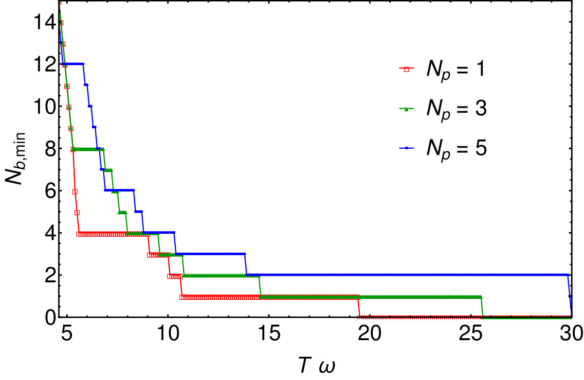 Figure 4
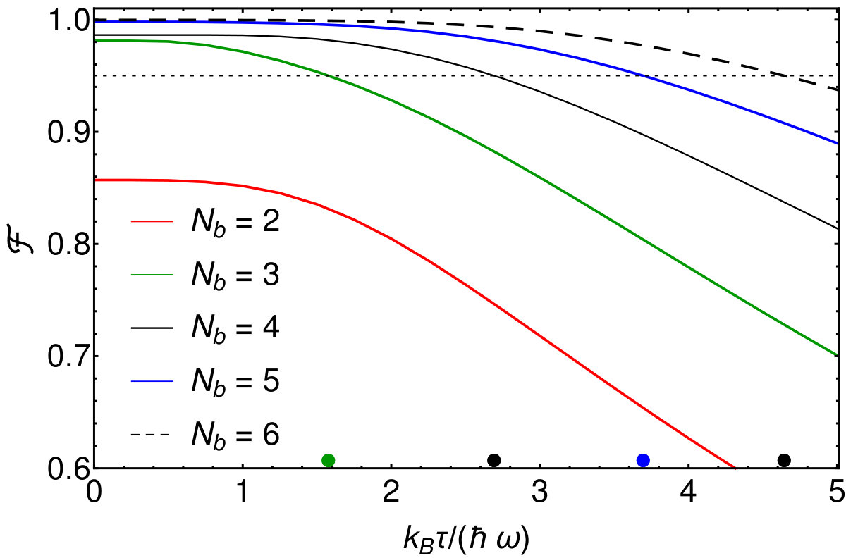 Figure 5
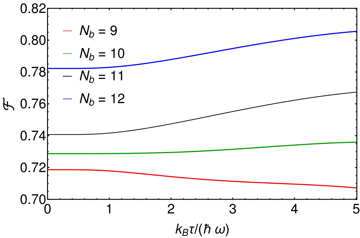 Figure 5
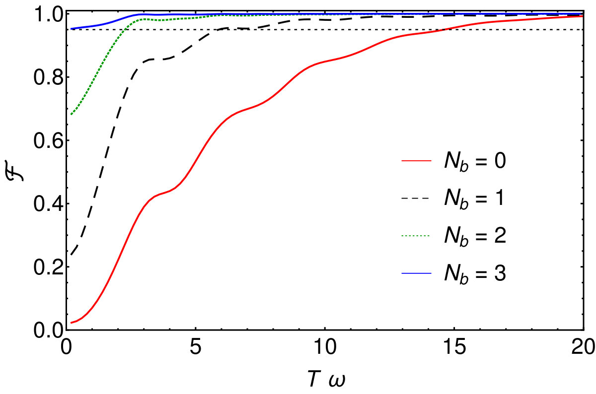 Figure 6
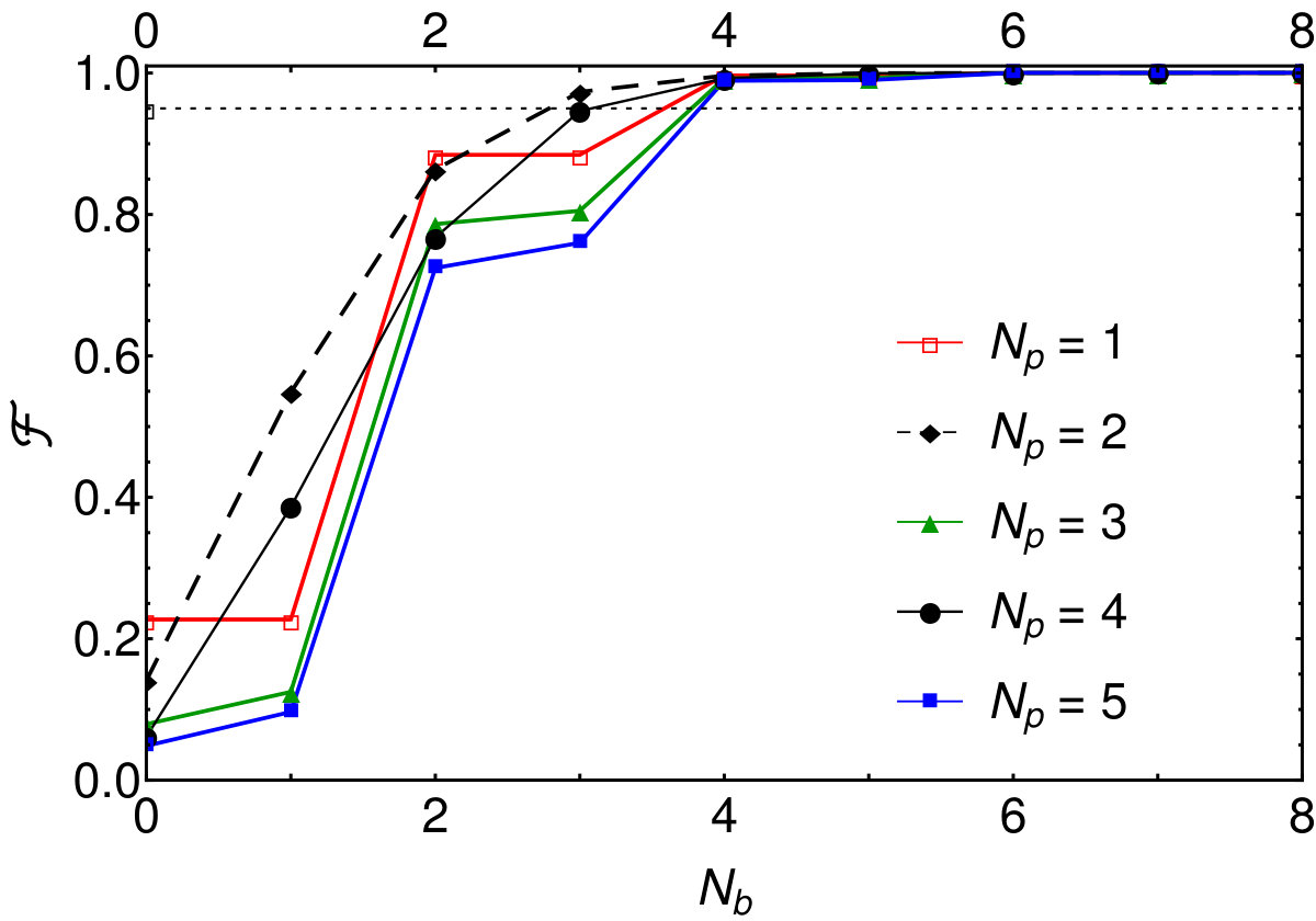 Figure 6
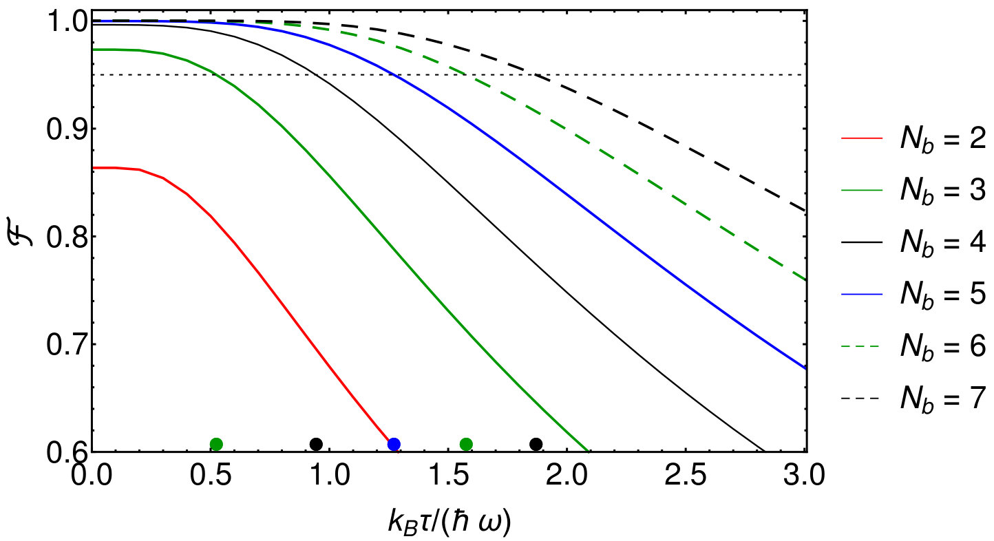 Figure 6
Peer Reviews
No public reviews on file for this paper yet. If you reviewed it on a platform where reviews are public (OpenReview, ICLR, NeurIPS, ICML), you can paste yours below so the community can read it here.
Videos
No videos yet. Explain this paper in a talk, walkthrough, or lecture? Add one.
Quantum Coherent Control via Pauli Blocking
Tom Dowdall
Department of Physics, University College Cork, Cork, Ireland
Albert Benseny
Quantum Systems Unit, Okinawa Institute of Science and Technology Graduate University, 904-0495 Okinawa, Japan
Thomas Busch
Quantum Systems Unit, Okinawa Institute of Science and Technology Graduate University, 904-0495 Okinawa, Japan
Andreas Ruschhaupt
Department of Physics, University College Cork, Cork, Ireland
Abstract
Coherent quantum control over many-particle quantum systems requires high fidelity dynamics. One way of achieving this is to use adiabatic schemes where the system follows an instantaneous eigenstate of the Hamiltonian over timescales that do not allow transitions to other states. This, however, makes control dynamics very slow. Here we introduce another concept that takes advantage of preventing unwanted transitions in fermionic systems by using Pauli blocking: excitations from a protected ground state to higher-lying states are avoided by adding a layer of buffer fermions, such that the protected fermions cannot make a transition to higher lying excited states because these are already occupied. This allows to speed-up adiabatic evolutions of the system. We do a thorough investigation of the technique, and demonstrate its power by applying it to high fidelity transport, trap expansion and splitting in ultracold atoms systems in anharmonic traps. Close analysis of these processes also leads to insights into the structure of the orthogonality catastrophe phenomenon.
pacs:
37.10.Gh Atom traps and guides, 67.85.Lm Degenerate Fermi gases, 05.30.Fk Fermion systems and electron gas
I Introduction
Preparation of and coherent control over many-particle quantum states requires quantum engineering techniques that lead to high fidelities. Adiabatic processes, where the system follows an eigenstate of the time-dependent Hamiltonian, are known to allow for this; however they require that the Hamiltonian is varied sufficiently slowly in order to avoid transitions to other eigenstates messiah_book . This leads to long process times and leaves the system vulnerable to decoherence, reducing also the possible repetition rates of the process.
How quickly or slowly an eigenstate can be followed depends roughly on the distance to the next closest-lying eigenstate messiah_book . Therefore, one strategy for expediting adiabatic processes is to adjust the instantaneous speed of the process with respect to the size of the instantaneous level gap such that the transition probability to unwanted eigenstates remains small during the whole process Guerin_2002 ; Guerin_2011 ; Garaot_2015 . This, however, requires the knowledge of the energy eigenspectrum during the whole process.
In recent years, a number of techniques to speed up adiabatic processes have been developed under the name “shortcuts to adiabaticity” sta_review_1 ; sta_review_2 . One example of these techniques relies on the implementation of an additional counter-diabatic Hamiltonian, which is designed to compensate for any excitations that appear during the finite time evolution process, such that the system does not leave the eigenstates of the original Hamiltonian demirplak_2003 ; berry_2009 ; chen_2010b . However, this additional Hamiltonian can be very complicated and thus be demanding to implement experimentally. Other shortcut techniques are based on Lewis–Riesenfeld invariant inverse engineering chen_2010a , which allow for a fast transfer of all initial eigenstates simultaneously to all final eigenstates (up to a phase).
Generalizing these techniques to many particle systems is not a straightforward task, as the number of degrees of freedom increases exponentially with larger particle numbers. The effects of this are well known and can be seen immediately when considering one of the most simple systems possible, namely an ideal, spin-polarized, one-dimensional Fermi gas at low temperatures: even in the presence of almost perfect single-particle process fidelities, the overlap between two many-particle wavefunctions scales with , where depends on the specific nature of the change between the initial and final Hamiltonian orthocat-1 . This is the so-called orthogonality catastrophe (OC) orthocat-2 ; orthocat-3 , which has recently been examined for systems of ultracold fermions Goold:11 ; Campbell:14
Here, however, we show that this behavior does not necessarily limit the engineering of many-particle states, as the OC does not affect all states inside a Fermi sea in the same way. In fact, one can always find a kernel of particles that is essentially unperturbed, and whose size scales with the overall number of particles. This is due to the fact that transitions inside the Fermi sea are forbidden by the Pauli exclusion principle and lead to the so-called Pauli blocking, which has recently been examined to engineer cold atomic systems Busch:98 ; Ferrari:99 ; Demarco:01 ; OSullivan:09 ; Omran:2015 .
In this work we will consider a system of trapped, ultracold, spin-polarized fermionic atoms, and explore the idea of using Pauli blocking for speeding up adiabatic evolutions. In addition to the ground state layer of particles that should be protected from making transitions we are also adding a buffer layer of particles, see Fig. 1(a). The basic idea now is that only the fermions close to the Fermi edge can make transitions, whereas all atoms inside the Fermi sea need significantly more energy to get excited. Since we are only interested in the protected particles, this will allow to carry out adiabatic processes much faster, as long as the energies introduced by the dynamics do not allow for particles in the protected layer to make transitions. Once the evolution is finished, the buffer fermions can be discarded by, for example, lowering the trap walls Serwane_2011 or inducing spin-flips as in similar techniques for the evaporative cooling of bosons Ketterle_1996 . As this technique can most easily protect ground states, it is particularly well suited to prepare initial states in potentials where direct ground-state cooling is challenging.
The idea we present relies on the specific form of the energy spectrum around the Fermi edge. If the Fermi edge is close to the continuum states in a finite height potential, it is not guaranteed that the process we investigate will work. However, if the spectrum becomes increasingly sparse beyond the Fermi edge (for example in anharmonic trapping potentials, see Fig. 1(b)), significant speedups can be obtained. In fact, in this limit the idea of Hilbert space engineering through quantum statistics is largely independent of the potential shape, i.e. the exact form of the Hamiltonian.
Since the technique we discuss below will protect the lower motional energy states, and since the protection is done by the presence of a Fermi sea, it requires fermionic samples that are deep within the quantum degenerate regime. For neutral atoms these can be produced routinely in laboratories worldwide these days DeMarco:99 ; Partridge:06 ; Shin:08 and since the removal of the higher energy particles from a trap can also be done using standard techniques, we will concentrate in this paper on the control process itself.
In the following we will first introduce the system we investigate and define and discuss the process fidelity as our figure of merit. We will then apply the method in detail to three specific control tasks in Sec. III, and conclude in Sec. IV.
II System and fidelity
II.1 Fermion state
We consider a gas of spin-polarized fermions that formally consists of particles whose state we want to protect and particles that form a buffer layer (see Fig. 1(a)), so that the overall number of particles is . Since at ultracold temperatures the dominant scattering interaction is of symmetric s-wave form, such gases can be efficiently described as non-interacting and they therefore form a perfect Fermi sea at zero temperature Giorgini:08 . This also means that the time evolution of the many-particle wave function, , can be obtained by solving the single-particle Schrödinger equations for each state within the Fermi sea
[TABLE]
where the shape and time-dependence of the potential, , depends on the particular task that is to be implemented. The many particle wavefunction then follows from calculating the Slater determinant as
[TABLE]
where consists of all the permutations of the set .
II.2 Process fidelity
In the following we will consider processes where the lowest eigenstates of an initial Hamiltonian are occupied by relevant particles and we aim at having this subset of the Fermi sea to be undisturbed during the evolution towards the final Hamiltonian. In order to quantify how well the process works we calculate the overlap between the evolved state at the final time , , and the lowest lying eigenstates of the Hamiltonian at the end of the process. In detail, we define the fidelity of the process as
[TABLE]
where is an element of the fermionic subspace of the -particle Hilbert space and the measurement operator is defined as
[TABLE]
The operator checks the occupation probability of the -th eigenstate of the Hamiltonian, provided that , and, as we are not interested in the population of levels above , acts as the identity for .
Let be the projector on the fermionic subspace . For , we have where . One can show by using the fermionic number basis states that
[TABLE]
where the sum is over all vectors fulfilling for and . From its structure it is clear that the operator is a projector. This proves that always as it should be for a meaningful fidelity definition.
The fidelity (3) can then be rewritten as (see Appendix for details)
[TABLE]
where the first sum is over all mappings with for (which can be also viewed as all subsets of cardinality of the set ). As mentioned above, the states can be obtained from the single-particle Schrödinger equation (1).
From Eq. (7), it also follows that , i.e. that increases monotonically with the number of buffer particles . This can be seen because
[TABLE]
where are all a subset of cardinality of the set and are all a subset of cardinality of the set . Note that from this property and the fact that is bounded by , we know that the limit must exist, but it is not necessarily 1.
II.3 Adiabaticity and shortcuts
Let us first look at schemes which work perfectly in the adiabatic limit, i.e., for . In this limit one gets where the are phases. It immediately follows from Eq. (7) that . To be more general, if is large but finite, we get that where the phase of can be chosen in such a way that . Based on this, we can make a series expansion of the fidelity in the small parameter as
[TABLE]
where is an expression independent of . However, it can be seen that all terms which depend on are always positive and therefore improve the fidelity. This coincides with the general monotonicity of the fidelity in shown above.
Another special case are settings where shortcuts to adiabaticity techniques can be applied exactly, like for example the expansion of a harmonic trap chen_2010a or the transport in a harmonic trap torrontegui_2011 . One can see from the above equation that one would obtain exactly for arbitrary numbers of particles on arbitrary timescales. In the following, we will therefore concentrate on settings where a shortcut to adiabaticity cannot be found easily, in particular anharmonic settings.
II.4 Temperature effects
To extend this approach to the case of a finite temperature , the initial state is of canonical form and the probability for a specific occupation at initial time is given by
[TABLE]
Here is the partition function and is the Boltzmann constant. The sum is over all functions with , i.e. are the numbers of the energy eigenstates occupied by the fermions and the are the ordered eigenenergies of the Hamiltonian at the initial time. The finite-temperature fidelity will then be the average over the fidelities of the different possible permutations of the particles
[TABLE]
where is the fidelity defined similar to the one above with just the states in initially occupied instead of :
[TABLE]
Note that while this sum is in principle infinite, we will truncate it for its numerical evaluation at a maximal energy level chosen such that the result is practically independent from the exact level of truncation.
III Control tasks
In this section we focus on particles trapped in potentials with significant anharmonicities, such that these cannot be treated as perturbations, and discuss three manipulation examples: expansion, transport, and splitting of the trap. For small (or zero) trap anharmonicity shortcuts for expansion and transport have been derived sta_review_1 ; torrontegui_2011 ; torrontegui_2012a ; torrontegui_2012b ; STA_anharm_trans and shortcuts related to the splitting can be found, for example, in torrontegui_2013 ; martinez_2013 .
This broad variety of tasks will show that, in contrast to other shortcut-to-adiabaticity protocols, the idea presented here is insensitive to the details of how the trap parameters are varied in time and does not require any specific time-dependence parameter functions which might be very complex and hard to implement experimentally. The only parameter is the number of buffer particles, , and we will show below how the fidelity depends on the size of the buffer for each of the three processes.
III.1 Trap expansion
We first consider the expansion of the trapping potential, which we choose to be of the form
[TABLE]
and in which the anharmonicity is quantified by the parameter . We set such that the anharmonicity is significant and far from being just a small perturbation.
For the control task the trapping frequency is changed from at to at and we consider two different forms of the time-dependence, linear and sinusoidal, respectively given by
[TABLE]
The resulting fidelities for both schemes are shown in Fig. 2(a) for . One can clearly see that adding just a small number of buffer particles leads to significantly larger , even at total times for which the fidelity without buffer particles was very low. We also see that this is independent of the control scheme, underlining the fact that our method does not depend on the precise time-dependence of the control parameters. Nonetheless, it can be seen that the sinusoidal scheme generally results in larger than the linear scheme for fixed and . Since both schemes yield roughly similar results we will in the following focus on the sinusoidal scheme only.
The dependence of the fidelity on the number of buffer particles for different numbers of protected particles is shown in Fig. 2(b) for a fixed process time of . The fidelity increases monotonically with increasing (for fixed ), agreeing with the general property of the fidelity derived in Sec. II.
In addition, it is interesting to note that adding an even number of particles is more effective than adding an odd number. This can be understood by first considering the extreme case of (red line in Fig. 2(b)), where it can be seen that, if one add a single buffer particle to an even number of buffer particles, the process fidelity does not change. The reason for this is that expansion is a symmetric operation with respect to the center of the trap, i.e. the Hamiltonian commutes with the parity operator. Therefore states of different parity do not couple and for the subspace of buffer particles in odd eigenstates completely decouples from the subspace of the single, protected particle (as the ground state is even) and also from the buffer particles in even eigenstates. The fidelity then depends only on the even subspace and adding an additional odd buffer particle has no effect. For larger , both subspaces are involved in the fidelity, making the situation more complex and the effect less prominent.
Fig. 2(b) also illustrates the effect of the OC, as one can see that fidelities decrease dramatically with larger system sizes (larger ). However, it is also worth pointing out that in our situation this is slightly surprising, as due to the trap anharmonicity, the Fermi gap is bigger for larger , see Fig. 1(b), and one could therefore expect the OC to be suppressed for larger systems at fixed . Nevertheless, Fig. 2(b) clearly shows that adding more particles to the system increases the fidelity of the relevant, lower lying many-body state, and therefore allows to beat the OC.
In all cases a fidelities can be achieved by adding a large enough number of buffer particles and Fig. 2(c) shows the relation between the process time and the minimal number of buffer particles needed for achieving for all process times larger than . It can clearly be seen that smaller must be combined with a larger number of buffer particles, , to result in the desired threshold fidelity.
Next, we study the effects of the potential shape and the temperature on our scheme and start by considering the dependence on for different (relevant, non-perturbative) anharmonicities . The results shown in Fig. 3(a) confirm that this method does not require a detailed knowledge of the trapping potential, as for the fidelity stays always above the threshold fidelity of for the whole range of values shown. In fact, we note that the fidelity increases with as our scheme takes advantage of the increased energy gap at the Fermi energy for larger (see again Fig. 1(b)).
Finite temperature results are shown in Fig. 3(b) for different numbers of buffer particles (with fixed ). and it can be seen that the scheme is quite stable under temperature perturbations. Increasing temperatures can be compensated by increasing the number of buffer particles to achieve the same target fidelity: should be increased by one to compensate for an increase in temperature of the order of (see the dots in Fig. 3(b)). This is also what one would expect heuristically as the “width” of the edge in the Fermi–Dirac distribution is of the order of and the energy gap is of the order . As one might expect, the increase of the fidelity is again monotonic with increasing with finite temperature for the shown parameter range.
III.2 Transport
The second dynamical scheme we examine is the spatial translation of the trapping potential described by
[TABLE]
and we choose the movement of the trap center between and to be of the form
[TABLE]
Let , and we set . The resulting fidelities are shown in Fig. 4(a) for and one can see that, similarly to the expansion scheme, fidelities of can be achieved by increasing the number of buffer particles instead of increasing the total time . In this case, however, the fidelities exhibit oscillations for shorter , giving high fidelities for some specific final times (similar to couvert_2008 ).
In Fig. 4(b) we examine how the fidelity depends on the number of buffer particles for different numbers of protected particles (for a fixed process time ). As expected, adding buffer particles always increases the fidelity (see again also Sec. II). However, it is worth pointing out certain differences compared to the expansion scheme (see Fig. 2(a)). First, adding a single buffer particle always has a significant effect and second, the fidelity is now not monotonic in (for fixed and , compare to Fig. 2(b)): all fidelity lines for the different cross the threshold line of given enough .
Figure 4(c) shows the relation between the process time and the minimal number of buffer particles required to reach for all process times larger than or equal to . Similar to the expansion scheme, goes to 0 for large enough and the required buffer is increasing for shorter process times . In addition, does not have a strong dependence on in the transport case.
The relation between and temperature , for different values of (with fixed , ), is shown in Fig. 5(a). One can see that the scheme is again stable against temperature perturbation, however, for increasing temperature the number of buffer particles has to be increased to still achieve a fidelity . Again, from the dots on the horizontal axis it can be seen that has to be increased by one if the temperature increases by an order of . Again, we note that for the temperatures shown there is still the monotonic increase of the fidelity with increasing .
It is also interesting to note that the fidelity in general does not always decrease monotonically with increasing temperature. This can be seen in Fig. 5(b), where a linear transport scheme is considered and an increase in fidelity is visible in certain temperature ranges. The reason for this lies in the internal structure of the Fermi sea at finite temperatures, which allows for highly complex dynamics.
III.3 Splitting
In our final example we will discuss the process where raising a Gaussian barrier at the center of a harmonic trap leads to a splitting of the atomic cloud. For this we chose
[TABLE]
where again . The time dependence of the barrier height chosen as
[TABLE]
where is the initial height of the barrier at before the splitting and after the process. Similarly to the case of expansion, splitting is a symmetric operation , i.e. the Hamiltonian is commuting with the parity operator. As such it is expected that even numbers of additional particles are more effective than are odd numbers. Splitting is also quite distinct from the other manipulations in that it affects higher energy states in the trap less, whereas transport or expansion affect the whole spectrum of states in the trap. In the following, we set and , which lead to a final separation in two wells for approximately the 18 lowest energy eigenstates.
In Fig. 6(a) one can see that, as expected, increasing gives higher fidelities on shorter timescales and increases monotonically with . In fact, the process is very robust and already for a fidelity of can be achieved for almost instant timescales.
The dependence of the fidelity on is shown for different in Fig. 6(b). For odd numbers of particle one can see an effect similar to the one observed in the expansion process, where an even number of buffer particles is needed to see an increase in fidelity. This can again be understood by considering the symmetric nature of the splitting dynamics. However, while one would naively expect the same for states with even numbers of particles , it is absent in this case. The reason for this can be found in the specific structure of the eigenspectrum of the split trap, where for our parameters successive even and odd eigenstates are effectively energetically degenerate. An even number of particles in the system therefore has two particles with energies close to the Fermi edge and adding any number of buffer particles will lead to an increase in fidelity as one possible transition is blocked.
Finally, from Fig. 6(c), one can see that the splitting is slightly more sensitive to temperature than the previous two operations. The dots on the horizontal axis show heuristically that an additional buffer particle is required for every increase in temperature of about , while in the previous two schemes this was about .
IV Conclusion
In this work we have explored the idea of using Pauli blocking for speeding up adiabatic evolution by using an additional layer of buffer particles to protect the lowest-energy fermions when the system parameters are dynamically changed. We have presented a thorough investigation, both analytical and numerical, showing that the presence of this additional layer allows the speed-up of adiabatic manipulations without exciting unwanted transitions. By discussing three different examples, we have demonstrated that this method is robust and applicable to a wide range of scenarios.
The proposed technique is particularly well suited to protect ground states during changes of the external potential, resulting in a speed-up of ground state preparation in potentials for which these states cannot easily be prepared directly with high fidelity. The method does not require precise knowledge of the shape of the trap or the energy spectrum of the system. It is also insensitive to the details of how the trap parameters are varied in time and no specific time-dependence of the parameter functions is necessary, which might be very complex and hard to implement experimentally. All this makes it a very robust and readily applicable technique.
Finally, the presented study gives a deeper insight into the phenomenon of the orthogonality catastrophe. We have shown that the fidelity of a subsystem can be much larger than the one of the full many-body system and in particular, that the particles close to the Fermi edge play a much stronger role in the effect of the many-body state becoming orthogonal.
Acknowledgments
We are grateful to David Rea for useful discussion and commenting on the manuscript. TD acknowledges support by the Irish Research Council (GOIPG/2015/3195). This work was supported by the Okinawa Institute of Science and Technology Graduate University.
Appendix A Calculation of the fidelity
We calculate the fidelity of the final state, , with the measurement operator defined by Eq. (4), where is the state of our -fermion wave function after some unitary time evolution. We want to calculate as a function of the single-particle states , cf. Eq. (2). Expanding the definitions of and , we get
[TABLE]
Since the are orthogonal before manipulation (as eigenstates of the Hamiltonian), they remain orthogonal after the unitary evolution. Let us also define and , so that
[TABLE]
We see that only the permutations that fulfill for contribute to the sum. This allows us to rewrite the contributing permutations as and . should be a permutation with for and for . and are then permutations on such that they permute but act as the identity on . Note that there is a one-to-one correspondence between and the pair . Then we get
[TABLE]
This fidelity is independent of . Therefore, for each we can define a mapping by for such that for . Note that each can also be viewed as a subsets of cardinality of the set . As different result in the same , this allows us to write the fidelity as
[TABLE]
which corresponds to Eq. (7).
The reference list from the paper itself. Each links out to its DOI / PubMed record.
- 1(1) A. Messiah, Quantum mechanics , Elsevier Science B.V. (1961).
- 2(2) S. Guérin, S. Thomas, and H. R. Jauslin, Phys. Rev. A 65 , 023409 (2002).
- 3(3) S. Guérin, V. Hakobyan, and H. R. Jauslin, Phys. Rev. A 84 , 013423 (2011).
- 4(4) S. Martínez-Garaot, A. Ruschhaupt, J. Gillet, Th. Busch, and J. G. Muga, Phys. Rev. A 92 , 043406 (2015).
- 5(5) E. Torrontegui, S. Ibáñez, S. Martínez-Garaot, M. Modugno, A. del Campo, D. Guéry-Odelin, A. Ruschhaupt, X. Chen, and J. G. Muga, Adv. At. Mol. Opt. Phys. 62 , 117 (2013).
- 6(6) A. Ruschhaupt and J. G. Muga, J. Mod. Optics 61 , 828 (2013).
- 7(7) M. Demirplak and S. A. Rice, J. Phys. Chem. A 107 , 9937 (2003).
- 8(8) M. V. Berry, J. Phys. A 42 , 365303 (2009).