This paper introduces a finitary analogue of the downward Löwenheim-Skolem property for finite structures, called $ ext{ extdollar} ext{ extdollar} ext{ extdollar} ext{ extdollar}$-EBSP, demonstrating its presence in various classes and its algorithmic implications.
Contribution
The paper defines the $ ext{ extdollar} ext{ extdollar} ext{ extdollar} ext{ extdollar}$-EBSP property, proves its prevalence in multiple classes, and shows how it enables linear-time algorithms for property checking.
Findings
01
$ ext{ extdollar} ext{ extdollar} ext{ extdollar} ext{ extdollar}$-EBSP holds for classes like posets, trees, and graphs.
02
The property is preserved under certain class operations.
03
Linear fixed-parameter tractable algorithms are developed for property verification.
Abstract
We present a model-theoretic property of finite structures, that can be seen to be a finitary analogue of the well-studied downward L\"owenheim-Skolem property from classical model theory. We call this property as the *L-equivalent bounded substructure property*, denoted L-EBSP, where L is either FO or MSO. Intuitively L-EBSP states that a large finite structure contains a small "logically similar" substructure, where logical similarity means indistinguishability with respect to sentences of L having a given quantifier nesting depth. It turns out that this simply stated property is enjoyed by a variety of classes of interest in computer science: examples include various classes of posets, such as regular languages of words, trees (unordered, ordered or ranked) and nested words, and various classes of…
\begin{array}[]{lllll}&(\Xi(\mathfrak{B}),\bar{d}_{1},\ldots,\bar{d}_{n})&\models&R(x_{1},\ldots,x_{n})&\\
\mbox{iff}&(\mathfrak{B},\bar{d}_{1},\ldots,\bar{d}_{n})&\models&\Xi(R)(\bar{x}_{1},\ldots,\bar{x}_{n})&\mbox{(by
Proposition~{}\ref{prop:relating-transductions-applications-to-structures-and-formulae})}\\
\mbox{iff}&(\mathfrak{B},\bar{d}_{1},\ldots,\bar{d}_{n})&\models&\bigwedge_{i=1}^{i=n}\xi(\bar{x}_{i})~{}\wedge~{}\xi_{R}(\bar{x}_{1},\ldots,\bar{x}_{n})&\mbox{(by defn. of $\Xi(R)$; see~{}\cite[cite]{[\@@bibref{}{makowsky}{}{}]})}\\
\end{array}
\begin{array}[]{lllll}&(\mathfrak{B},\bar{d}_{1},\ldots,\bar{d}_{n})&\models&\bigwedge_{i=1}^{i=n}\xi(\bar{x}_{i})~{}\wedge~{}\xi_{R}(\bar{x}_{1},\ldots,\bar{x}_{n})&\\
\mbox{iff}&(\mathfrak{A},\bar{d}_{1},\ldots,\bar{d}_{n})&\models&\bigwedge_{i=1}^{i=n}\xi(\bar{x}_{i})~{}\wedge~{}\xi_{R}(\bar{x}_{1},\ldots,\bar{x}_{n})&\\
\mbox{iff}&(\mathfrak{A},\bar{d}_{1},\ldots,\bar{d}_{n})&\models&\Xi(R)(\bar{x}_{1},\ldots,\bar{x}_{n})&\mbox{(by definition of
$\Xi(R)$)}\\
\mbox{iff}&(\Xi(\mathfrak{A}),\bar{d}_{1},\ldots,\bar{d}_{n})&\models&R(x_{1},\ldots,x_{n})&\mbox{(by
Proposition~{}\ref{prop:relating-transductions-applications-to-structures-and-formulae})}\\
\end{array}
Peer Reviews
No public reviews on file for this paper yet. If you reviewed it on a platform where reviews are public (OpenReview, ICLR, NeurIPS, ICML), you can paste yours below so the community can read it here.
Videos
No videos yet. Explain this paper in a talk, walkthrough, or lecture? Add one.
Full text
A Finitary Analogue of the Downward Löwenheim-Skolem Property
Abhisekh Sankaran
Department of Computer Science and Engineering,
Indian
Institute of Technology (IIT) Bombay, India
We present a model-theoretic property of finite structures, that can
be seen to be a finitary analogue of the well-studied downward
Löwenheim-Skolem property from classical model theory. We call this
property as the L-equivalent bounded substructure
property, denoted L-EBSP, where L is either FO or
MSO. Intuitively L-EBSP states that a large finite structure
contains a small “logically similar” substructure, where logical
similarity means indistinguishability with respect to sentences of
L having a given quantifier nesting depth. It turns out that
this simply stated property is enjoyed by a variety of classes of
interest in computer science: examples include various classes of
posets, such as regular languages of words, trees (unordered, ordered
or ranked) and nested words, and various classes of graphs, such as
cographs, graph classes of bounded tree-depth, those of bounded
shrub-depth and n-partite cographs. Further, L-EBSP remains
preserved in the classes generated from the above by operations that
are implementable using quantifier-free translation schemes. We show
that for natural tree representations for structures that all the
aforementioned classes admit, the small and logically similar
substructure of a large structure can be computed in time linear in
the size of the representation, giving linear time fixed parameter
tractable (f.p.t.) algorithms for checking L definable
properties of the large structure. We conclude by presenting a
strengthening of L-EBSP, that asserts “logical self-similarity
at all scales” for a suitable notion of scale. We call this the
logical fractal property and show that most of the classes
mentioned above are indeed, logical fractals.
1 Introduction
The downward Löwenheim-Skolem theorem is one of the earliest results
of classical model theory. This theorem, first proved by Löwenheim
in 1915 [21], states that if a first order (henceforth,
FO) theory over a countable vocabulary has an infinite model, then it
has a countable model. In the mid-1920s, Skolem came up with a more
general statement: any structure A over a countable vocabulary
has a countable “FO-similar” substructure. Here, “FO-similarity”
of two given structures means that the structures agree on all
properties than can be expressed in FO. This result of Skolem was
further generalized by Mal’tsev in 1936 [23], to what is
considered as the modern statement of the downward Löwenheim-Skolem theorem: for any
infinite cardinal κ, any structure A over a countable
vocabulary has an elementary substructure (an FO-similar substructure
having additional properties) that has size at most κ. The
downward Löwenheim-Skolem theorem is one of the most important results of classical model
theory, and indeed as Lindström showed in 1969 [20],
FO is the only logic (having certain well-defined and reasonable
closure properties) that satisfies this theorem, along with the
(countable) compactness theorem.
The downward Löwenheim-Skolem theorem is a statement intrinsically of infinite
structures, and hence does not make sense in the finite when taken as
is. While preservation and interpolation theorems from classical model
theory have been actively studied over finite
structures [1, 2, 26, 14, 17, 25, 27, 3, 32, 6, 28, 5, 18], there is very little study of
the downward Löwenheim-Skolem theorem (or adaptations of it) in the finite
([15, 33] seem to be the only studies of this
theorem in the contexts of finite and pseudo-finite structures
respectively). In this paper, we take a step towards addressing this
issue. Specifically, we formulate a finitary analogue of the
model-theoretic property contained in the downward Löwenheim-Skolem theorem, and show that
classes of finite structures satisfying this analogue indeed abound in
computer science. We call this analogue the L-equivalent
bounded substructure property, denoted L-EBSP(S), where
L is one of the logics FO or MSO, and S is a class
of finite structures (Definition 3.1). Intuitively,
this property states that over S, for each m, every structure
A contains a small substructure B that is
“L[m]-similar” to A, where
L[m] is the class of all sentences of L that
have quantifier nesting depth at most m. In other words, B
and A agree on all properties that can be described in
L[m]. The bound on the size of B is given by a
“witness” function that depends only on m (when L and
S are fixed). It is easily seen that L-EBSP(S) has
strong resemblance to the model-theoretic property contained in the
downward Löwenheim-Skolem theorem, and can very well be seen as a finitary analogue of a
version of the downward Löwenheim-Skolem theorem that is “intermediate” between the
versions of this theorem by Skolem and Mal’tsev.
The motivation to define L-EBSP(S) came from our investigations
over finite structures, of a generalization of the classical Łoś-Tarski
preservation theorem from model theory, that was proved
in [31]. This generalization, called the
generalized Łoś-Tarski theorem at level k, denoted GLT(k),
gives a semantic characterization, over arbitrary structures, of
sentences in prenex normal form, whose quantifier prefixes are of the
form ∃k∀∗, i.e. a sequence of k existential
quantifiers followed by zero or more universal quantifiers. The Łoś-Tarski
theorem is a special case of GLT(k) when k equals
0. Unfortunately, GLT(k) fails over all finite structures for all
k≥0 (like most preservation theorems do [26]), and worse
still, also fails for all k≥2, over the special classes of
finite structures that are acyclic, of bounded degree, or of bounded
tree-width, which were identified by Atserias, Dawar and
Grohe [5] to satisfy the Łoś-Tarski theorem. This
motivated the search for new (and possibly abstract) structural
properties of classes of finite structures, that admit GLT(k) for
each k. It is in this context that a version of L-EBSP(S) was
first studied in [30]. The present paper takes that
study much ahead. (Most of the results of this paper are contained in
the author’s Ph.D. thesis [29].)
The contributions of this paper are as described below.
1. A variety of classes of interest in computer science satisfy
L-EBSP: Our property presents a unified framework, via logic,
for studying a variety of classes of finite structures that are of
interest in computer science. The classes that we consider are broadly
of two kinds: special kinds of labeled posets and special kinds of
graphs. For the case of labeled posets, we show L-EBSP holds for
words, trees (of various kinds such as unordered, ordered, ranked, or
“partially” ranked), and nested words over a finite alphabet, and
all regular subclasses of these
(Theorem 5.1). For
each of these classes, we also show that L-EBSP holds with
computable witness functions. While words and trees have had a long
history of studies in the literature, nested words are much
recent [4], and have attracted a lot of attention as
they admit a seamless generalization of the theory of regular
languages and are also closely connected with visibly pushdown
languages. For the case of graphs, we show L-EBSP holds for a
very general, and again very recently defined, class of graphs called
n-partite cographs, and all hereditary subclasses of this
class (Theorem 5.5). This
class of graphs, introduced in [13], jointly generalizes
the classes of cographs (which includes several interesting graph
classes such as complete r-partite graphs, Turan graphs, cluster
graphs, threshold graphs, etc.), graph classes of bounded tree-depth
and those of bounded shrub-depth. Cographs have been well studied
since the ’80s [9] and have been shown to admit
fast algorithms for many decision and optimization problems that are
hard in general. Graph classes of bounded tree-depth and bounded
shrub-depth are much more recently defined [24, 13] and have become particularly prominent in the context
of investigating fixed parameter tractable (f.p.t.) algorithms for
MSO model checking, that have elementary dependence on the
size of the MSO sentence (which is the
parameter) [12, 13]. This line of
work seeks to identify classes of structures for which Courcelle-style
algorithmic meta-theorems [16] hold,
but with better dependence on the parameter than in the case of
Courcelle’s theorem (which is unavoidably
non-elementary [11]). A different and important line of
work shows that FO and MSO are equal in their expressive powers
over graph classes of bounded tree-depth/shrub-depth
[12, 10]. Since each
of the graph classes mentioned above is a hereditary subclass of the
class of n-partite cographs for some n, each of these satisfies
L-EBSP, further with computable witness functions, and further
still, even elementary witness functions in many cases.
We give methods to construct new classes of structures satisfying
L-EBSP from classes known to satisfy L-EBSP. Specifically,
we show that L-EBSP remains preserved under a wide range of
operations on structures, that have been well-studied in the
literature: unary operations like complementation, transpose and the
line graph operation, binary “sum-like” operations [22]
such as disjoint union and join, and binary “product-like”
operations that include various kinds of products like the Cartesian,
tensor, lexicographic and strong products. All of these are examples
of operations that can be implemented using, what are called,
quantifier-free translation
schemes [22, 16]. We show that
FO-EBSP is always closed under such operations, and MSO-EBSP is
closed under such operations, provided that they are unary or sum-like
(Theorem 5.7). In both
cases, the computability/elementariness of witness functions is
preserved under the operations.
2. Linear time f.p.t. algorithms for deciding
L properties of structures: For each of the classes
mentioned above (including those generated using the various
operations) and for natural representations of structures in these
classes, we give linear time f.p.t. algorithms for deciding properties
of structures, that can be defined in L. The structures in the
above classes have natural tree representations in which the
leaf nodes of the tree represent simple substructures and the internal
nodes represent operations that produce new structures upon being fed
with input structures. Given such a tree representation for a
structure, we perform appropriate “prunings” of, and “graftings”
within, the tree, such that the resultant tree represents an
L[m]-similar proper substructure of the original
structure. Two key technical elements that are employed to perform
these prunings and graftings are the finiteness of the index of the
L[m]-similarity relation (which is an equivalence
relation) and a Feferman-Vaught kind composition property of
the operations used in the tree representations. The latter means that
the “L[m]-similarity class” of the structure
produced by an operation is determined by the multi-set of the
L[m]-similarity classes of the structures that are
input to the operation, and further (in the case of operations having
arbitrary finite arity), determined only by a threshold number of
appearances of each L[m]-similarity class in the
multi-set, with the threshold depending solely on m. These
technical features enable generating the “composition
functions” uniformly for any operation for any given m, and the
composition functions thus generated, in turn, enable doing the
compositions in time linear in the arity of the operation. Using
these, we get linear time f.p.t. algorithms that when given an
L sentence of quantifier nesting depth m (the parameter) and
a tree t as inputs, perform the aforementioned prunings and
graftings in t iteratively to produce a small subtree that
represents a small L[m]-similar substructure (the
“kernel”, in the f.p.t. parlance) of the structure represented by
t. The techniques mentioned above have been incorporated int
a single abstract result concerning tree representations
(Theorem 4.2). Given
that this result gives unified explanations for the good computational
properties of many interesting classes, we believe it might be of
independent interest.
3. A strengthening of L-EBSP and connections with
fractals: Fractals are classes of mathematical structures that
exhibit self-similarity at all scales. That is, every structure in the
class contains a similar (in some technical sense) substructure at
every scale of sizes less than the size of the structure. Well-known
examples of fractals in mathematics include the Mandelbrot set, the
Menger Sponge and the Koch snowflake. Remarkably, fractals are not
limited to only mathematics, but in fact abound nearly everywhere in
nature. Tree branching, cloud structures, galaxy clustering, fern
shapes, and crystal growth patterns are some of a wide range of
natural phenomena that exhibit
self-similarity [7].
In the light of fractals, we observe that the L-EBSP property
indeed asserts “logical self-similarity” at “small scales”. We
formulate a strengthening of the L-EBSP property, that asserts
logical self-similarity at all scales, for a suitable notion of scale
(Definition 6.1). We call this the
logical fractal property, and call a class satisfying this
property as a logical fractal. Remarkably, it turns out that
the aforementioned posets and graph classes, including those
constructed using many of the aforementioned operations, are all
logical fractals (Proposition 6.3). The
classical downward Löwenheim-Skolem theorem indeed shows that the class of all infinite
structures satisfies an “infinitary” variant of the logical fractal
property. We believe these observations constitute the initial
investigations into a potentially rich theory of logical fractals.
The paper is organized as follows. In
Section 2, we introduce notation and
terminology, and recall relevant notions from the literature used in
the paper. In Section 3, we define the L-EBSP
property and show that it holds for the class of “partially” ranked
trees, which are trees in which some subset of nodes are constrained
to have degrees given by a ranking function. We use this special class
as a setting to illustrate our techniques, that we lift to tree
representations of structures in
Section 4. In
Section 5, we give applications
of our abstract results to obtain the L-EBSP property and linear
time f.p.t. algorithms for model checking L sentences, in
various concrete settings, specifically those of posets and graphs
mentioned earlier, and also classes that are constructed using various
well-studied operations. We present the notion of logical fractals in
Section 6, and conclude with open
questions in Section 7.
2 Terminology and preliminaries
1. L formulae: We assume familiarity with standard
notation and notions of first order logic (FO) and monadic second
order logic (MSO) [19]. By L, we mean either FO or
MSO. We consider only finite vocabularies, represented by τ or
ν, that contain only predicate symbols (and no constant or
function symbols), unless explicitly stated otherwise. All predicate
symbols are assumed to have positive arity. We denote by
L(τ) the set of all L formulae over τ (and refer
to these simply as L formulae, when τ is clear from
context). A sequence (x1,…,xk) of variables is written as
xˉ. A formula φ whose free variables are among
xˉ, is denoted as φ(xˉ). Free variables are
always first order. A formula with no free variables is called
a sentence. The rank of an L formula is the
maximum number of quantifiers (first order as well as second order)
that appears along any path from the root to the leaf in the parse
tree of the formula. Finally, a notion or result stated for
L means that the notion or result is stated for both FO and
MSO.
2. Structures: Standard notions of τ-structures (denoted
A,B etc.; we refer to these simply as structures when
τ is clear from context), substructures (denoted A⊆B) and extensions are used throughout the paper (see
[19]). We assume all structures to be finite. As
in [19], by substructures, we always mean induced
substructures. Given a structure A, we use
UA to denote the universe of A,
and ∣A∣ to denote its cardinality. We denote by A≅B that A is isomorphic to B, and by A↪B that A is isomorphically
embeddable in B. For an L sentence φ, we denote
by A⊨φ that A is a model of
φ. We denote classes of structures by S possibly with
subscripts, and assume these to be closed under isomorphisms.
3. The ≡m,L relation: Let N and
N+ denote the natural numbers including zero and
excluding zero respectively. Given m∈N and a
τ-structure A, denote by Thm,L(A) the set of all
L(τ) sentences of rank at most m, that are true in
A. Given a τ-structure B, we say that
A and B are L[m]-equivalent, denoted
A≡m,LB if Thm,L(A)=Thm,L(B). Given a class S of structures and m∈N, we let ΔS,L,m denote the set of all
equivalence classes of the ≡m,L relation over S. We
denote by ΛS,L:N→N a fixed computable function with the property that
ΛS,L(m)≥∣ΔS,L,m∣. It is known
that ΛS,L always exists (see Proposition 7.5
in [19]). The notion of ≡m,L has a characterization
using Ehrenfeucht-Fräissé (EF) games for
L. We point the reader to Chapters 3 and 7 of [19]
for results concerning these games.
4. Translation schemes: We recall the notion of translation
schemes from the literature [22] (known in the literature
by different names, like interpretations, transductions, etc).
Let τ and ν be given vocabularies, and t≥1 be a natural
number. Let xˉ0 be a fixed t-tuple of first order variables,
and for each relation R∈ν of arity #R, let xˉR be a
fixed (t×#R)-tuple of first order variables. A (t,τ,ν,L)-translation schemeΞ=(ξ,(ξR)R∈ν) is a sequence of formulas of L(τ) such that the
free variables of ξ are among those in xˉ0, and for R∈ν, the free variables of ξR are among those in xˉR.
When t,ν and τ are clear from context, we call Ξ simply
as a translation scheme. We call t as the dimension of Ξ.
One can associate with a (t,τ,ν,L)-translation scheme
Ξ, two partial maps: (i) Ξ∗ from τ-structures to
ν-structures (ii) Ξ♯ from L(ν) formulae to
L(τ) formulae. See [22] for the definitions of
these. For the ease of readability, we abuse notation slightly and
use Ξ to denote both Ξ∗ and Ξ♯.
5. Fixed parameter tractability: We say that the model checking
problem for L over a given class S, denoted
MC(L,S), is fixed parameter tractable, in
short f.p.t., if there exists an algorithm Alg that
when given as input an L sentence φ of rank m, and a
structure A∈S, decides if A⊨φ, in
time f(m)⋅∣A∣c, where f:N→N is some computable function and c is a constant. In this
case, we say Alg is an f.p.t. algorithm for
MC(L,S). We say Alg is a linear
time f.p.t. algorithm for MC(L,S) if it is
f.p.t. for MC(L,S) and runs in time f(k)⋅∣A∣ where as before, f is a computable function.
6. Miscellaneous: The k-fold exponential function
exp(n,k) is the function given inductively as:
exp(n,0)=n and exp(n,l)=2exp(n,l−1) for 0≤l≤k. We call a function f:N→N as elementary if there exists k such
that f(n)=O(exp(n,k)), and call it non-elementary
if it is not elementary. Finally, we use standard abbreviations of
English phrases that commonly appear in mathematical
literature. Specifically, ‘w.l.o.g’ stands for ‘without loss of
generality’, ‘iff’ stands for ‘if and only if’, and ‘resp.’ stands
for ‘respectively’.
3 The L-Equivalent Bounded Substructure Property – L-EBSP(S)
Definition 3.1** (L-EBSP(S)).**
Let S be a class of structures and L be either FO or
MSO. We say that S satisfies the L-equivalent
bounded substructure property, abbreviated L-EBSP(S)
is true (alternatively, L-EBSP(S) holds), if there
exists a monotonic function θ(S,L):N→N such that for each m∈N and each structure
A of S, there exists a structure B such that (i)
B∈S, (ii) B⊆A, (iii) ∣B∣≤θ(S,L)(m), and (iv) B≡m,LA. The
conjunction of these four conditions is denoted as
L-EBSP-condition(S,A,B,m,θ(S,L)). We
call θ(S,L) a witness function of L-EBSP(S).
We present below two simple examples of classes satisfying L-EBSP.
nosep
Let S be the class of all τ-structures, where all
predicates in τ are unary. By a simple FO-EF game argument, we
see that FO-EBSP(S) holds with θ(S,FO)(m)=m⋅2∣τ∣. In more detail: given A∈S, associate
exactly one of 2∣τ∣ colors with each element a of
A, where the colour gives the valuation of all predicates of
τ for a in A. Then consider B⊆A
such that for each colour c, if Ac={a∣a∈UA,ahas colourcinA},
then Ac⊆UB if ∣Ac∣<m, else ∣Ac∩UB∣=m. It is easy to see that
FO-EBSP-condition(S,A,B,m,θ(S,FO)) holds. By
a similar MSO-EF game argument, one can show that MSO-EBSP(S)
holds with a witness function given by θ(S,MSO)(m)=m⋅2(∣τ∣+m).
2. nosep
Let S be the class of disjoint unions of undirected
paths. It is known that for any m, any two paths of length ≥p=3m are FO[m]-equivalent. Let A=⨆n≥0in⋅Pn where Pn denotes the path of length n, in⋅Pn denotes the disjoint union of in copies of Pn, and
⨆ denotes disjoint union. For n<p, let jn be such
that jn=in if in<m and jn=m if in≥m. For n=p, let jn=h=∑r≥pir if h<m, else jn=m. One can then see using an FO-EF game argument that if B=⨆n=1n=pjn⋅Pn, then B satisfies
FO-EBSP-condition(S,A,B,m,θ(S,FO)) where
θ(S,FO)(m)=∑n=0n=pm⋅n.
3.1 Partially ranked trees satisfy L-EBSP
In this subsection, we show that the class of ordered “partially”
ranked trees satisfies L-EBSP with computable witness functions,
as well as admits a linear time f.p.t. algorithm for model checking
L sentences. This setting illustrates our reasoning and
techniques that we lift in Section 4
to the more abstract setting of tree representations of
structures.
An unlabeled unordered tree is a finite poset P=(A,≤)
with a unique minimal element (called “root”), such that for each c∈A, the set {b∣b≤c} is totally ordered by ≤.
Informally speaking, the Hasse diagram of P is an inverted
(graph-theoretic) tree. We call A as the set of nodes of
P. We use the standard notions of leaf, internal node, ancestor,
descendent, parent, child, degree, height, and subtree in connection
with trees. (We clarify that by height, we mean the maximum distance
between the root and any leaf of the tree, as against the “number of
levels” in the tree.) An unlabeled ordered tree is a pair O=(P,≲) where P is an unlabeled unordered tree and
≲ is a binary relation that imposes a linear order on the
children of any internal node of P. Unless explicitly stated
otherwise, we always consider our trees to be ordered. It is
clear that the above mentioned notions in connection with unordered
trees can be adapted for ordered trees. Given a countable alphabet
Σ, a tree over Σ, also called a
Σ-tree, or simply tree when Σ is clear
from context, is a pair (O,λ) where O is an unlabeled tree
and λ:A→Σ is a labeling function, where A
is the set of nodes of O. We denote Σ-trees by s,t,x,y,u,v or z,
possibly with numbers as subscripts. Given a tree t, we
denote the root of t as root(t). For a node a of
t, we denote the subtree of t rooted at a as
t≥a, and the subtree of t obtained by deleting
t≥a from t, as t−t≥a.
Given a tree s and a non-root node a of t, the
replacement of t≥a with s in
t, denoted t[t≥a↦s], is a tree defined as follows. Assume
w.l.o.g. that s and t have disjoint sets of
nodes. Let c be the parent of a in t. Then t[t≥a↦s] is defined as the
tree obtained by deleting t≥a from t to get a
tree t′, and inserting (the root of) s at the same
position among the children of c in t′, as the position of
a among the children of c in t. For s and
t as just mentioned, suppose the roots of both these trees
have the same label. Then the merge of s with
t, denoted t⊙s, is defined as the
tree obtained by deleting root(s) from s and
concatenating the sequence of subtrees hanging at root(s)
in s, to the sequence of subtrees hanging at
root(t) in t. Thus the children of
root(s) in s are the “new” children of
root(t), and appear “after” the “old” children of
root(t), and in the order they appear in s.
Fix a finite alphabet Σ, and let Σrank⊆Σ. Let ρ:Σrank→N+ be a fixed
function. We say a Σ-tree t=(O,λ) is
partially ranked by (Σrank,ρ) if for any node a of
t, if λ(a)∈Σrank, then the number of
children of a in t is exactly ρ(λ(a)). Observe
that the case of Σrank=Σ corresponds to the notion of
ranked trees that are well-studied in the literature [8]. Let
Partially-ranked-trees(Σ,Σrank,ρ) be the class of all ordered
Σ-trees partially ranked by (Σrank,ρ). The central
result of this section is now as stated below.
Proposition 3.2**.**
Given Σ, a subset Σrank of Σ and ρ:Σrank→N+, let S be the class
Partially-ranked-trees(Σ,Σrank,ρ). Then the following are
true:
nosep
L-EBSP(S)* holds with a computable witness
function. Further, any witness function is necessarily
non-elementary.*
2. nosep
There is a linear time f.p.t. algorithm for MC(L,S).
We prove the two parts of the above result separately. In the
remainder of this section, we fix L, and also fix S to
be the class Partially-ranked-trees(Σ,Σrank,ρ). Given these
fixings, we denote ΔS,L,m (the set of equivalence
classes of the ≡m,L relation over S) simply as
Δm, and denote ΛS,L(m) (see point 3 in
Section 2 for the definition of
ΛS,L(m)) simply as Λ(m). All trees will
be assumed to be from S.
Towards the proof of
Proposition 3.2, we first
present a Feferman-Vaught style L-composition lemma for ordered
trees. Composition results of this kind were first studied by Feferman
and Vaught, and subsequently by many others (see [22]). To
state the composition lemma, we introduce some terminology. For a
finite alphabet Ω, given ordered Ω-trees t,s having disjoint sets of nodes (w.l.o.g.) and a non-root node
a of t, the join of s to t to the
right of a, denoted t⋅a→s, is
defined as the tree obtained by making s as a new child
subtree of the parent of a in t, at the successor position
of the position of a among the children of the parent of a in
t. We can similarly define the join of s to
t to the left of a, denoted t⋅a←s. Likewise, for t and
s as above, if a is a leaf node of t, we can
define the join of s to t below a, denoted
t⋅a↑s, as the tree obtained upto
isomorphism by making the root of s as a child of a. The
L composition lemma for ordered trees can now be stated as
follows. The proof is similar to the proof of the known
L-composition lemma for words. We skip presenting the proof
here, but point the interested reader to
Appendix A
for the detailed proof.
Lemma 3.3** (Composition lemma for ordered trees).**
For a finite alphabet Ω, let ti,si be
non-empty ordered Ω-trees, and let ai be a non-root node of
ti, for each i∈{1,2}. Let m≥2 and suppose
that (t1,a1)≡m,L(t2,a2) and
s1≡m,Ls2. Then each of the following hold.
((t1⋅a1↑s1),a1)≡m,L((t2⋅a2↑s2),a2)* if a1,a2 are leaf nodes of t1,t2 resp.*
A useful corollary of this lemma is as below.
Corollary 3.4**.**
The following are true for m≥3.
nosep
Given trees s,t and a non-root node a of
t, let z=t[t≥a↦s]. If s≡m,Lt≥a, then
z≡m,Lt.
2. nosep
Let s1,s2,t be given trees such
that the labels of their roots are the same, and belong to
Σ∖Σrank. Suppose zi=si⊙t for i∈{1,2}. If s1≡m,Ls2, then z1≡m,Lz2.
3. nosep
Let s1,s2 be given trees such that the
labels of their roots are the same, and belong to Σ∖Σrank. For i∈{1,2}, given ti,
let zi be the tree obtained from si by
adding ti as the (new) “last” child subtree of the
root of si. If s1≡m,Ls2 and
t1≡m,Lt2, then z1≡m,Lz2.
The node a has a “predecessor” sibling in
t, call it b. Then t=v⋅b→t≥a. Then since
t≥a≡m,Ls, we have by
Lemma 3.3, that
z≡m,Lt since z=(v⋅b→s).
2. (ii)
The node a has a “successor” sibling in t,
call it b. Then t=v⋅b←t≥a. Again since t≥a≡m,Ls, we have by
Lemma 3.3, that
z≡m,Lt since z=(v⋅b←s).
3. (iii)
The node a is the sole child of its parent b in
t. Then t=v⋅b↑t≥a. Then again by
Lemma 3.3, we
have that z≡m,Lt since z=(v⋅b↑s).
(2): We prove this part assuming
part 3. For i∈{1,2}, let
ai be the last child of the root of si (under the
linear order on the children of the root). Let b1,…,bn be
the children (and in that order) of the root of t. Let
uj=t≥bj for j∈{1,…,n}. For
i∈{1,2}, let x1i=si⋅ai→u1 and xj+1i=xji⋅bj→uj+1 for j∈{1,…,n−1}. Since s1≡m,Ls2, we
have by part 3 of this lemma, that
x11≡m,Lx12. Whereby, xj1≡m,Lxj2 for j∈{1,…,n}. Since
xni=zi for i∈{1,2}, we have
z1≡m,Lz2.
(3): For i∈{1,2}, let
ai be the last child of the root of si (under the
linear order on the children of the root). It is easy to verify
given that s1≡m,Ls2 and m≥3, that
there exists a winning strategy for the duplicator in the m round
L-EF game between s1 and s2 such that in any
round, if the spoiler chooses a1 from s1 (resp. a2
from s2), then the duplicator chooses a2 from
s2 (resp. a1 from s1) according to the
winning strategy. Whereby, (s1,a1)≡m,L(s2,a2). Then by
Lemma 3.3,
z1=(s1⋅a1→t1)≡m,L(s2⋅a2→t2)=z2.
∎
We use the above results to obtain a “functional” form of a
composition lemma for partially ranked trees, as given by the lemma
below. This lemma plays a crucial role in the proof of
Proposition 3.2. Recall that
S=Partially-ranked-trees(Σ,Σrank,ρ).
Lemma 3.5** (Composition lemma for partially ranked trees).**
For each σ∈Σ and m≥3, there exists a function
fσ,m:(Δm)ρ(σ)→Δm if
σ∈Σrank, and functions fσ,m,i:(Δm)i→Δm for i∈{1,2} if σ∈Σ∖Σrank, with the following properties: Let t=(O,λ)∈S and a be an internal node of t
such that λ(a)=σ, and the children of a in t
are b1,…,bn. Let δi be the ≡m,L class of
t≥bi for i∈{1,…,n}, and let δ be
the ≡m,L class of t≥a.
nosep
If σ∈Σrank (whereby n=ρ(σ)), then
δ=fσ,m(δ1,…,δn).
2. nosep
If σ∈Σ∖Σrank, then δ is
given as follows: For k∈{1,…,n−1}, let χk+1=fσ,m,2(χk,δk+1) where χ1=fσ,m,1(δ1). Then δ=χn.
Proof.
We define functions fσ,m and fσ,m,i as follows:
nosep
fσ,m: Let δi∈Δm for i∈{1,…,n} be given, where n=ρ(σ) and σ∈Σrank. If any of the δi’s is not realized in
S (i.e. there is no tree in S whose ≡m,L
class is δi), then define fσ,m(δ1,…,δn)=δdefault where
δdefault is some fixed element of Δm.
Else, let ti∈S be a tree such that the
≡m,L class of ti is δi for 1≤i≤n. Let sδ1,…,δn be the tree
obtained by making t1,…,tn as the child
subtrees (and in that sequence) of a new root node labeled with
σ. Let δ be the ≡m,L class of
sδ1,…,δn. Define
fσ,m(δ1,…,δn)=δ.
2. nosep
fσ,m,i: The case when i=1 can be done similarly
as above. We consider the case of i=2. Let δ1,δ2∈Δm. Note that σ∈Σ∖Σrank. For i∈{1,2}, find trees ti such
that the ≡m,L class of ti is δi and
further such that the root of t1 is labeled with
σ. If either t1 or t2 is not found,
then define fσ,m,2(δ1,δ2)=δdefault. Else, let vδ1,δ2 be the tree obtained adding t2 as the
(new) “last” child subtree of the root of t1. Let
δ be the ≡m,L class of vδ1,δ2. Define fσ,m,2(δ1,δ2)=δ.
We claim that fσ,m and fσ,m,i indeed satisfy the
properties mentioned in the statement of this lemma. Let t=(O,λ)∈S and a be an internal node of
t such that λ(a)=σ, and the children of a
in t are b1,…,bn. Let δi be the
≡m,L class of t≥bi for i∈{1,…,n}, and let δ be the ≡m,L class of t≥a.
•
fσ,m: Since t≥bi has ≡m,L
class δi for i∈{1,…,n}, we see that the
tree z=sδ1,…,δn, as
referred to earlier, exists. Let d1,…,dn be the
children of the root of z; then for i∈{1,…,n}, the ≡m,L class of z≥di is
δi, and hence z≥di≡m,Lt≥bi. Since t≥a=z[z≥d1↦t≥b1]⋯[z≥dn↦t≥bn], we see by
Corollary 3.4(1)
that t≥a≡m,Lz, whereby the
≡m,L class of t≥a equals the
≡m,L class of z. The latter in turn is the
same as fσ,m(δ1,…,δn) by
construction.
•
fσ,m,i: The reasoning for i=1 is just as done
above for fσ,m. We hence consider the case of i=2.
We illustrate our reasoning for the example of n=3. The
reasoning for general n can be done likewise. Let u=t≥a; the root of u has 3 children b1,b2,b3 such that the ≡m,L class of bi is
δi for i∈{1,2,3}. Consider the subtrees
x and y of u defined as x=u−u≥b3 and y=x−x≥b2. Let δ4 and δ5 be resp. the
≡m,L classes of x and y. Now consider
the trees vδ5,δ2 and
vδ4,δ3 which are guaranteed to exist
(vδ5,δ2 exists since yis a tree whose root is labeled with σ and whose
≡m,L class is δ5, while u≥b2is a tree whose ≡m,L class is δ2). Since
σ∈Σ∖Σrank, we have by
Corollary 3.4(3),
that x≡m,Lvδ5,δ2 and
u≡m,Lvδ4,δ3. Whereby,
the ≡m,L class of x is δ4=fσ,m,2(δ5,δ2) and that of u is
δ=fσ,m,2(δ4,δ3). Observe that
δ5 is indeed fσ,m,1(δ1).
∎
Proof of part (1) of
Proposition 3.2: The proof
of this part has at its core, the following “reduction” lemma that
shows that the degree and height of a tree can always be reduced to
under a threshold, preserving L[m] equivalence.
Lemma 3.6**.**
There exist computable functions η1,η2:N→N such that for each t∈S
and m∈N, the following hold:
nosep
(Degree reduction)* There exists a subtree
s1 of t in S, of degree ≤η1(m), such that (i) the roots of s1 and t
are the same, and (ii) s1≡m,Lt.*
2. nosep
(Height reduction)* There exists a subtree
s2 of t in S, of height ≤η2(m), such that (i) the roots of s2 and t
are the same, and (ii) s2≡m,Lt.*
Proof sketch.
For a finite subset X of N, let max(X)
denote the maximum element of X.
(1): For n≥3, define η1(n)=max({ρ(σ)∣σ∈Σrank}∪{3})×Λ(n). For n<3, define
η1(n)=η1(3). We prove this part for m≥3; then it
follows that this part is also true for m<3 (by taking
s1 for the m=3 case as s1 for the m<3
case).
Given m≥3, let p=η1(m). If t has degree
≤p, then putting s1=t, we are done.
Else, some node a of t has degree n>p. Clearly then
λ(a)∈/Σrank. Let z=t≥a
and let a1,…,an be the (ascending) sequence of children
of root(z) in z. For 1≤j≤n, let
x1,j, resp. yj+1,n, be the subtree of
z obtained from z by deleting the subtrees
rooted at aj+1,…,an, resp. deleting the subtrees
rooted at a1,a2,…,aj. Then z=x1,n=x1,j⊙yj+1,n for 1≤j<n. Let g:{1,…,n}→Δm be such that
g(j) is the ≡m,L class of x1,j. Since n>p, there exist j,k∈{1,…,n} such that j<k and
g(j)=g(k), i.e. x1,j≡m,Lx1,k.
If k<n, then let z1=x1,j⊙yk+1,n, else let z1=x1,j. Then
by Corollary 3.4, z1≡m,Lz. Let t1 be the subtree of
t in S given by t1=t[z↦z1]. By
Corollary 3.4 again, t1≡m,Lt. Observe that t1 has strictly
lesser size than t. Recursing on t1, we are
eventually done.
(2): For n≥3, define η2(n)=Λ(n)+1. For n<3, define
η2(n)=η2(3). As before, it suffices to prove this part
for m≥3.
Given m≥3, let p=η2(m). If t has height
≤p, then putting s2=t, we are done. Else,
there is a path from the root of t to some leaf of
t, whose length is >p. Let A be the set of nodes
appearing along this path. Let h:A→Δm be
such that for each a∈A, h(a) is the ≡m,L class of
t≥a. Since ∣A∣>p, there exist distinct nodes
a,b∈A such that a is an ancestor of b in t, a=root(t), and h(a)=h(b). Let t2=t[t≥a↦t≥b];
then t2 is a subtree of t in S. Since
h(a)=h(b), t≥a≡m,Lt≥b. By
Corollary 3.4, we get t2≡m,Lt. Note that t2 has strictly lesser
size than t. Recursing on t2, we are eventually
done.
∎
Let t∈S and m∈N be given. By
Lemma 3.6, there
exists a subtree s of t in S, of degree
≤η1(m) and height ≤η2(m), and hence of size
≤η1(m)(η2(m)+1), such that s≡m,Lt. Then L-EBSP-condition(S,t,s,m,θ(S,L)) is true where θ(S,L)(m)=η1(m)(η2(m)+1). Since t∈S and m∈N are arbitrary, it follows that L-EBSP(S) is
true.
As for the non-elementariness of witness functions for
L-EBSP(S), observe that if there exists an elementary
witness function θ for L-EBSP(S), then every tree
t in S is L[m]-equivalent to a tree
s in S such that ∣s∣≤θ(m). Whereby the index of the ≡m,L relation over
S is bounded by the number of trees in S whose size
is ≤θ(m). Clearly then, this number, and hence the
index, is bounded by an elementary function of m if θ is
elementary. However, even over words, we know that the index of
the ≡m,L relation is non-elementary [11].
∎
Proof of part (2) of
Proposition 3.2: The
following result contains the core argument for the proof of this part
of Proposition 3.2. The first
part of Lemma 3.7 gives an
algorithm to generate the “composition” functions of
Lemma 3.4, uniformly for m≥3. This
algorithm is in turn used in the second part of
Lemma 3.7 to get a “linear
time” version of
Lemma 3.6.
Lemma 3.7**.**
There exist computable functions η3,η4,η5:N→N and algorithmsGenerate-functions(m),
Reduce-degree(t,m) and Reduce-height(t,m) such that for
m≥3,
nosep
Generate-functions(m)* generates in time η3(m), the
functions fσ,m if σ∈Σrank and
fσ,m,i for i∈{1,2} if σ∈Σ∖Σrank, that satisfy the properties mentioned in
Lemma 3.5.*
2. nosep
For t∈S, Reduce-degree(t,m) computes
the subtree s1 of t as given by
Lemma 3.6, in time
η4(m)⋅∣t∣. Likewise, Reduce-height(t,m)
computes the subtree s2 of t as given by
Lemma 3.6, in time
η5(m)⋅∣t∣.
Using this lemma, part (2) of
Proposition 3.2 can be proved
as follows.
We describe a simple algorithm Evaluate(t,φ)
that when given a tree t∈S and an L sentence
φ of rank m, as inputs, decides if t⊨φ in time f(m)⋅∣t∣ for some computable function
f:N→N.
Evaluate(t,φ):
Let m1=max{m,3}.
2. 2.
Compute a subtree s of t in S by
invoking Reduce-height(Reduce-degree(t,m1),m1).
3. 3.
Evaluate φ on s.
4. 4.
If s⊨φ, return True, else
return False.
Analysis:
•
Correctness: For functions η1,η2 as mentioned in
Lemma 3.6, the
subtree s in the algorithm above is such that ∣s∣≤η1(m1)(η2(m1)+1) and s≡m1,Lt – this follows from
Lemma 3.7(2). Since
m1≥m, we have s≡m,Lt; then
t⊨φ iff s⊨φ, proving
that the above algorithm is indeed correct.
•
Running time: By
Lemma 3.7(2),
the time taken for computing s is at most η4(m1)⋅∣t∣+η5(m1)⋅∣t∣. The time taken
to evaluate φ on s is η6(m1) for some
computable function η6:N→N. Then the total running time of
Evaluate(t,φ) is at most f(m)⋅∣t∣, where f(m)=η4(m1)+η5(m1)+η6(m1) and m1=max{m,3}.
∎
We now provide a proof sketch for
Lemma 3.7 to complete this
section.
(Part 1):
For the algorithm, we observe that the L-SAT
problem is decidable over S – since L-EBSP(S) holds
with a computable witness function (by
Proposition 3.2(1)), if an
L sentence has a model in S, it also has a model of
size bounded by a computable function of its rank.
Generate-functions(m):
Create a list L[m]-classes of the ≡m,L classes
over S. This is done as follows:
(a)
Given the inductive definition of L[m], there is an
algorithm P(m) which enumerates L[m] sentences
φ1,φ2,…,φn such that every
sentence φi captures some equivalence class of the
≡m,L relation over all finite structures, and
conversely, every equivalence class of the ≡m,L
relation over all finite structures, is captured by some
φi. First invoke P(m) to get the φis.
2. (b)
For each i∈{1,…,n}, if φi is
satisfiable over S (whereby it represents some
equivalence class of the ≡m,L relation over S),
then put it in L[m]-classes, else discard it. (We
interchangeably regard L[m]-classes as a list of
L[m] sentences or a list of ≡m,L classes.)
2. 2.
For σ∈Σrank and d=ρ(σ), generate
gσ,m:(L[m]-classes)d→L[m]-classes as
follows. Given ξi∈L[m]-classes for i∈{1,…,d}, find models si for ξi in S. Let
s be the tree obtained by making s1,…,sn as the child subtrees (and in that sequence) of a new
root node labeled with σ. Find out ξ∈L[m]-classes of which s is a model. Then define
gσ,m(ξ1,…,ξd)=ξ. Generate
gσ,m,1:L[m]-classes→L[m]-classes
similarly.
3. 3.
For σ∈Σ∖Σrank, generate
gσ,m,2:(L[m]-classes)2→L[m]-classes
as follows. For ξ1,ξ2∈L[m]-classes, find models
s1 and s2 resp. in S. such that the
root of s1 is labeled with σ (this condition on
the root can be captured by an FO sentence). If no s1 is
found, then define gσ,m,2(ξ1,ξ2)=ξdefault where the latter is some fixed element of
L[m]-classes. Else, let vξ1,ξ2 be the tree
obtained adding s2 as the (new) “last” child subtree
of the root of s1. Find out ξ∈L[m]-classes of
which vξ1,ξ2 is a model. Define
gσ,m,2(ξ1,ξ2)=ξ.
It is clear that there exists a computable function η3:N→N such that the running time of
Generate-functions(m) is at most η3(m). We now claim that
gσ,m and gσ,m,i generated by Generate-functions(m)
indeed satisfy the composition properties of
Lemma 3.5,
whereby they can be indeed taken as fσ,m and
fσ,m,i appearing in the latter lemma. That gσ,m
and gσ,m,1 satisfy the composition properties is easy to
see using Corollary 3.4. To reason for
gσ,m,2, consider a tree t whose root is labeled
with σ, and which has say 3 children a1,…,a3
(and in that sequence) such that the ≡m,L class of
t≥ai is δi for 1≤i≤3. Consider
the subtrees x and y of t defined as
x=t−t≥a3 and y=x−x≥a2. Let δ4 and δ5 be resp. the
≡m,L classes of x and y. Now consider the
trees vδ5,δ2 and vδ4,δ3 which are guaranteed to be found (since indeed
x and yare trees each of whose roots is
labeled with σ). By
Corollary 3.4, x≡m,Lvδ5,δ2 and t≡m,Lvδ4,δ3. Whereby, the ≡m,L class of
x is δ4=gσ,m,2(δ5,δ2) and
that of t is δ=gσ,m,2(δ4,δ3). Observe that δ5 is indeed
gσ,m,1(δ1).
Call Generate-functions(m) that returns the “composition”
functions fσ,m and fσ,m,i, and also gives the
list L[m]-classes as described above.
2. 2.
Using the composition functions, construct bottom-up in
t, the function Colour:Nodes(t)→L[m]-classes such that for each node a of
t, Colour(a) is the ≡m,L class of
t≥a.
3. 3.
For η1 as given by
Lemma 3.6, if the
degree of t is ≤η1(m), then return
t.
4. 4.
Else, let a be a node of t of degree n>η1(m). Let x=t≥a.
5. 5.
For each δ∈L[m]-classes, do the following:
(a)
Let a1,…,an be the children of a in
x. For k∈{1,…,n}, let x1,k be the subtree of x obtained by deleting the
subtrees rooted at ak+1,…,an. Let g:{1,…,n}→L[m]-classes be such that g(i)
is the ≡m,L class of x1,k.
2. (b)
If δ appears in the range of g, then let i,j be resp. the least and greatest indices in {1,…,n} such that g(i)=g(j)=δ. Let
y be the subtree of x obtained by
deleting the subtrees rooted at ai+1,…,aj. Set x:=y.
6. 6.
Set t:=t[t≥a↦x] and go to step 3.
Reasoning similarly as in the proof of
Lemma 3.6(1),
we can verify that Reduce-degree(t,m) indeed returns the
desired subtree s1 of t. The time taken to
compute Colour is linear in ∣t∣, while that for
computing g is linear in the degree of a, whereby the time
taken to reduce the degree of a node a in any iteration of the
loop, is O(Λ(m)⋅degree(a)). Then, the total
time taken by Reduce-degree(t,m) is O(α(m)+Λ(m)⋅∣t∣) for some computable function
α:N→N.
Reduce-height(t,m):
Generate L[m]-classes and the function Colour as in
the previous part.
2. 2.
Construct bottom up in t, the function Lowest-subtree:Nodes(t)×L[m]-classes→Nodes(t) such that for any node a of t
and δ∈L[m]-classes, Lowest-subtree(a,δ) gives a
lowest (i.e. closest to a leaf) node b in t≥a
such that Colour(b)=δ. In other words, b is the only
node in t≥b such that Colour(b)=δ.
3. 3.
Let a1,…,an be the children of
root(t). Let xi=Rainbow-subtree(t≥ai) for i∈{1,…,n}, where Rainbow-subtree(x)
is described below.
4. 4.
Return t[t≥a1↦x1]…[t≥an↦xn].
Rainbow-subtree(x):
Let a=root(x).
2. 2.
If b=Lowest-subtree(a,Colour(a))=a, then return
Rainbow-subtree(x≥b).
3. 3.
Else, let b1,…,bn be the children of
root(x). For i∈{1,…,n}, let
yi=Rainbow-subtree(x≥bi).
4. 4.
Return x[x≥b1↦y1]…[x≥bn↦yn].
Using similar reasoning as in the proof of
Lemma 3.6(2),
we can verify that algorithm Rainbow-subtree(x), that takes a
subtree x of t as input, outputs a subtree
y of x such that (i) y≡m,Lx and (ii) no path from the root to the leaf of y
contains two distinct nodes a and b such that Colour(a)=Colour(b). Further, Rainbow-subtree(x) also satisfies the
following “colour preservation” property. Let for a subtree
s of t, obtained from t by removal of
rooted subtrees and replacements with rooted subtrees,
Q(s) be a predicate that denotes that the function
Colour computed for t, when restricted to the
nodes of s, is such that for any node a of s,
Colour(a) gives the ≡m,L class of s≥a. Then the “colour preservation” property says that if the
input x to Rainbow-subtree satisfies Q(⋅), then so
does the output y of Rainbow-subtree.
From the preceding features of Rainbow-subtree, we see that the height
of the output y of Rainbow-subtree(x) is at most
Λ(m). The number of “top level” recursive calls made by
Rainbow-subtree(x) is linear in the degree of root(x),
whereby the total time taken by Rainbow-subtree(x) is linear in
∣x∣. The time taken to compute
Lowest-subtree is easily seen to be
O(Λ(m)⋅∣t∣). Then the time taken by
Reduce-height(t,m) is O(η3(m)+Λ(m)⋅∣t∣). One can verify that Reduce-height(t,m) indeed
returns the desired subtree s2 of t.
∎
4 Lifting to tree representations
We now consider the more abstract setting of tree representations of
structures, in which the internal nodes are labeled with operations
coming from a finite set and the leaf nodes represent structures from
a given class of structures. We show that under suitable assumptions
on the tree representations (that a variety of classes of structures
satisfy as seen in the forthcoming sections), we can lift the
techniques seen in the previous section to show the L-EBSP
property for classes of structures that admit the aforesaid
representations.
Fix finite alphabets Σint and Σleaf (where the two
alphabets are allowed to be overlapping). Let Σrank⊆Σint. Let ρ:Σint→N+ be a
fixed function. We say a class T of (Σint∪Σleaf)-trees is representation-feasible for (Σrank,ρ) if T is closed under (label-preserving) isomorphisms,
and for all trees t=(O,λ)∈T and nodes a
of t, the following conditions hold:
nosep
Labeling condition: If a is a leaf node, resp. internal node,
then the label λ(a) belongs to Σleaf,
resp. Σint.
2. nosep
Ranking by ρ: If a is an internal node and λ(a)
is in Σrank, then the number of children of a in t
is exactly ρ(λ(a)).
3. nosep
Closure under rooted subtrees: The subtree t≥a is
in T.
4. nosep
Closure under removal of rooted subtrees respecting
Σrank: If a is an internal node, b is a child of a in
t and λ(a)∈/Σrank, then the subtree
(t−t≥b) is in T.
5. nosep
Closure under replacements with rooted subtrees: If a is an
internal node, then for every descendent b of a in t,
the subtree t[t≥a↦t≥b] is in T.
We say T is representation-feasible if there exist
alphabets Σleaf,Σint and Σrank and function ρ:Σint→N+ such that T is a class of
(Σint∪Σleaf)-trees that is representation feasible
for (Σrank,ρ). Given such a class T of trees and a
class S of structures, let Str:T→S be a map that associates with each tree in T, a
structure in S. We call Str a representation
map. For a tree t∈T, if A=Str(t), then we say t is a tree
representation of A under Str. For the purposes
of our result, we consider “good” maps that would allow tree
reductions of the kind seen in the previous section. We formally
define these below:
Definition 4.1**.**
Given a class S of structures and a representation-feasible
class T of trees, a representation map Str:T→S is said to be L-good for S if
it has the following properties:
nosep
Isomorphism preservation: Str maps isomorphic
(labeled) trees to isomorphic structures.
2. nosep
Surjectivity: Each structure in S has an isomorphic
structure in the range of Str.
3. nosep
Monotonicity: Let t∈T be a tree of size ≥2, and a be a node of t.
nosep
If s=t≥a, then
Str(s)↪Str(t)
2. nosep
If b is a child of a in t,
λ(a)∈/Σrank and z=(t−t≥b), then Str(z)↪Str(t).
3. nosep
If b is a descendent of a in t and
z=t[t≥a↦t≥b], then Str(z)↪Str(t).
4. nosep
Composition: There exists m0∈N such
that for every m≥m0 and for every σ∈Σint,
there exists a function fσ,m:(ΔS,L,m)ρ(σ)→ΔS,L,m
if σ∈Σrank, and functions fσ,m,i:(ΔS,L,m)i→ΔS,L,m for i∈{1,…,ρ(σ)} if σ∈Σint∖Σrank, with the following properties: Let t=(O,λ)∈T and a be an internal node of t such
that λ(a)=σ and the children of a in t are
b1,…,bn. Let δi be the ≡m,L class of
Str(t≥bi) for i∈{1,…,n}, and
let δ be the ≡m,L class of Str(t≥a).
•
If σ∈Σrank (whereby n=ρ(σ)), then
δ=fσ,m(δ1,…,δn).
•
If σ∈Σint∖Σrank, then δ
is given as follows: Let d=ρ(σ) and n=r+q⋅(d−1) where 1≤r<d. Let I={r+j⋅(d−1)∣0≤j≤q} and for k∈I,k=n, let χk+(d−1)=fσ,m,d(χk,δk+1,…,δk+(d−1)) where χr=fσ,m,r(δ1,…,δr). Then δ=χn.
We say Sadmits an L-good tree representation if
there exists some representation map Str that is
L-good for S. We say an L-good tree
representation Str:T→S is
effective (resp. elementary) if (i) T is recursive and
(ii) there is an algorithm that, given t∈T as input,
computes Str(t) (resp. computes Str(t) in time
which is bounded by an elementary function of ∣t∣). We now
present the central result of this section, which is a lifting of
Proposition 3.2 to tree
representations. The proof involves an abstraction of all the ideas
presented in proof of
Proposition 3.2.
Theorem 4.2**.**
Let S be a class of structures that admits an L-good
tree representation Str:T→S. Then
the following are true:
nosep
L-EBSP(S)*
holds.*
2. nosep
If Str is effective, then there exists a computable
witness function for L-EBSP(S). Further, there exists a
linear time f.p.t. algorithm for MC(L,S) that
decides, for every L sentence φ (the parameter), if a
given structure A in S satisfies φ, provided
that a tree representation of A under Str is
given.
3. nosep
If Str is elementary, then there exists an elementary
witness function for L-EBSP(S) iff the index of the
≡m,L relation over S has an elementary dependence on
m.
The rest of this section is entirely devoted to proving the above result.
We prove
Theorem 4.2
analogous to
Proposition 3.2. Specifically,
we show the following two results which resp. are abstract versions of
Lemma 3.6 and
Lemma 3.7.
Lemma 4.3**.**
For a class S of structures, and a representation-feasible
class T of trees, let Str:T→S
be a representation map that is L-good for S. Then there
exist computable functions η1,η2:N→N such that for each t∈T and m∈N, we have the following:
nosep
(Degree reduction)* There exists a subtree s1 of
t in T, of degree ≤η1(m), such that (i)
the roots of s1 and t are the same, (ii)
Str(s1)↪Str(t), and (iii)
Str(s1)≡m,LStr(t).*
2. nosep
(Height reduction)* There exists a subtree s2 of
t in T, of height ≤η2(m), such that (i)
the roots of s2 and t are the same, (ii)
Str(s2)↪Str(t), and (ii)
Str(s2)≡m,LStr(t).*
Above, it additionally holds that if the index of the ≡m,L
relation over S is an elementary function of m, then each of
η1 and η2 is elementary as well.
Lemma 4.4**.**
For a class S of structures, and a representation-feasible
class T of trees, let Str:T→S
be a representation map that is L-good for S and
effective. Let m0 witness the composition property of
Str, as mentioned in Definition 4.1.
There exist computable functions η3,η4,η5:N→N and algorithms Generate-functions(m),
Reduce-degree(t,m) and Reduce-height(t,m) such that for
m≥m0,
nosep
Generate-functions(m)* generates in time η3(m), the functions
fσ,m if σ∈Σrank and fσ,m,i for i∈{1,…,ρ(σ)} if σ∈Σint∖Σrank, that satisfy the properties mentioned in
Definition 4.1.*
2. nosep
For t∈T, Reduce-degree(t,m) computes
the subtree s1 of t as given by
Lemma 4.3, in time η4(m)⋅∣t∣. Likewise, Reduce-height(t,m) computes the
subtree s2 of t as given by
Lemma 3.6, in time
η5(m)⋅∣t∣.
(1): Let A∈S. Let t be such that
Str(t)=A. By Lemma 4.3,
there exists a subtree s of t in T, of
degree ≤η1(m) and height ≤η2(m), and hence of
size ≤p=η1(m)(η2(m)+1), such that (i)
Str(s)↪Str(t) and (ii)
Str(s)≡m,LStr(t). Define
θ(S,L)(m)=max{∣C∣∣C∈S,there existszinTsuch thatStr(z)=Cand∣z∣≤p}. It
is then easy to see taking B to be the isomorphic copy of
Str(s), that is a substructure of A, that
L-EBSP-condition(S,A,B,m,θ(S,L)) holds.
(2): It is clear that if Str is effective,
then θ(S,L) defined above is computable too. For the
f.p.t. part, let A be the following algorithm. Let
A∈S be given as input to A, in the form of
the tree representation t of A under
Str. Let φ be an input L sentence. Then
A determines the rank m of φ, computes m1=max{m,m0}, and calls Reduce-height(Reduce-degree(t,m1),m1). By
Lemma 4.4, the
aforesaid call returns, in time (η4(m1)+η5(m1))⋅∣t∣, a tree s in T, of degree
≤η1(m1) and height ≤η2(m1), and hence of size
≤η1(m1)(η2(m1)+1), such that
Str(s)≡m1,LStr(t)=A. Since
m1≥m, we have Str(s)≡m,LA. Checking if
A⊨φ is then equivalent to checking if
Str(s)⊨φ, and the latter can be done in time
g(m1) for some computable function
g:N→N of m1, since the size of
s is bounded by a computable function of m1. It follows
that A is f.p.t. for MC(L,S).
(3): It is easy to see that if there exists an
elementary witness function θ(S,L) for L-EBSP(S),
then every structure A in S is L[m]-equivalent
to a structure B in S such that
∣B∣≤θ(S,L)(m). Whereby the index of the
≡m,L relation over S is bounded by the number of
structures in S whose size (of the universe) is
≤θ(S,L)(m). Clearly then, this number, and hence the
index, is bounded by an elementary function of m, if
θ(S,L) is elementary.
Suppose the index of the ≡m,L relation over S is an
elementary function of m. Then by
Lemma 4.3, η1 and η2 are
elementary too. Whereby if Str is also elementary, then
θ(S,L) as defined in part (1) above, is also elementary.
∎
We now prove Lemma 4.3 and
Lemma 4.4. We recall
from Section 2 that for a class S of
structures, ΔS,L,m denotes the set of all equivalence
classes of the ≡m,L relation restricted to the structures in
S, and ΛS,L:N→N is a fixed computable function with the property that
ΛS,L(m)≥∣ΔS,L,m∣.
The following facts are easy to verify given that Str
satisfies the composition properties of
Definition 4.1. The proofs of these use
similar ideas as in the proof of
Corollary 3.4, and are hence
skipped. Below, m0 witnesses the composition properties of
Str as given by Definition 4.1.
Lemma 4.5**.**
Let s,t∈T and let a be a node of
t. Suppose z=t[t≥a↦s]∈T. Then for m≥m0, if
Str(s)≡m,LStr(t≥a), then
Str(z)≡m,LStr(t).
Lemma 4.6**.**
Let s1,s2,t∈T be such that the
label of the root of each of these trees is σ∈Σint∖Σrank. Suppose zi=si⊙t is such that zi∈T for i∈{1,2}. Suppose further that the number of children of the root of
t is a multiple of (ρ(σ)−1). Then for m≥m0, if Str(s1)≡m,LStr(s2), then
Str(z1)≡m,LStr(z2).
(Part 1): Let m0∈N be a witness to the composition property of
Str, as mentioned in
Definition 4.1. Define η1:N→N as follows: for l∈N,
η1(l)=max{ρ(σ)∣σ∈Σint}×ΛS,L(max{l,m0}). Then
η1 is computable.
Given m∈N, let p=η1(m). If t has
degree ≤p, then putting s1=t we are
done. Else, some node of t, say a, has degree n>p. Let σ be the label of a; clearly σ∈Σint∖Σrank. Let z=t≥a; then
z∈T. Let a1,…,an be the (ascending)
sequence of children of root(z) in z. For d=ρ(σ), let n=r+q⋅(d−1) for 1≤r<d and
q>1.
For k∈I={r+l⋅(d−1)∣0≤l≤q}, let
x1,k, resp. yk+1,n, be the subtree of
z obtained from z by deleting the subtrees rooted
at ak+1,…,an, resp. deleting the subtrees rooted at
a1,a2,…,ak. Then z=x1,n=x1,k⊙yk+1,n for all k∈I. Let
m1=max{m0,m}. Define g:I→ΔS,L,m1 such that g(k) is the
≡m1,L class of Str(x1,k) for k∈I.
Since n>p, there exist i,j∈I such that i<j and g(i)=g(j), i.e. Str(x1,i)≡m1,LStr(x1,j). If z1=x1,i⊙yj+1,n, then since T is closed under removal of rooted
subtrees respecting Σrank, we have z1∈T. Observe that z=x1,j⊙yj+1,n. Then by
Lemma 4.6 and the monotonicity
properties of Str as mentioned in
Definition 4.1, we have Str(z1)↪Str(z) and Str(z1)≡m,LStr(z). Then by Lemma 4.5
and the monotonicity properties of Str, we see that if
t1=t[z↦z1],
then t1∈T, Str(t1)↪Str(t) and Str(t1)≡m1,LStr(t).
Observe that t1 has strictly lesser size than t
(since z1 has strictly lesser size than z), and
that the roots of t1 and t are the
same. Recursing on t1, we eventually get a subtree
s1 of t in T, of degree at most p, such
that (i) the roots of s1 and t are the same, (ii)
Str(s1)↪Str(t), and (iii)
Str(s1)≡m1,LStr(t). Since m1=max{m0,m}≥m, we have Str(s1)≡m,LStr(t).
(Part 2):
As in the previous part, let m0∈N be a witness to
the composition property of Str, as mentioned in
Definition 4.1. Define
η2:N→N as follows: for
l∈N, η2(l)=1+ΛS,L(max{l,m0}). Then η2 is
computable.
Given m∈N, let p=η2(m). If t has
height ≤p, then putting s2=t we are
done. Else, there is a path from the root of t to some leaf
of t, whose length is >p. Let A be the set of nodes
appearing along this path. Let m2=max(m0,m). Consider
the function h:A→ΔS,L,m2 such that for
each a∈A, h(a)=δ where δ is the ≡m2,L
class of Str(t≥a). Since ∣A∣>p, there exist
distinct nodes a,b∈A such that a is an ancestor of b in
t and h(a)=h(b) and a is not the root of
t. Let t2=t[t≥a↦t≥b]. Since T is closed under rooted
subtrees and under replacements with rooted subtrees, we have that
t2 is a subtree of t in T. By the
monotonicity properties mentioned in
Definition 4.1 that Str
satisfies, Str(t2)↪Str(t). Also
since h(a)=h(b), we have Str(t≥b)≡m2,LStr(t≥a), whereby using
Lemma 4.5, we get that
Str(t2)≡m2,LStr(t). Observe that
t2 has strictly less size than t, and that the
roots of t2 and t are the same. Recursing on
t2, we eventually get a subtree s2 of
t, of height at most p, such that (i) the roots of
s2 and t are the same, (ii) Str(s2)↪Str(t), and (iii) Str(s2)≡m2,LStr(t). Since m2=max{m0,m}≥m, we have Str(s2)≡m,LStr(t).
It is clear from the definitions of η1 and
η2 above, that if the index of the ≡m,L relation over
S is an elementary function of m, then so are η1 and
η2.
∎
Before we present the proof, we need some auxiliary lemmas that we
describe below.
Let All denote the class of all finite structures.
Lemma 4.7** (Enumerability of the equivalence classes of ΔAll,L,m).**
There exists a computable function
h:N→N and a procedure P such
that P takes as input a natural number m and enumerates
L[m] sentences φ1,φ2,…,φn for n=h(m) with the property that φi captures some equivalence
class δ of ΔAll,L,m (i.e. the class of finite
models of φi is exactly δ) for each
i∈{1,…,n} and conversely, for every equivalence class
δ of ΔAll,L,m, there exists some i∈{1,…,n} such that φi captures δ .
Proof.
Follows from the inductive definition of L[m], and the proofs
of Lemma 3.13 and Proposition 7.5 in [19].
∎
Let L-SAT denote the problem of checking if a given
L sentence is satisfiable.
Lemma 4.8**.**
If L-EBSP(S) is true with a computable witness function, then
L-SAT is decidable over S.
Proof.
Since for any structure in S and m∈N, there is
an L[m]-equivalent substructure of size bounded by a
computable function of m, it follows that L possesses the
“computable” small model property over S. The decidability of
L-SAT over S then follows.
∎
Let as usual, m0 witness the composition properties of
Str as mentioned in Definition 4.1.
Lemma 4.9**.**
There exists a computable function η:N→N with the following property: Let t∈T of
size ≥2 and a1,…,an be the children of
root(t). For each m≥m0, there exists a subtree
s of t in T such that
nosep
the roots of s and t are the same
2. nosep
the size of s is at most η(m)
3. nosep
(a)
If σ∈Σrank (whereby n=ρ(σ)) or
n<ρ(σ), then the root of s has exactly n
children b1,…,bn satisfying Str(s≥bi)≡m,LStr(t≥ai) for each i∈{1,…,n}.
2. (b)
Else, s=x⊙y where
•
x* is such that Str(x)≡m,LStr(z) and z is the tree obtained from
t by removing the subtrees rooted at an−d+2,…,an.*
•
y* is such that the root of y has exactly
d−1 children bn−d+2,…,bn for d=ρ(σ), satisfying Str(s≥bi)≡m,LStr(t≥ai) for each i∈{n−d+2,…,n}.*
Proof.
Let k=max{ρ(σ)∣σ∈Σint}.
Define η(m)=1+k×(η1(m))η2(m)+1 where
η1,η2 are as given by
Lemma 4.3.
Consider the case when σ∈Σrank (whereby n=ρ(σ)) or n<ρ(σ). Consider the subtrees
xi=t≥ai for i∈{1,…,n}; each
of these belongs to T since T is
representation-feasible. By parts
(1) and
(2) of
Lemma 4.3, it follows that for each i∈{1,…,n}, there exists a subtree yi of
xi, of degree ≤η1(m) and height ≤η2(m),
and hence of size ≤(η1(m))η2(m)+1, such that
Str(yi)≡m,LStr(xi). We observe from the
proofs of parts (1) and
(2) of
Lemma 4.3, that yi is obtained
from xi by removal of rooted subtrees in xi
respecting Σrank, and by replacements with rooted subtrees in
xi. Whereby, since T is representation-feasible, we
tree s=t[x1↦y1][x2↦y2]…[xn↦yn] obtained
by replacing xi in t with yi, is indeed a
subtree of t in T, having the properties as mentioned
in the statement of this lemma. Observe that the size of s is
at most 1+n×(η1(m))η2(m)+1.
Consider now the case when σ∈Σint∖Σrank
and n≥ρ(σ). Let t=z⊙v
where z, resp. v, is the subtree of t
obtained by deleting the subtrees rooted at an−d+2,…,an, resp. a1,…,an−d+1. By using the reasoning
above, there exists a subtree y of v in T
such that (i) the roots of y and v are the same (and
hence root(y) is labeled with σ) (ii) the size of
y is at most 1+(d−1)×(η1(m))η2(m)+1
and (iii) the root of y has d−1 children bn−d+2,…,bn such that Str(s≥bi)≡m,LStr(t≥ai) for each i∈{n−d+2,…,n}. Now
consider z. Again, by Lemma 4.3,
it follows that there exists a subtree x of z in
T, of size ≤(η1(m))η2(m)+1, such that
Str(x)≡m,LStr(z) and the roots of x
and z are the same (and hence the label of root(x)
is σ). Let s=x⊙y; then the size
of s is at most (η1(m))η2(m)+1+(d−1)×(η1(m))η2(m)+1 which in turn is at most η(m). We
check that s is indeed as desired.
∎
The procedure Generate-functions(m) operates in three stages that we
describe below.
Stage I: In this stage, Generate-functions(m) creates
a list L[m]-classes of L[m] sentences such that every
sentence of L[m]-classes captures over S, some
equivalence class of ΔS,L,m, and conversely, every
equivalence classes of ΔS,L,m is captured over
S, by some sentence of L[m]-classes. This is done as
follows.
Let η and P be as given by
Lemma 4.7. For each
L[m] sentence φi for i∈{1,…,η(m)}
that P enumerates, Generate-functions(m) first checks if
φi is satisfiable over S (in other words, whether
φi indeed represents an equivalence class of
ΔS,L,m). This is decidable because L-EBSP(S)
holds with a computable witness function (using
part 1
and the first part of
part 2
of
Theorem 4.2,
and the assumption that Str is effective), whereby
L-SAT is decidable over S by
Lemma 4.8. If φi is
satisfiable, then φi is put into L[m]-classes, else it
is discarded.
It follows that at the end of this process, L[m]-classes gets
created as desired.
(Since L[m]-classes is a list of sentences that represent
equivalence classes, we shall henceforth treat L[m]-classes
interchangeably as a list of sentences or a list of equivalence
classes, depending on what is easier to understand in a given
context.)
Stage II: In this stage, the following trees from T are
generated by Generate-functions(m), if they exist in T:
sσ,δ1,…,δρ(σ)
for σ∈Σrank and δi∈L[m]-classes
for i∈{1,…,ρ(σ)}
2. 2.
uσ,δ1,…,δi for σ∈Σint∖Σrank, δj∈L[m]-classes for j∈{1,…,i} and i∈{1,…,ρ(σ)−1}
3. 3.
vσ,δ1,…,δρ(σ)
for σ∈Σint∖Σrank and δi∈L[m]-classes for i∈{1,…,ρ(σ)}
with the following properties:
The tree z=sσ,δ1,…,δρ(σ) satisfies the following: (i) the label
of the root of z is σ, (ii) the root of
z has exactly ρ(σ) children b1,…,bρ(σ), and (iii) ≡m,L class of
Str(z≥bi) is δi for i∈{1,…,ρ(σ)}.
2. 2.
The tree z=uσ,δ1,…,δi satisfies the following: (i) the label of the root of
z is σ, (ii) the root of z has exactly
i children b1,…,bi, and (iii) ≡m,L class of
Str(z≥bj) is δj for j∈{1,…,i}.
3. 3.
The tree z=vσ,δ1,…,δρ(σ) satisfies the following: (i) the label
of the root of z is σ, (ii) z=x⊙y where the root of y has exactly d−1
children b2,…,bd for d=ρ(σ), and (iii)
the ≡m,L class of x is δ1, while the
≡m,L class of Str(y≥bj) is δj
for j∈{2,…,d}.
This is done as follows. We show this for the cases of
sσ,δ1,…,δρ(σ) and
vσ,δ1,…,δρ(σ); the
case of uσ,δ1,…,δi can be done
similarly. First, using η as given by
Lemma 4.9,
Generate-functions(m) computes p=η(m). Since the trees in
T are over the finite alphabet Σint∪Σleaf
and since T is recursive, Generate-functions(m) enumerates out
those trees in T, whose roots are labeled with σ, and
whose size is ≤p. For a tree t enumerated thus by
Generate-functions(m), let b1,…,bn be the children of the
root of t.
the case of
sσ,δ1,…,δρ(σ):
Here σ∈Σrank. Then Generate-functions(m) checks if n=ρ(σ). If not, then it discards t. Else,
Generate-functions(m) computes Ai=Str(t≥bi)
for i∈{1,…,ρ(σ)}. Observe that since
T is closed under rooted subtrees and since Str
is computable, Ai can be computed too. Finally,
Generate-functions(m) checks if the ≡m,L class of Ai
is δi – this is done by checking if the formula
φ representing δi in L[m]-classes, is true
in Ai. (Checking if an L sentence is true in a
finite structure is decidable.) If the tree t above
passes this last check, then Generate-functions(m) stores t
as sσ,δ1,…,δρ(σ).
If none of the trees enumerated by Generate-functions(m) pass the
last check, then Generate-functions(m) stores null for
σ,δ1,…,δρ(σ).
2. 2.
the case of
vσ,δ1,…,δρ(σ):
Here σ∈Σint∖Σrank. Let d=ρ(σ) and let t=x⊙y
where x, resp. y, is the subtree of t
obtained by deleting the subtrees rooted at bn−d+2,…,bn, resp. b1,…,bn−d+1. Then
Generate-functions(m) computes A1=Str(x) and
Ai=Str(t≥bn−d+i) for
i∈{2,…,d}. Observe once again that Ai can
be computed for each i∈{1,…,d}. Finally,
Generate-functions(m) checks if the ≡m,L class of Ai
is δi. If the tree t passes this last check,
then Generate-functions(m) stores t as
vσ,δ1,…,δρ(σ). Again
if none of the trees enumerated by Generate-functions(m) pass the
last check, then Generate-functions(m) stores null for
σ,δ1,…,δρ(σ).
In the above cases, it is clear by
Lemma 4.9, that
if Generate-functions(m) stores null for σ,δ1,…,δρ(σ), then there is no tree in T that can
be taken as sσ,δ1,…,δρ(σ), resp. vσ,δ1,…,δρ(σ).
Stage III: In this stage, the trees identified in
the previous stage are used to define functions gσ,m if
σ∈Σrank and gσ,m,i if
σ∈Σint∖Σrank, that satisfy the
composition properties mentioned in
Definition 4.1, whereby these resp. can
indeed be considered as the functions fσ,m and
fσ,m,i as mentioned in
Definition 4.1. We show how to define
gσ,m for σ∈Σrank using
sσ,δ1,…,δρ(σ) (if
identified); analogously, for
σ∈Σint∖Σrank, the function
gm,σ,ρ(σ) is defined using
vσ,δ1,…,δρ(σ) and
function gσ,m,i is defined using
uσ,δ1,…,δi for
i∈{1,…,ρ(σ)−1}.
Let σ∈Σrank and δ1,…,δρ(σ)∈L[m]-classes.
•
If no tree z of the form
sσ,δ1,…,δρ(σ) is
identified in the previous stage (i.e. Generate-functions(m) stores null for
σ,δ1,…,δρ(σ)), then
definegσ,m(δ1,…,δρ(σ))=δdefault where δdefault is
some fixed chosen element of L[m]-classes.
•
Else, let
z=sσ,δ1,…,δρ(σ). Identify
φ∈L[m]-classes such that
Str(z)⊨φ. Let δ be the
equivalence class represented by φ. Then define
gσ,m(δ1,…,δρ(σ))=δ.
Observe that since Str is assumed to be computable and
since model checking an L sentence on a finite structure is
decidable, gσ,m indeed gets generated after a finite
amount of time. Analogously, the functions gσ,m,i also
get generated after a finite amount of time. It is easily seen from
the above description of Generate-functions(m), that for some computable
function η3:N→N, the total time
taken by Generate-functions(m) is bounded by η3(m).
We finally show that gσ,m and gσ,m,i
constructed above indeed satisfy the composition properties of
Definition 4.1.
Let t=(O,λ)∈T and a be an internal node
of t such that λ(a)=σ and the children of
a in t are b1,…,bn. Let δi be the
≡m,L class of Str(t≥bi) for
i∈{1,…,n}.
Suppose σ∈Σrank, whereby n=ρ(σ). Then t≥a∈T since T
is representation-feasible. Consider the tree
sσ,δ1,…,δρ(σ) that
then is guaranteed to be generated by Generate-functions(m) in Stage II
because of
Lemma 4.9. By the
composition property as mentioned in
Definition 4.1, it follows that
Str(t≥a)≡m,LStr(sσ,δ1,…,δρ(σ)),
i.e., the ≡m,L classes of Str(t≥a) and
Str(sσ,δ1,…,δρ(σ))
are the same. Indeed, then the ≡m,L class of
Str(t≥a) is gσ,m(δ1,…,δn), because the ≡m,L class of
Str(sσ,δ1,…,δρ(σ))
is gσ,m(δ1,…,δn) by construction.
2. 2.
Suppose σ∈Σint∖Σrank and n<ρ(σ). By similar reasoning as above, the tree
uσ,δ1,…,δn (that is guaranteed
to be generated by Generate-functions(m)) is such that
Str(t≥a)≡m,LStr(uσ,δ1,…,δn). Whereby,
the ≡m,L class of Str(t≥a) is indeed
gm,σ,n(δ1,…,δn).
3. 3.
Suppose σ∈Σint∖Σrank and
n≥ρ(σ). Let d=ρ(σ) and n=r+q⋅(d−1) where 1≤r<d and q>0. Consider the trees
z1,k obtained from t≥a by deleting the
subtrees of t≥a rooted at bk+1,…,bn, for
k∈I={r+j⋅(d−1)∣0≤j≤q} (whereby,
t≥a=z1,n). Since T is
representation-feasible, z1,k∈T for each
k. Let χk be the ≡m,L class of Str(z1,k). Using
Lemma 4.9, it is
guaranteed that in Stage II, Generate-functions(m) produces the trees
uσ,δ1,…,δr and
vσ,χk,δk+1,…,δk+(d−1) for each k∈I.
By the composition property of
Definition 4.1, we see that for k∈I∖{n}, we have
[TABLE]
Whereby, from the very constructions of gσ,m,i for
i∈{1,…,ρ(σ)}, we get for k∈I∖{n}, that
[TABLE]
Putting k=r+(q−1)⋅(d−1) above, we see that χn,
which is the ≡m,L class of Str(z1,n)(=Str(t≥a)), is indeed given by gσ,m,d(gσ,m,d(…gσ,m,d(gσ,m,d(δ,δr+1,…,δr+(d−1)),δr+d,…,δr+2⋅(d−1))…),δn−d+2,…,δn), where δ=gσ,m,r(δ1,…,δr).
Suppose t∈T and m∈N are given as
inputs. Let m0 be a witness to the composition property of
Str, as mentioned in
Definition 4.1, and let m1=max{m0,m}. The algorithm Reduce-degree(t,m)
functions in various stages as described below.
Stage I: Reduce-degree(t,m) first invokes the
procedure Generate-functions(m1). The latter procedure produces the
following:
L[m1]-classes which is a list of L[m1]
sentences that represent all and exactly the equivalence classes
of the ≡m1,L relation over S.
2. 2.
the “composition” functions fσ,m1 and
fσ,m1,i which satisfy the composition properties
mentioned in Definition 4.1.
The time taken to complete this step is at most η3(m1), where
η3 is as given by
Lemma 4.4(1).
Stage II: Reduce-degree(t,m) now constructs
bottom-up in t, the function Colour:t→ΔS,L,m such that Colour(a) is the ≡m1,L
class of Str(t≥a). This is done inductively as
follows:
•
Base case: We first compute Colour(e) for each leaf node
e of t. This can be done in constant time as explained
below.
Since Σleaf is finite and since Str is
isomorphism preserving (see
Definition 4.1), there is a finite
function leaf-structures:Σleaf→S such that for any leaf node e of t, if its
label is σ, then Str(t≥e)≅leaf-structures(σ). Further, since the
range of leaf-structures is finite, there
exists a finite function leaf-colour:Range(leaf-structures)→ΔS,L,m1 such that for each A in the range of
leaf-structures, we have
leaf-colour(A) is the ≡m1,L class
of A. Whereby, given a leaf node e, we have Colour(e)=leaf-colour(leaf-structure(σ)),
where σ is the label of e.
•
Induction step: Assume that for an internal node a, if
b1,…,bn are the children of a in t, then
Colour(bi) has been computed, for i∈{1,…,n}. Let σ be the label of a in t. We have
two cases here to compute Colour(a):
–
σ∈Σrank: Then by the composition
property of Str, we have that Colour(a)=fσ,m1(Colour(b1),…,Colour(bn)). Since
fσ,m1 is a finite function, Colour(a) can be
computed in constant time.
–
σ∈Σint∖Σrank: Let n=r+q⋅(d−1) where d=ρ(σ) and 1≤r<d. Let ξ0=fσ,m1,r(Colour(b1),…,Colour(br)), and ξi+1=fσ,m1,d(ξi,Colour(br+i⋅(d−1)+1),…,Colour(br+(i+1)⋅(d−1))) for i∈{0,…,q−1}. Then by the composition property of
Str, we have that Colour(a)=ξ1 if n<d, else Colour(a)=ξq. Observe that the ξis can
be computed in constant time, whereby the time taken to
compute Colour(a) is linear in the degree of a in
t.
At the end of the above process, Colour gets constructed. The
time taken for this construction is linear in the sum of the
degrees of the nodes of t, and hence linear in
∣t∣.
Stage III: Reduce-degree(t,m) finally invokes
Complete-degree-reduction(t) below that reduces the degrees of the nodes
of t to under a threshold. The output ofComplete-degree-reduction(t) is the output of Reduce-degree(t,m).
The former in turn uses the degree reduction procedure
Reduce-degree-of-node(u,a) which takes in a tree u of T
and a node a of u, and produces a subtree v of
u in T, containing a, such that (i) the degree of
a in v is at most p, (ii) the roots of v and
u are the same, (iii) Str(v)↪Str(u) and (iv) Str(v)≡m1,LStr(u).
Complete-degree-reduction(t):
Initialize z:=t.
2. 2.
For a ranging over the nodes of t, set
z := Reduce-degree-of-node(z,a).
3. 3.
Return z.
It is clear that Complete-degree-reduction(t), and hence
Reduce-degree(t,m), outputs the desired subtree s1
as required by the statement of
Lemma 4.3 (observe that L[m1]
eqivalence implies L[m] equivalence). We now describe
Reduce-degree-of-node below and show that the time taken by Reduce-degree-of-node(u,a) is linear in ΛS,L(m1)× (the
degree of a in u). Whereby the time taken by
Complete-degree-reduction(t) is linear in ΛS,L(m1)×∣t∣. It follows then that there exists a computable
function η4:N→N such that the
time taken by Reduce-degree(t,m) to compute s1 is
indeed at most η4(m)×∣t∣.
We now complete this part of the proof by describing Reduce-degree-of-node and
showing its running time to be as mentioned above.
Reduce-degree-of-node(u,a):
nosep
Let σ be the label of a in u. If a is a
leaf node or if σ∈Σrank, then return
u.
2. nosep
Else, for each δ∈L[m1]-classes, do the
following:
(i)
Let x=u≥a. Let a have n
children in x, call these a1,…,an (in
ascending order). Let n=r+q⋅(d−1) where 1≤r<d and q>0. Let I={r+l⋅(d−1)∣0≤l≤q}.
2. (ii)
Let x1,k denote the subtree of
x obtained by deleting the subtrees rooted at
ak+1,…,an. Construct the function g:I→ΔS,L,m1 such that g(k) is the
≡m1,L class of Str(x1,k) for k∈I.
3. (iii)
If δ is in the range of g, then let i,j be resp. the least and greatest indices such that g(i)=g(j)=δ. Let y be the subtree of
x obtained by deleting the subtrees rooted at
ai+1,…,aj. Set x:=y.
3. nosep
Let v=u[u≥a↦x]. Return v.
Reasoning similarly as in the proof of
Lemma 4.3(1),
we can verify that Reduce-degree-of-node(u,a) indeed works
correctly. Given that we have already computed the function
Colour in Stage II, the time taken to compute g is linear in
the degree of a, whereby the time taken to reduce the degree of
node a in any iteration of the loop, is linear in the degree of
a. Then, the total time taken by Reduce-degree-of-node(u,a) is then
linear in \Lambda_{\mathcal{S},\mathcal{L}}(m_{1})\times\text{(the degree
of ain\mathsf{u})}.
(Important note: Observe the function Colour restricted to the
nodes of the output v of Reduce-degree-of-node(u,a) is such
that for any node a of v, the ≡m1,L class of
Str(v≥a) is indeed Colour(a).)
(2) Reduce-height(t,m):
Just like Reduce-degree(t,m), the algorithm
Reduce-height(t,m) also functions in various stages as
described below. Let as before, m1=max(m0,m).
Step I: We generate L[m1]-classes and the function
Colour as done in Reduce-degree(t,m).
Step II: We construct a 2 dimensional array Lowest-subtree[i][j] where i
ranges over the nodes of t and j ranges over
L[m1]-classes, such that Lowest-subtree[i][j] stores a pointer to a
lowest (i.e. closest to a leaf) node a in the subtree of t
rooted at i, such that the ≡m1,L class of
Str(t≥a) is j. In other words, a is such that the
≡m1,L class of Str(t≥a) is j, and there is
no node b=a in t≥a such that the ≡m1,L
class of Str(t≥b) is j.
We construct Lowest-subtree bottom-up in t as described below.
•
Base case: For a leaf node e, since the ≡m1,L class
δe of Str(t≥e) has already been computed
in Step I, we simply set Lowest-subtree[e][δe] to store a pointer
to e, and for all δ∈L[m1]-classes such that δ=δe, set Lowest-subtree[e][δ]=null.
The time taken to complete this step is linear in the
number of leaf nodes of t.
•
Induction: Assume that for an internal node a under
consideration, for all its children b in t, the value
of Lowest-subtree[b][δ] has been computed for all
δ∈L[m1]-classes. Let δa be the
≡m1,L class of Str(t≥a) (that has already
been computed as Colour(a) in Step I). For
δ∈L[m1]-classes, check if for some child b of
a, the value of Lowest-subtree[b][δ] is not null. If
there is such a child b, set Lowest-subtree[a][δ]=Lowest-subtree[b][δ]. If there is no such child, then if δ=δa, then set Lowest-subtree[a][δ] to store a pointer to
a, else set Lowest-subtree[a][δ]=null.
Observe that Lowest-subtree[a][δ] indeed stores a pointer to a
lowest node c in t≥a such that the ≡m1,L
class of Str(t≥c) is δ. Also observe that
the time taken to complete this step is linear in the degree of
a in t.
It is clear that eventually Lowest-subtree gets constructed in time linear
in ∣t∣.
Step III: We now describe an algorithm
Rainbow-subtree(x) that takes a subtree x of t in
T as input and outputs a subtree y of x in
T such that
Str(x)↪Str(y)
2. 2.
Str(x)≡m1,LStr(y)
3. 3.
in no path from the root to the leaf of y is it the
case that there exist two distinct nodes a and b such that the
≡m1,L classes of Str(y≥a) and
Str(y≥b) are the same. Whereby, the height of
x is at most ΛS,L(m1).
4. 4.
The input x and output y both satisfy the
following “colour preservation” property Q(⋅): for a
subtree s of t, obtained from t by
removal of rooted subtrees and replacements with rooted subtrees,
Q(s) is a predicate denoting that the function
Colour computed for t, when restricted to the
nodes of s, is such that for any node a of s,
Colour(a) gives the ≡m,L class of s≥a.
Rainbow-subtree(x):
Let δ be the ≡m1,L class of root(x) (by the properties mentioned above, δ=Colour(root(x))).
2. 2.
Let a=root(x).
3. 3.
If Lowest-subtree[a][δ] stores a pointer to some node b other
than a, then return Rainbow-subtree(x≥b).
4. 4.
Else, let b1,…,bn be the children of a in
x.
5. 5.
For i∈{1,…,n}, let yi=Rainbow-subtree(x≥bi).
6. 6.
Let z=x[x≥b1↦y1]…[x≥bn↦yn] be the
subtree of x obtained by replacing x≥bi
with yi for i∈{1,…,n}.
7. 7.
Return z.
It is easy to check using the fact that T is closed under
replacements with rooted subtrees and
Lemma 4.5 that Rainbow-subtree(x) is
indeed correct. We also see that the number of “top level” recursive
calls made by Rainbow-subtree(x) is linear in the degree of
root(x), whereby the total time taken by
Rainbow-subtree(x) is indeed linear in ∣x∣.
Having defined Rainbow-subtree(x), we describe Step III which
consists of executing the following substeps.
Let b1,…,bn be the children of root(t) in
t.
2. 2.
For i∈{1,…,n}, let ui=Rainbow-subtree(t≥bi).
3. 3.
Let v=t[t≥b1↦u1]…[t≥bn↦un] be the
subtree of t obtained by replacing t≥bi
with ui for i∈{1,…,n}. Return v.
Reasoning similarly as in the proof of
Lemma 4.3(2),
we observe that v above is indeed the desired subtree
s2 of t. It is easy to see from the descriptions
above that the time taken by Reduce-height(t,m) to compute
s2 is at most η5(m)×∣t∣, for some
computable function η5:N→N.
∎
5 Applications to various concrete settings
5.1 Regular languages of words, trees (unordered, ordered, ranked
or partially ranked) and nested words
Let Σ be a finite alphabet. The notion of unordered, ordered,
ranked and partially ranked Σ-trees was already introduced in
Section 3.1. A Σ-tree whose
underlying poset is a linear order is called a Σ-word.
A nested word over Σ is a pair (w,⇝) where w
is a “usual” Σ-word and ⇝ is a binary relation
representing a “nested matching”. Formally, if (A,≤) is the
linear order underlying w, then ⇝ satisfies the following:
(i) for i,j∈A, if i⇝j, then i≤j and i=j (ii) for i∈A, there is at most one j∈A such that i⇝j and at most one l∈A such that l⇝i, and
(iii) for i1,i2,j1,j2∈A, if i1⇝j1 and i2⇝j2, then it is not the case that i1<i2≤j1<j2. (Nested words here correspond to nested words
of [4], that have no pending calls or pending returns.)
The notion of regular languages of words, trees and nested
words is well studied. Since this notion corresponds to MSO
definability [8, 4], we say a class of words, trees
(of any of the aforesaid kinds) or nested words is regular if it
is the class of models of an MSO sentence.
Theorem 5.1**.**
Given finite alphabets Σ,Ω such that Ω⊆Σ, and a function ρ:Ω→N, let
Words(Σ), Unordered-trees(Σ),
Ordered-trees(Σ), Partially-ranked-trees(Σ,Ω,ρ) and
Nested-words(Σ) denote resp. the classes of all Σ-words,
all unordered Σ-trees, all ordered Σ-trees, all ordered
Σ-trees partially ranked by (Ω,ρ), and all nested
Σ-words. Let S be a regular subclass of any of these
classes. Then L-EBSP(S) holds with a computable witness
function. Further, any witness function for L-EBSP(S) is
necessarily non-elementary.
To present the proof idea for the above result, we need two
composition lemmas, one for unordered trees and the other for nested
words, just as we needed the composition lemma for the proof of
Proposition 3.2.
Towards the composition lemma for unordered trees, we introduce
terminology akin to that introduced for ordered trees in
Section 3.1. Given unordered trees
t and s, and a node a of t, define the
join of s to t at a, denoted t⋅as, as follows: Let s′ be an isomorphic copy
of s whose set of nodes is disjoint with the set of nodes of
t. Then t⋅as is defined upto
isomorphism as the tree obtained by making s′ as a new child
subtree of a in t. The composition lemma for unordered
trees is now as stated below. The proof is similar to that of
Lemma 3.3, and is
hence skipped.
Lemma 5.2** (Composition lemma for unordered trees).**
For a finite alphabet Ω, let ti,si be
non-empty unordered Ω-trees, and let ai be a node of
ti, for each i∈{1,2}. For m∈N,
suppose that (t1,a1)≡m,L(t2,a2) and
s1≡m,Ls2. Then
((t1⋅a1s1),a1)≡m,L((t2⋅a2s2),a2).
Towards the composition lemma for nested words, we first define the
notion of insert of a nested word v in a nested word
u at a given position e of u.
Definition 5.3** (Insert).**
Let u=(Au,≤u,λu,⇝u)
and v=(Av,≤v,λv,⇝v)
be given nested Σ-words, and let e be a position in
u. The insert of v in u at
e, denoted u↑ev, is a nested
Σ-word defined as below.
nosep
If u and v have disjoint sets of positions,
then u↑ev=(A,≤,λ,⇝) where
If u and v have overlapping sets of positions,
then let v1 be an isomorphic copy of v whose
set of positions is disjoint with that of u. Then
u↑ev is defined upto isomorphism as
u↑ev1.
In the special case that e is the last (under ≤u)
position of u, we denote
u↑ev as
u⋅v, and call the latter as
the concatenation of v with u.
Lemma 5.4** (Composition lemma for nested words).**
For a finite alphabet Σ, let
ui,vi∈Nested-words(Σ), and let ei
be a position in ui for i∈{1,2}. Then the
following hold for each m∈N.
nosep
If (u1,e1)≡m,L(u2,e2) and
v1≡m,Lv2, then
(u1↑e1v1)≡m,L(u2↑e2v2).
2. nosep
u1≡m,Lu2* and
v1≡m,Lv2, then
u1⋅v1≡m,Lu2⋅v2.*
Proof.
We give the proof for L=MSO. The proof for L=FO is
similar.
The winning strategy S for the duplicator in the m-round MSO-EF
game between u1↑e1v1 and
u2↑e2v2 is simply the composition
of the winning strategies S1, resp. S2, of the duplicator in the
m-round MSO-EF game between (u1,e1) and
(u2,e2), resp. v1 and
v2. Formally, S is defined as follows.
nosep
Point move: If the spoiler picks an element of u1,
resp. v1, from
u1↑e1v1, then the duplicator picks
the element of u2, resp. v2, from
u2↑e2v2, that is given by the
strategy S1, resp. S2. A similar choice of an element from
u1↑e1v1 is made by the duplicator
if the spoiler picks an element from
u2↑e2v2.
2. nosep
Set move: If the spoiler picks a set Z from
u1↑e1v1, then let Z=X⊔Y
where X is a subset of positions of u1 and Y is a
subset of positions of v1. Then the duplicator picks the
set Z′ from u2↑e2v2 where Z′=X′⊔Y′, X′ is the subset of positions of u2 that
is chosen by the duplicator in response to X according to strategy
S1, and Y′ is the subset of positions of v2 that is
chosen by the duplicator in response to Y according to strategy
S2. A similar choice of a set from
u1↑e1v1 is made by the duplicator
if the spoiler picks a set from
u2↑e2v2.
It is easy to see that S is a winning strategy in the MSO-EF game
between u1↑e1v1 and
u2↑e2v2.
∎
We first show MSO-EBSP(S) holds when S is exactly one of
the classes mentioned in the statement of the theorem. That
L-EBSP(⋅) holds for a regular subclass follows, because (i)
MSO-EBSP(⋅) is preserved under MSO definable subclasses, and
(ii) MSO-EBSP(⋅) implies FO-EBSP(⋅).
Consider S=Unordered-trees(Σ) (the other cases of
trees have been covered by
Proposition 3.2). There is a
natural map Str1:T1→S, where
T1 is the class of all (Σint∪Σleaf)-trees
that is representation-feasible for (Σrank,ρ), Σint=Σleaf=Σ, Σrank=∅,ρ is the constant
function of value 2, and Str1 “forgets” the ordering
among the children of any node of its input tree. The MSO
composition lemma for unordered trees, given by
Lemma 5.2, then
shows that Str1 is an elementary MSO-good tree
representation for S, whereby using
Theorem 4.2,
we are done.
Likewise, when S=Nested-words(Σ), there is a natural map
Str2:T2→S, where T2 is
the class of all (Σint∪Σleaf)-trees that is
representation-feasible for (Σrank,ρ), Σint=Σleaf∪{∘},Σleaf=Σ∪(Σ×Σ), Σrank=∅, ρ is the constant function 2,
and Str2 is as described in the example above. Then
Str2 is an elementary MSO-good tree representation for
S, due to the MSO composition lemma for nested words given
by Lemma 5.4. We are done by
Theorem 4.2
again. The non-elementariness of witness functions is due to
Theorem 4.2
and the non-elementariness of the index of the ≡m,L relation
over words [11].
∎
5.2 n-partite cographs
The class of n-partite cographs, introduced in [13],
can be defined upto isomorphism as the range of the map Str
described as follows. Let Σleaf=[n]={1,…,n} and Σint={f∣f:[n]×[n]→{0,1}},Σrank=∅ and ρ:Σrank→N+ be the constant function 2. Let T
be the class of all (Σint∪Σleaf)-trees that are
representation-feasible for (Σrank,ρ). Consider
Str:T→Graphs be defined as
follows, where Graphs is the class of all undirected
graphs: For t=(O,λ)∈T where O=((A,≤),≲) is an ordered unlabeled tree and λ is the
labeling function, Str(t)=G=(V,E) is such that (i) V
is exactly the set of leaf nodes of t (ii) for a,b∈V,
if c=a∧b is the greatest common ancestor (under ≤) of
a and b in t, then {a,b}∈E iff
λ(c)(λ(a),λ(b))=1. We now have the following
result. Below, a Σ-labeledn-partite cograph is a pair
(G,ν) where G is an n-partite cograph and ν:V→Σ is a labeling function. Also, “hereditary” means “closed
under substructures”.
Theorem 5.5**.**
Given n∈N and a finite alphabet Σ, let
Labeled-n-partite-cographs(Σ) be the class of all
Σ-labeled n-partite cographs. Let S be any hereditary
subclass of this class. Then L-EBSP(S) holds with a computable
witness function. Whereby, each of the graph classes below satisfies
L-EBSP(⋅) with a computable witness function. Further, the
classes with bounded parameters as mentioned below have elementary
functions witnessing L-EBSP(⋅).
nosep
Any hereditary class of n-partite cographs, for each n∈N.
2. nosep
Any hereditary class of graphs of bounded shrub-depth.
3. nosep
Any hereditary class of graphs of bounded SC-depth.
4. nosep
Any hereditary class of graphs of bounded tree-depth.
5. nosep
Any hereditary class of co-graphs.
The proof of Theorem 5.5
again uses a composition lemma for n-partite cographs. Let T
be the class of all (Σint∪Σleaf)-trees where
Σleaf=[n]×Σ, Σint={f∣f:[n]×[n]→{0,1}} and
Σrank=∅. Let ρ:Σint→N+ be the constant function 2. Then T is
representation-feasible for (Σrank,ρ). Further, there is a
natural representation map Str:T→Labeled-n-partite-cographs(Σ) exactly of the kind described above
for n-partite cographs, that maps a tree in T to the labeled
n-partite graph that it represents. The composition lemma for
n-partite cographs can now be stated as below.
Lemma 5.6** (Composition lemma for n-partite cographs).**
For i∈{1,2}, let (Gi,νi,1) and (Hi,νi,2)
be graphs in Labeled-n-partite-cographs(Σ). Suppose ti
and si are trees of T such that Str(ti)=(Gi,νi,1), Str(si)=(Hi,νi,2), and the
labels of root(ti) and root(si) are the
same. Let zi=ti⊙si and
Str(zi)=(Zi,νi) for i∈{1,2}. For each m∈N, if (G1,ν1,1)≡m,L(G2,ν2,1)
and (H1,ν1,2)≡m,L(H2,ν2,2), then (Z1,ν1)≡m,L(Z2,ν2).
Proof.
We prove the lemma for L=MSO. A similar proof can be done
for L=FO.
We can assume w.l.o.g. that ti and si have
disjoint sets of nodes for i∈{1,2}. Let the set of
vertices of Str(ti) and
Str(si) be V-Str(ti) and V-Str(si)
respectively. Then the vertex set V-Str(zi) of
Str(zi) is V-Str(ti)⊔V-Str(si)
for i∈{1,2}.
Let St, resp. Ss, be the strategy
of the duplicator in the m-round MSO-EF game between
Str(t1) and Str(t2),
resp. between Str(s1) and Str(s2). For
the m-round MSO-EF game between Str(z1) and
Str(z2), the duplicator follows the following
strategy, call it R.
•
Point move: If the spoiler chooses a vertex from
V-Str(t1) (resp. V-Str(t2)), then the duplicator
chooses a vertex from V-Str(t2) (resp. V-Str(t1))
according to St. Else, if the spoiler chooses a
vertex from V-Str(s1) (resp. V-Str(s2)), then the
duplicator chooses a vertex from V-Str(s2)
(resp. V-Str(s1)) according to Ss.
•
Set move: If the spoiler chooses a set, say U, from
V-Str(z1) (resp. V-Str(z2)), then let X=U∩V-Str(t1) (resp. X=U∩V-Str(t2)) and Y=U∩V-Str(s1) (resp. Y=U∩V-Str(s2)). Let X′ be the
subset of V-Str(t2) (resp. V-Str(t1)) that is picked
according to the strategy St in response to the
choice of X in V-Str(t1)
(resp. V-Str(t2)). Likewise, let Y′ be the subset of
V-Str(s2) (resp. V-Str(s1)) that is picked according
to Ss in response to the choice of Y in
V-Str(s1) (resp. V-Str(s2)). Then the set U′ picked
by the duplicator from V-Str(z2) according to strategy
R is given by U′=X′⊔Y′.
We now show that R is a winning strategy for the duplicator.
Let at the end of m rounds, the vertices and sets chosen from
Str(z1), resp. Str(z2), be
a1,…,ap and A1,…,Ar, resp. b1,…,bp
and B1,…,Br, where p+r=m. Let Al1=Al∩V-Str(t1),Al2=Al∩V-Str(s1),Bl1=Bl∩V-Str(t2) and Bl2=Bl∩V-Str(s2) for l∈{1,…,r}.
It is easy to see that the labels of ai and bi are the same for
all i∈{1,…,p}. Also by the description of R
given above it is easy to check for all i∈{1,…,p} that
ai∈V-Str(t1) iff bi∈V-Str(t2) and ai∈V-Str(s1) iff bi∈V-Str(s2). Likewise, for all l∈{1,…,r} and i∈{1,…,p}, we have ai∈Al1 iff bi∈Bl1 and ai∈Al2 iff bi∈Bl2,
whereby ai∈Al iff bi∈Bl.
Consider ai,aj for i=j and i,j∈{1,…,p}.
We show below that ai,aj are adjacent in Str(z1) iff
bi,bj are adjacent in Str(z2). This would show that
ai↦bi is a partial isomorphism between (Str(z1),A1,…,Ar) and (Str(z2),B1,…,Br)
completing the proof. We have the following three cases:
nosep
Each of ai and aj is from V-Str(t1): Then by the
description of R above, we have that (i) bi and bj are
both from V-Str(t2) and (ii) ai,aj are adjacent in
Str(t1) iff bi,bj are adjacent in
Str(t2). Observe that ai,aj are adjacent in
Str(t1) iff ai,aj are adjacent in
Str(z1). Likewise, bi,bj are adjacent in
Str(t2) iff bi,bj are adjacent in
Str(z2). Then ai,aj are adjacent in
Str(z1) iff bi,bj are adjacent in
Str(z2).
2. nosep
Each of ai and aj is from V-Str(s1): Reasoning
similarly as in the previous case, we can show that ai,aj are
adjacent in Str(z1) iff bi,bj are adjacent
in Str(z2).
3. nosep
W.l.o.g. ai∈V-Str(t1) and aj∈V-Str(s1): Then bi∈V-Str(t2) and bj∈V-Str(s2). Observe now that the greatest common ancestor of
ai and aj in z1 is root(z1), and the
greatest common ancestor of bi and bj in z2 is
root(z2). Since (i) the labels of root(z1)
and root(z2) are the same (by assumption) and (ii) the
label of ai (resp. aj) in z1 = label of ai
(resp. aj) in Str(z1) = label of bi (resp. bj)
in Str(z2) = label of bi (resp. bj) in
z2, it follows by the definition of an n-partite cograph
that ai,aj are adjacent in Str(z1) iff bi,bj are adjacent in Str(z2).
We first
show the result for S=Labeled-n-partite-cographs(Σ). The
result for the various specific classes mentioned in the statement
of the theorem follows from the fact that L-EBSP(⋅) is closed
under hereditary subclasses, and that all of the specific classes
are hereditary subclasses of n-partite
cographs [13]. As described prior to the statement of
Lemma 5.6, there is
a natural representation map Str:T→S that is elementary. Using the composition lemma for
n-partite graphs given by
Lemma 5.6, we can
see that Str is L-good for S, whereby we
are done by
Theorem 4.2. That
the graph classes with the bounded parameters as above have
elementary witness functions follows again from
Theorem 4.2
and elementariness of the index of the ≡m,L relation over
these classes (the latter follows from Theorem 3.2
of [12]).
∎
5.3 Classes generated using translation schemes
We look operations on classes of structures, that are
“implementable” using quantifier-free translation
schemes [22]. Given a vocabulary τ, let
τdisj-un,n be the vocabulary obtained by expanding
τ with n fresh unary predicates P1,…,Pn. Given
τ-structures A1,…,An (assumed disjoint
w.l.o.g.), the n-disjoint sum of A1,…,An, denoted ⨁i=1i=nAi, is the
τdisj-un,n-structure obtained upto isomorphism, by
expanding the disjoint union ⨆i=1i=nAi with
P1,…,Pn interpreted respectively as the universe of
A1,…,An. Let S1,…,Sn be
given classes of structures. A quantifier-free (t,τdisj-un,n,τ,FO)-translation scheme Ξ gives
rise to an n-ary operation O:S1×⋯×Sn→{Ξ(⨁i=1i=nAi)∣Ai∈Si,1≤i≤n} defined as
O1(A1,…,An)=Ξ(⨁i=1i=nAi). In this case, we say that O is
implementable using Ξ. We say an operation is
quantifier-free, if it is of the kind O just
described.
For a quantifier-free operation O, define the
dimension of O to be the minimum of the dimensions
of the quantifier-free translation schemes that implement
O. We say O is “sum-like” if its dimension is
one, else we say O is “product-like”. Call O
as ≡m,L-preserving if whenever an input of O
is replaced with an L[m]-equivalent input, the output of
O is replaced with an L[m]-equivalent output. We say
O is monotone if any input of O is
embeddable in the output of O. The well-studied unary graph
operations like complementation, transpose, and the line-graph
operation, and binary operations like disjoint union and join are all
sum-like, ≡m,L-preserving and monotone. Likewise, the
well-studied Cartesian, tensor, lexicographic, and strong products are
all product-like, ≡m,L-preserving and monotone. The central
result of this section is as stated below.
Theorem 5.7**.**
Let S1,…,Sn,S be classes of structures and
let O:S1×⋯×Sn→S be a surjective n-ary quantifier-free operation. Then the
following are true:
nosep
In each of the following scenarios, it is the case that if
L-EBSP(Si) holds (with computable/elementary witness
functions) for each i∈{1,…,n}, then
L-EBSP(S) holds as well (with computable/elementary witness
functions): (i) O is sum-like (ii) O is
product-like and L=FO.
2. nosep
Suppose Si admits an effective L-good tree
representation for each i∈{1,…,n}, and O
is ≡m,L preserving and monotone. Then there exists an effective
L-good tree representation Str:T→Z for the class Z=S∪⋃i=1i=nSi.
3. nosep
Let Str be as given by the previous point. Then
there is a linear time f.p.t. algorithm for MC(L,S) that decides, for every L sentence φ (the
parameter), if a given structure A in S satisfies
φ, provided a tree representation of A under
Str is given.
Towards the proof of
Theorem 5.7, we first
present the following two auxiliary results. Below,
n-disjoint-sum(S1,…,Sn)={⨁i=1i=nAi∣Ai∈Si,1≤i≤n}. Also,
we say a quantifier-free translation scheme is scalar if its
dimension is one.
Lemma 5.8**.**
Let S,S1,…,Sn be classes of structures for
n≥1. If L-EBSP(Si) is true for each i∈{1,…,n}, then so is L-EBSP(n-disjoint-sum(S1,…,Sn)).
Further, if there is a computable/elementary witness function for
L-EBSP(Si) for each i∈{1,…,n}, then there is a
computable/elementary witness function for
L-EBSP(n-disjoint-sum(S1,…,Sn)) as well.
Proposition 5.9**.**
Let S be class of τ-structures, and let Ξ=(ξ,(ξR)R∈ν) be a quantifier-free (t,τ,ν,FO)-translation scheme. Then the following hold for each k∈N.
nosep
If FO-EBSP(S) is true, then so is
FO-EBSP(Ξ(S)).
2. nosep
If Ξ is scalar and MSO-EBSP(S) is true, then so
is MSO-EBSP(Ξ(S)).
In each of the implications above, a computable/elementary witness
function for the antecedent implies a computable/elementary witness
function for the consequent.
(1): Follows easily from
Lemma 5.8 and
Proposition 5.9.
(2): Let Stri:Ti→Si be an
effective L-good tree representation for Si for
1≤i≤n, where Ti is a class of trees over
(Σinti∪Σleafi) that is representation feasible
for (Σranki,ρi).
Let O be a new label that is not in (Σinti∪Σleafi) for any i∈{1,…,n}. Define Σint,Σleaf,Σrank and ρ:Σrank→N+ as follows:
•
Σint={O}∪⋃i=1i=nΣinti
•
Σleaf=⋃i=1i=nΣleafi
•
Σrank={O}∪⋃i=1i=nΣranki
•
ρ={(O,n)}∪⋃i=1i=nρi.
Let T be the class of all trees over (Σint∪Σleaf) obtained by taking ti∈Ti for
1≤i≤n, and making t1,…,tn as
child subtrees (and in that order) of a new root node whose label is
O. Let T=T∪⋃i=1i=nTi. Verify that T is indeed representation feasible
for (Σrank,ρ).
Let Str:T→Z be such that for
t∈T, if t∈Ti, then
Str(t)=Stri(t). Else, let a1,…,an be the children of the root of t. Clearly then
t≥ai∈Ti by construction of T. Then
define Str(t)=O(Str1(t≥a1),…,Strn(t≥an)).
Using the fact that O is ≡m,L-preserving and
monotone, and using
Lemma 5.13
that we prove below, it is easy to verify that Str is
indeed an effective L-good representation map for Z.
(3): Since Str is effective and L-good for
Z, by
Theorem 4.2,
there is a linear time f.p.t. algorithm for MC(L,Z) that decides, for every L sentence φ, if a
given structure A in Z satisfies φ, provided
that a tree representation of A under Str. Clearly
the same algorithm is also f.p.t. for MC(L,S).
∎
The remainder of this section is devoted to proving
Lemma 5.8 and
Proposition 5.9.
Towards the proof of
Lemma 5.8, we present
the following simple facts about n-disjoint sum. We skip the proof.
Lemma 5.10**.**
Let Ai and Bi be τ-structures for i∈{1,…,n}. Let m∈N. Then the following are true.
nosep
If Bi↪Ai for i∈{1,…,n}, then (⨁i=1i=nBi)↪(⨁i=1i=nAi).
2. nosep
If Bi≡m,LAi for i∈{1,…,n},
then (⨁i=1i=nBi)≡m,L(⨁i=1i=nAi).
Consider a structure A=(⨁i=1i=nAi)∈n-disjoint-sum(S1,…,Sn). Let m∈N. Since L-EBSP(Si) is true, there exists Bi
such thatL-EBSP-condition(Si,Ai,Bi,m,θ(Si,L)(m)) holds where θ(Si,L)(m) is a witness
function for L-EBSP(Si). Then Bi⊆Ai
and Bi≡m,LAi. Then by
Lemma 5.10, we have that (i)
⨁i=1i=nBi↪⨁i=1i=nAi, and (ii) ⨁i=1i=nBi≡m,L⨁i=1i=nAi. Observe that
(⨁i=1i=nBi)∈n-disjoint-sum(S1,…,Sn), and that ∣(⨁i=1i=nBi)∣≤θ(m)=∑i=0i=nθ(Si,L)(m). Taking
B to be the substructure of A that is isomorphic to
(⨁i=1i=nBi), we see that L-EBSP-condition(n-disjoint-sum(S1,…,Sn),A,B,m,θ) is true with witness function θ. Whereby
L-EBSP(n-disjoint-sum(S1,…,Sn)) is true. It is
easy to see that if θ(Si,L)(m) is computable/elementary
for each i∈{1,…,n}, then so is θ.
∎
We now proceed to proving
Proposition 5.9. We use the
following known facts about translation schemes [22]. To
present these facts, we recall from Section 2
that one can associate with a (t,τ,ν,L)-translation
scheme Ξ, two partial maps: (i) Ξ∗ from τ-structures to
ν-structures (ii) Ξ♯ from L(ν) formulae to
L(τ) formulae. See [22] for the definitions of
these. For the ease of readability, we abuse notation slightly and
use Ξ to denote both Ξ∗ and Ξ♯. We now have the
following results from literature.
Proposition 5.11**.**
Let Ξ be either a (t,τ,ν,FO)-translation scheme for
t≥1, or a (t,τ,ν,MSO)-translation scheme with t=1. Then for every L(ν) formula φ(x1,…,xn) where n≥0, for every τ-structure A and for
every n-tuple (aˉ1,…,aˉn) from Ξ(A),
the following holds.
[TABLE]
where xˉi=(xi,1,…,xi,t) for each i∈{1,…,n}.
Lemma 5.12**.**
Let Ξ be a quantifier-free (t,τ,ν,FO)-translation
scheme. Let m,r∈N be such that r=t⋅m.
Suppose A and B are τ-structures.
nosep
If A≡r,FOB, then Ξ(A)≡m,FOΞ(B).
2. nosep
If A≡m,MSOB, then Ξ(A)≡m,MSOΞ(B), when Ξ is scalar.
Towards the proof of
Proposition 5.9, we first observe
the following result that shows that quantifier-free translation
schemes preserve the substructure relation between any two structures
of S.
Lemma 5.13**.**
Let S be a given class of finite structures. Let Ξ=(ξ,(ξR)R∈ν) be a quantifier-free (t,τ,ν,FO)-translation scheme. Let A and B be given
structures from S. If B⊆A, then
Ξ(B)⊆Ξ(A).
Proof.
Consider any element of Ξ(B); it is a t-tuple bˉ of
B such that (B,bˉ)⊨ξ(xˉ). Since
ξ(xˉ) is quantifier-free, it is preserved under extensions
over S. Whereby (A,bˉ)⊨ξ(xˉ); then
bˉ is an element of Ξ(A). Since bˉ is an
arbitrary element of Ξ(B), we have UΞ(B)⊆UΞ(A).
Consider a relation symbol R∈ν of arity say n. Let
dˉ1,…,dˉn be elements of Ξ(B). Then we
have the following. Below xˉi=(xi,1,…,xi,t)
for each i∈{1,…,n}.
[TABLE]
Now since (i) each of ξ and ξR is quantifier-free, (ii) a
finite conjunction of quantifier-free formulae is a
quantifier-free formula, and (iii) a quantifier-free formula is
preserved under substructures as well as preserved under extensions
over any class, we have that
[TABLE]
Since R is an arbitrary relation symbol of ν, we have that
Ξ(B)⊆Ξ(A).
∎
We show the proof for part 1. The proof for part 2 is similar.
Consider a structure Ξ(A)∈Ξ(S) for some structure
A∈S. Let m∈N. Since FO-EBSP(S) is
true, there exists a witness function θ(S,FO):N→N and a structure B such that if r=t⋅m, then FO-EBSP-condition(S,A,B,r,θ(S,FO)) is true. That is, (i) B∈S, (ii)
B⊆A (iii) ∣B∣≤θ(S,FO)(r) and
(iv) B≡r,FOA.
We now show that there exists a function
θ(Ξ(S),FO):N→N such
thatFO-EBSP-condition(Ξ(S),Ξ(A),Ξ(B),m,θ(Ξ(S),FO)) is true. This would show FO-EBSP(Ξ(S)) is true.
Ξ(B)∈Ξ(S): Obvious from the definition of
Ξ(S) and the fact that B∈S.
2. 2.
Ξ(B)≡m,FOΞ(A): Since B≡r,FOA, it follows from
Lemma 5.12,
that Ξ(B)≡m,FOΞ(A).
4. 4.
The existence of a function θ(Ξ(S),FO):N→N such that ∣Ξ(B)∣≤θ(Ξ(S),FO)(m): Define θ(Ξ(S),FO):N→N as θ(Ξ(S),FO)(m)=(θ(S,FO)(t⋅m))t. Since ∣B∣≤θ(S,FO)(t⋅m), we have that ∣Ξ(B)∣≤θ(Ξ(S),FO)(m).
It is clear that if θ(S,FO) is computable/elementary, then
so is θ(Ξ(S),FO).
∎
Discussion*.*
Theorems 5.1,
5.5,
5.7 and
4.2
jointly show that the various posets and graph classes described in
this section admit linear time f.p.t. algorithms for
MC(L,⋅), provided an L-good tree
representation of the input structure is given. In the case of
words, the various kinds of trees, nested words, the class of
cographs, we can indeed even construct the L-good tree
representation in quadratic time from a standard presentation of
structures in these classes (this is easy to see for the first three
kinds of classes; for the case of cographs,
see [9]). Whereby, these classes admit
quadratic time f.p.t. algorithms for MC(L,⋅).
The quadratic time is because we have assumed our
tree-representations to be poset trees, which are required to be
transitive. The graph theoretic directed trees underlying the poset
trees (which are the Hasse diagrams of the poset trees) are actually
constructible in linear time for each of the cases of words, the
various kinds of trees, nested words and the class of cographs. One
can see that the techniques that we use to get linear time
f.p.t. algorithms for the aforesaid classes, given L-good
tree representations for structures in these classes, can be adapted
to work even when the structures in these classes are represented
using the graph theoretic (Hasse diagram) tree representations just
mentioned. This indeed then enables getting linear time
f.p.t. algorithms MC(L,⋅) for the case of
words, various kinds of trees, nested words, and cographs, thereby
matching known f.p.t. results concerning these
classes [11, 4, 12]. Going
further, to the best of our knowledge, the f.p.t. results for
n-partite cographs and those for classes generated using trees of
quantifier-free operations, that are entailed by Theorems
5.5,
5.7 and
4.2, are
new. Our proofs can then be seen as giving a different and unified
technique to show existing f.p.t. results, in addition to giving new
results. We mention however that if the dependence on the parameter
in our f.p.t. algorithms is also considered, then our results (which
give only computable parameter dependence) are weaker than those
in [12] which show that for classes of
bounded tree-depth/SC-depth/shrub-depth, there are linear
time f.p.t. algorithms for L model checking, that have
elementary parameter dependence.
6 Logical fractals
We define a strengthening of the notion of L-EBSP – instead of
asserting “logical self-similarity” just at “small scales”, we
assert the same “for all scales” for a suitable notion of scale. To
present the formal definition, we say a function f:N+→N+ is a scale function if it is strictly
increasing. The ith scale, denoted ⟨i⟩f,
is defined as the interval [1,f(1)]={j∣1≤j≤f(i)} if i=1, and [f(i−1)+1,f(i)]={j∣f(i−1)+1≤j≤f(i)} if i>1.
Definition 6.1** (Logical fractal).**
Given a class S of structures and a logic L that is
FO or MSO, we say S is an L-fractal, if
there exists a function θ(S,L):N+2→N+ such that (i) θ(S,L)(m) is a
scale function for all m∈N, and (ii) for each
structure A of S and each m∈N, if f
is the function θ(S,L)(m) and ∣A∣∈⟨i⟩f for some i∈N, then for all j<i,
there exists a substructure B of A in S, such
that ∣B∣∈⟨j⟩f and B≡m,LA. We
say θ(S,L) is a witness to the L-fractal
property of S.
Towards the central result of this section, we first show the
following result.
Lemma 6.2**.**
Let S be a class of structures that admits an L-good
tree representation Str:T→S. Then
there exists a strictly increasing computable function η:N→N such that for each m∈N and for each tree t∈T of size >η(m), there exists a proper subtree s of t in
T such that (i) Str(s)↪Str(t), (ii) Str(s)≡m,LStr(t), and
(iii) ∣t∣−∣s∣≤η(m).
Proof.
The proof is very much along the lines of the proof of
Lemma 4.3.
Let Str:T→S be an L-good
tree representation for S, where T is a class of
(Σleaf∪Σint)-trees that is representation feasible
for (Σrank,ρ). Let m0∈N be a witness to
the composition property of Str, as mentioned in
Definition 4.1. Let η1,η2:N→N be defined as follows: For l∈N, η1(l)=max{ρ(σ)∣σ∈Σint}×ΛS,L(max{l,m0})
and η2(l)=1+ΛS,L(max{l,m0}). For l∈N, define η(l)=ΛS,L(max{l,m0})⋅η1(l)(η2(l)+1)+η1(l)(η2(l)+2). Clearly η is strictly increasing
and computable.
Let b be a node of t with the properties mentioned below.
•
b is a “closest-to-a-leaf” node of t whose
degree >η1(m). In other words, every node in
t≥b, other than b, has degree ≤η1(m),
while b has degree >η1(m).
•
for each child c of b in t, the subtree
t≥c has height ≤η2(m).
We have the following two cases. Let m1=max(m0,m).
The node b exists: We then perform a “degree
reduction” just as in
Lemma 4.3(1).
Let σ be the label of root(t≥b). Since degree
of b is >η1(m), we have σ∈Σint∖Σrank. Let z=t≥b and let a1,…,an be the (ascending) sequence of children of b in t. For
d=ρ(σ), let n=r+q⋅(d−1) for 1≤r<d
and q>1.
For k∈I={r+j⋅(d−1)∣0≤j≤q}, let
x1,k, resp. yk+1,n, be the subtree of
z obtained from z by deleting the subtrees rooted at
ak+1,…,an, resp. deleting the subtrees rooted at a1,a2,…,ak. Then z=x1,n=x1,k⊙yk+1,n for all k∈I. Define g:I→ΔS,L,m1 such that g(k) is the ≡m1,L class of
Str(x1,k) for k∈I.
Since n>η1(m), there exist i,j∈I such that i<j, j−i≤ΛS,L(m1) and g(i)=g(j),
i.e. Str(x1,i)≡m1,LStr(x1,j). Let
z1 be the subtree of z obtained by deleting the
subtrees of z that are rooted at ai+1,…,aj. By a
similar reasoning as in the proof of
Lemma 4.3(1),
we see that if s=t[z↦z1], then s is a proper subtree of t in
T such that Str(s)↪Str(t) and
Str(s)≡m1,LStr(t), whereby Str(s)≡m,LStr(t) (since m1≥m). Finally, since for
each l∈{i+1,…,j}, the subtree of z rooted at
al has degree ≤η1(m) and height ≤η2(m), we have
that ∣t∣−∣s∣ is at most (j−i)⋅η1(m)(η2(m)+1)≤η(m).
The node b does not exist: Then there exists some node c of
t such that t≥c has degree ≤η1(m)
and height η2(m)+1. This can be seen as follows. Either there
is no node in t of degree >η1(m) in which case the
size of t being >η(m) (as assumed in the statement of
the lemma) itself implies the existence of node c as
aformentioned. Else there is a node in t of degree >η1(m), whereby there is a closest-to-a-leaf such node, call it
d. Then some child d1 of d must be such that t≥d1 has height >η2(m) (for otherwise d can be taken to be
node b which we have assumed does not exist). Then the
aforementioned node c can be found in t≥d1.
We now perform a “height reduction” as in
Lemma 4.3(2).
Let A be the set of nodes appearing on a path of length η2(m)+1 from c to some leaf of t. Consider the function h:A→ΔS,L,m1 such that for each a∈A, h(a)=δ where δ is the ≡m1,L class of
Str(t≥a). Since ∣A∣>η2(m), there exist
distinct nodes a,e∈A such that a is an ancestor of e in
t and h(a)=h(e). Let s=t[t≥a↦t≥e]. By a
similar reasoning as in the proof of
Lemma 4.3(2),
we can see that (i) s is a subtree of t in T,
(ii) Str(s)↪Str(t) and (iii)
Str(s)≡m1,LStr(t), whereby Str(s)≡m,LStr(t) (since m1≥m). Since a is a
descendent of c, and since t≥c has height η2(m)+1 and degree ≤η1(m), the height and degree of
t≥a are resp. at most η2(m)+1 and η1(m),
whereby the size of t≥a is ≤η1(m)(η2(m)+2)≤η(m). Clearly then ∣t∣−∣s∣≤η(m).
∎
Call a representation map Str:T→S as
L-great if (i) it is L-good for S, and
(ii) there is a strictly increasing function β:N→N such that for every t,s∈T, if ∣(∣t∣−∣s∣)∣≤n, then
∣(∣Str(t)∣−∣Str(s)∣)∣≤β(n). In such a
case, we say Sadmits an L-great tree
representation. The central result of this section can now be stated
as below.
Proposition 6.3**.**
If S admits an L-great tree representation, then
S is an L-fractal.
Proof.
Let Str:T→S be an L-great
representation for S. Then Str is L-good,
whereby by Lemma 6.2, there
exists a function η satisfying the properties mentioned in the
lemma. For m∈N, define f(m)=max{∣Str(t)∣∣∣t∣≤η(m)}. Since
Str is L-great, there exists a function β:N→N satisfying the properties
mentioned in the definition of L-greatness. Then define the
function θ(S,L):N+2→N+
as θ(S,L)(m)(n)=f(m)+(n−1)⋅β(η(m)).
It is easily seen that θ(S,L)(m) is a scale
function. Consider A∈S and m∈N, and
suppose that ∣A∣∈⟨i⟩g where g is the function
θ(S,L)(m) and i>1. To show that for j<i, there
exists a substructure B of A in S such that
∣B∣∈⟨j⟩g and B≡m,LA, we
observe that it suffices to show the same simply for j=i−1.
Let t∈T be such that Str(t)=A. By
Lemma 6.2, there exists a
subtree s of t in T such that
Str(s)↪Str(t), Str(s)≡m,LStr(t) and ∣t∣−∣s∣≤η(m). Since Str is L-great, it follows that
∣Str(t)∣−∣Str(s)∣≤β(η(m)). Whereby,
either ∣Str(s)∣∈⟨i−1⟩g or ∣Str(s)∣∈⟨i⟩g. If the former holds, then taking B=Str(s), we are done. If the latter holds, then we apply
Lemma 6.2 recursively to
s till eventually we get a subtree x of t
in T such that Str(x)↪Str(t), Str(x)≡m,LStr(t) and
∣Str(x)∣∈⟨i−1⟩g. Then taking B=Str(x), we are done.
∎
Indeed, the diverse spectrum of posets and graphs, including those
constructed using several quantifier-free operations, as seen in
Section 5, admit L-great
tree representations, whereby they are all logical fractals. The
logical fractal property thus appears to be a natural property that
arises in a variety of interesting settings of computer science.
7 Conclusion
We presented a natural finitary analogue of the well-studied downward Löwenheim-Skolem
property from classical model theory, denoted L-EBSP, and showed
that this property is enjoyed by various classes of interest in
computer science, whereby all these classes can be seen to admit a
natural finitary version of the downward Löwenheim-Skolem theorem. The aforesaid classes
further admit linear time f.p.t. algorithms for FO and MSO model
checking, when the structures in the classes are presented using their
natural tree representations. Finally, the aforesaid classes possess a
fractal like property, one based on logic. These observations open up
several interesting directions for future work. We mention below two
such directions that we find challenging:
nosep
Under what conditions on a class of structures, is it the case that
the index of the ≡m,L relation over the class is an elementary
function of m? Investigating this question for classes that admit
elementary L-good tree representations might yield insights for
getting linear time f.p.t. algorithms for FO and MSO model
checking over these classes, that have elementary parameter
dependence.
2. nosep
The L-EBSP classes (resp. logical fractals) we have identified
are structurally defined. This motivates asking the converse, and
hence the following: Is there a structural characterization of
L-EBSP (resp. of logical fractals)? We believe that an answer to
this question, even under reasonable assumptions, would yield new
classes that are well-behaved from both the logical and the
algorithmic perspectives.
Acknowledgments: I express my deepest gratitude to Bharat
Adsul for various insightful discussions and critical feedback that have
helped in preparing this article.
Appendix A Proof of composition lemma for ordered trees
We prove the composition lemma for ordered trees as given by
Lemma 3.3.
We present the result for L=MSO. A similar proof can be done
for L=FO. Without loss of generality, we assume
ti and si have disjoint sets of nodes for i∈{1.2}. We show the result for part
(1) of
Lemma 3.3. The other
parts can be proved similarly. Let zi=(ti⋅ai→si) for i∈{1,2}.
Let β1 be the winning strategy of the duplicator in the m
round MSO-EF game between (t1,a1) and (t2,a2). Let β2 be the winning strategy of the duplicator in the
m round MSO-EF game between s1 and s2. Observe
that since m≥2, we can assume that β2 is such that if in
any round, the spoiler picks root(s1)
(resp. root(s2)), then β2 will require the
duplicator to pick root(s2)
(resp. root(s1)). We use this observation later on. The
strategy α of the duplicator in the m-round MSO-EF game
between (z1,a1) and (z2,a2) is defined as
follows:
nosep
Point move: (i) If the spoiler picks an element of t1
(resp. t2), the duplicator picks the element of
t2 (resp. t1) given by β1. (ii) If the
spoiler picks an element of s1 (resp. s2), the
duplicator picks the element of s2 (resp. s1)
given by β2.
2. nosep
Set move: If the spoiler picks a set X from z1, then
let X=Y1⊔Y2 where Y1 is a set of elements of
t1 and Y2 is a set of elements of s1. Let
Y1′ and Y2′ be the sets of elements of t2 and
s2 respectively, chosen according to strategies β1
and β2. Then in the game between (z1,a1) and
(z2,a2), the duplicator responds with the set X′=Y1′∪Y2′. A similar choice of set is made by the duplicator from
z1 when the spoiler chooses a set from z2.
We now show that the strategy α is winning for the duplicator
in the m-round MSO-EF game between (z1,a1) and
(z2,a2).
Let at the end of m rounds, the vertices and sets chosen from
z1, resp. z2, be e1,…,ep and E1,…,Er, resp. f1,…,fp and F1,…,Fr, where
p+r=m. For l∈{1,…,r}, let Elt, resp. Els
be the intersection of El with the nodes of t1,
resp. nodes of s1, and likewise, let Flt, resp. Fls
be the intersection of Fl with the nodes of t2,
resp. nodes of s2.
Firstly, it is straightforward to verify that the labels of ei and
fi are the same for all i∈{1,…,p}, and that for
l∈{1,…,r}, ei is in Els, resp. Elt, iff
fi is in Fls, resp. Flt, whereby ei∈El iff fi∈Fl. For 1≤i,j≤p, if ei and ej both belong to
t1 or both belong to s1, then it is clear from the
strategy α described above, that fi and fj both belong
resp. to t2 or both belong to s2. It is easy to
verify from the description of α that for every binary relation
(namely, the ancestor-descendent-order ≤, and the
ordering-on-the-children-order ≲), the pair (ei,ej) is
in the binary relation in z1 iff (fi,fj) is in that
binary relation in z2. Consider the case when without loss
of generality, e1∈t1 and e2∈s1. Then
f1∈t2 and f2∈s2. We have the following
cases. Assume that the ordered tree underlying zi is
((Ai,≤i),≲i) for i∈{1,2}.
nosep
e1≲1a1 and e2=root(s1): Then we see
that f1≲2a2 and f2=root(s2). Observe that
f2 must be root(s2) by the property of β2
stated at the outset. Whereby e1≲1e2 and f1≲2f2. Likewise e1≤1e2, e2≤1e1 and
f1≤2f2, f2≤2f1.
2. nosep
e1≲1a1 and e2=root(s1): Then we
see that f1≲2a2 and f2=root(s2)
(again by the property of β2 stated at the outset). Whereby
e1≲1e2, e2≲1e1 and f1≲2f2, f2≲2f1. Likewise, e1≤1e2, e2≤1e1 and f1≤2f2, f2≤2f1.
3. nosep
a1≲1e1, a1=e1 and e2=root(s1): Then we see that a2≲2f1, a2=f1 and f2=root(s2). Observe that f2 must be
root(s2) by the property of β2 stated at the
outset. Whereby e2≲1e1 and f2≲2f1. Likewise e1≤1e2, e2≤1e1 and f1≤2f2, f2≤2f1.
4. nosep
a1≲1e1, a1=e1 and e2=root(s1): Then we see that a2≲2f1, a2=f1 and f2=root(s2) (again by the property
of β2 stated at the outset). Whereby e1≲1e2, e2≲1e1 and f1≲2f2, f2≲2f1. Likewise, e1≤1e2, e2≤1e1 and f1≤2f2, f2≤2f1.
5. nosep
e1=a1,e1≤1a1: Then f1=a1,f1≤2a2. Whereby e1≤1e2 and f1≤2f2. This is because
e1≤1c1 and f1≤2c2 where c1 and c2 are
resp. the parents of a1 and a2 in z1 and
z2. Also e1≲1e2, e2≲1e1 and f1≲2f2, f2≲2f1.
6. nosep
e1 and e2 are not related by ≤1 or ≲1: Then
f1 and f2 are also not related by ≤2 or ≲2.
In all cases, we have that the pair (ei,ej) is in ≤1
(resp. ≲1) iff (fi,fj) is in ≤2
(resp. ≲2).
∎
Bibliography33
The reference list from the paper itself. Each links out to its DOI / PubMed record.
1[1] Miklos Ajtai and Yuri Gurevich. Monotone versus positive. J. ACM , 34(4):1004–1015, October 1987.
2[2] Miklos Ajtai and Yuri Gurevich. Datalog vs first-order logic. J. Comput. Sys. Sci. , 49(3):562 – 588, 1994.
3[3] Natasha Alechina and Yuri Gurevich. Syntax vs. semantics on finite structures. In Structures in Logic and Computer Science. A Selection of Essays in Honor of A. Ehrenfeucht , pages 14–33. Springer-Verlag, 1997.
4[4] Rajeev Alur and Parthasarathy Madhusudan. Adding nesting structure to words. J. ACM , 56(3), 2009.
5[5] Albert Atserias, Anuj Dawar, and Martin Grohe. Preservation under extensions on well-behaved finite structures. SIAM J. Comput. , 38(4):1364–1381, 2008.
6[6] Albert Atserias, Anuj Dawar, and Phokion G. Kolaitis. On preservation under homomorphisms and unions of conjunctive queries. J. ACM , 53(2):208–237, 2006.
8[8] Hubert Comon, Max Dauchet, Remi Gilleron, Christof Löding, Florent Jacquemard, Denis Lugiez, Sophie Tison, and Marc Tommasi. Tree automata techniques and applications. Available at: http://www.grappa.univ-lille 3.fr/tata , 2007. release October 12, 2007.

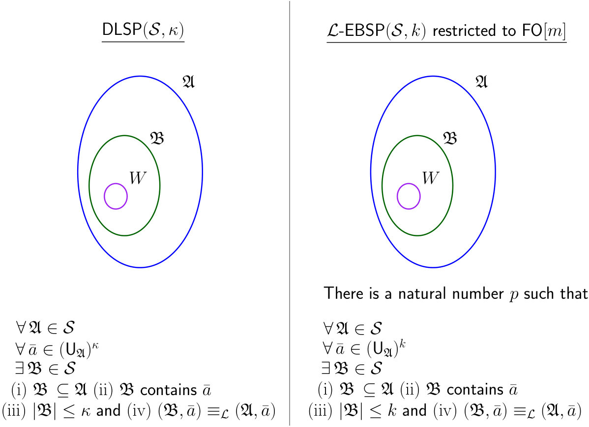 Figure 1
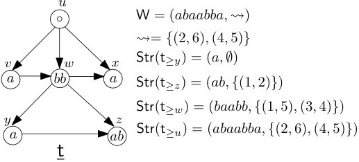 Figure 2