Towards optimal cosmological parameter recovery from compressed bispectrum statistics
Joyce Byun, Alexander Eggemeier, Donough Regan, David Seery, Robert E., Smith

TL;DR
This paper explores compressed bispectrum statistics as proxies to improve cosmological parameter constraints from large-scale structure surveys, aiming to reduce covariance complexity while maintaining information.
Contribution
It demonstrates that modal bispectrum and other proxies can match the Fourier bispectrum's effectiveness with fewer configurations, simplifying analysis without significant information loss.
Findings
Modal bispectrum performs as well as Fourier bispectrum with fewer modes.
Adding bispectrum data improves bias and $\sigma_8$ constraints by up to 5%.
Parameter constraints can improve by up to 20% with bispectrum proxies.
Abstract
Over the next decade, improvements in cosmological parameter constraints will be driven by surveys of large-scale structure. Its inherent non-linearity suggests that significant information will be embedded in higher correlations beyond the two-point function. Extracting this information is extremely challenging: it requires accurate theoretical modelling and significant computational resources to estimate the covariance matrix describing correlations between different Fourier configurations. We investigate whether it is possible to reduce the covariance matrix without significant loss of information by using a proxy that aggregates the bispectrum over a subset of Fourier configurations. Specifically, we study the constraints on CDM parameters from combining the power spectrum with (a) the modal bispectrum decomposition, (b) the line correlation function and (c) the integrated…
Click any figure to enlarge with its caption.
 Figure 1
 Figure 2
 Figure 3
 Figure 6
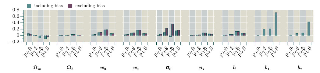 Figure 10
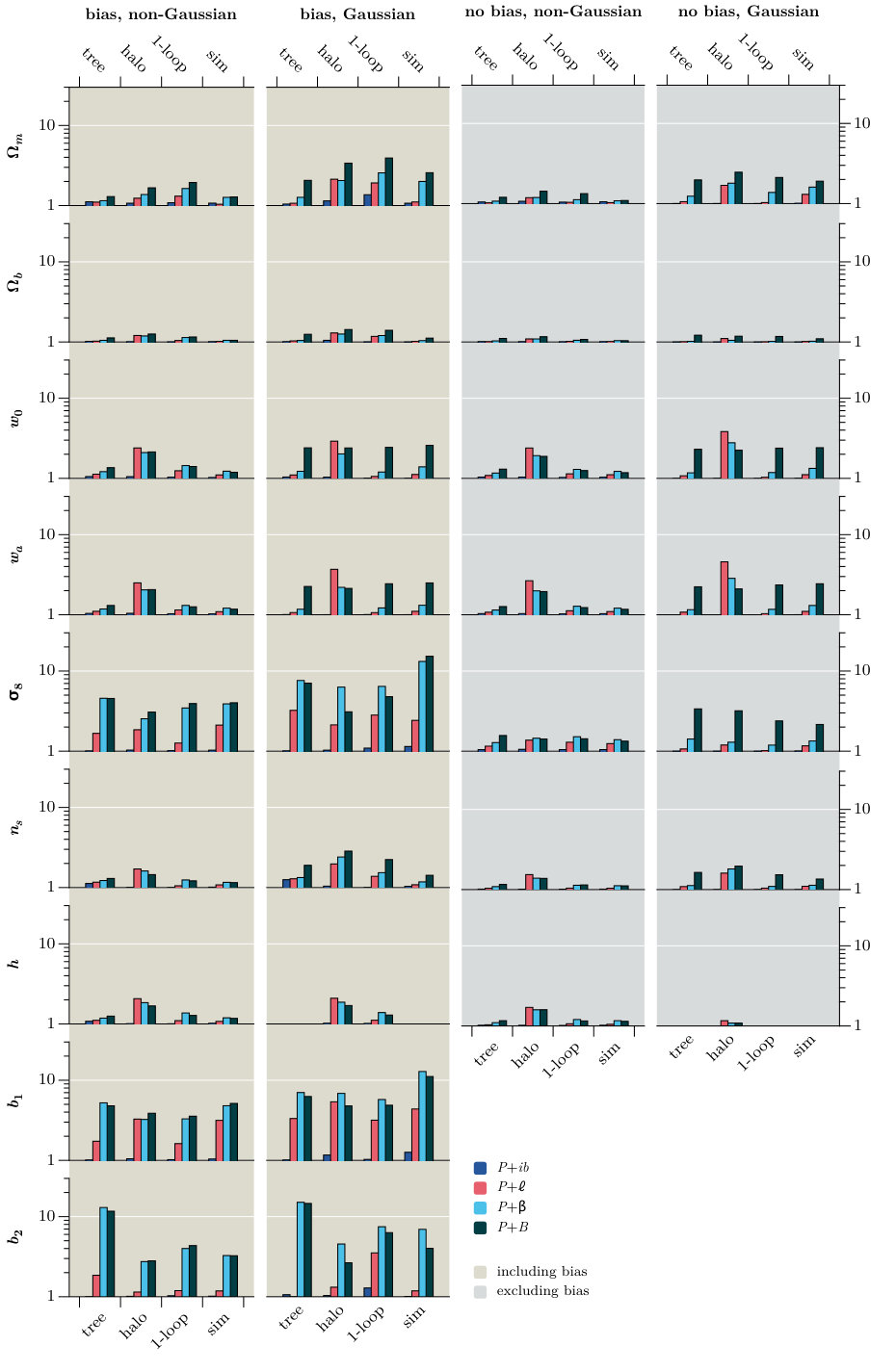 Figure 11
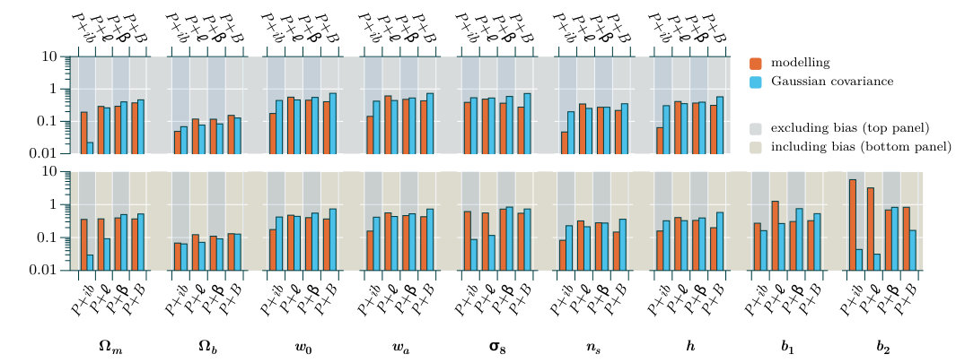 Figure 12
 Figure 13
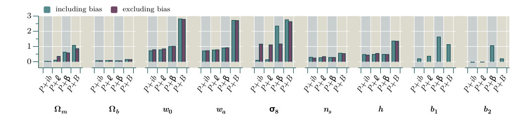 Figure 9
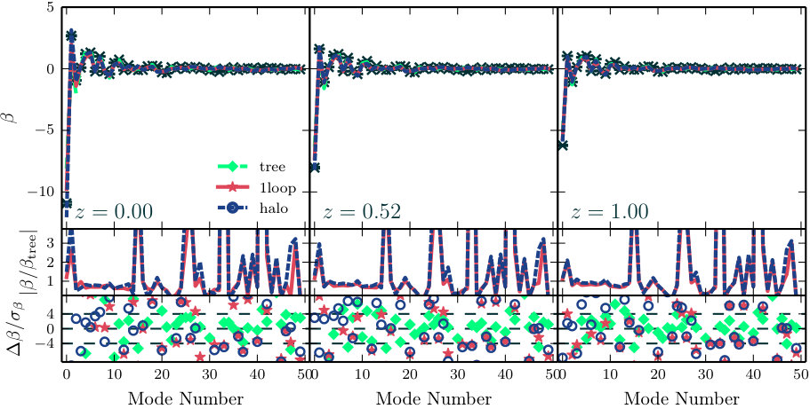 Figure 12
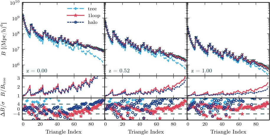 Figure 13
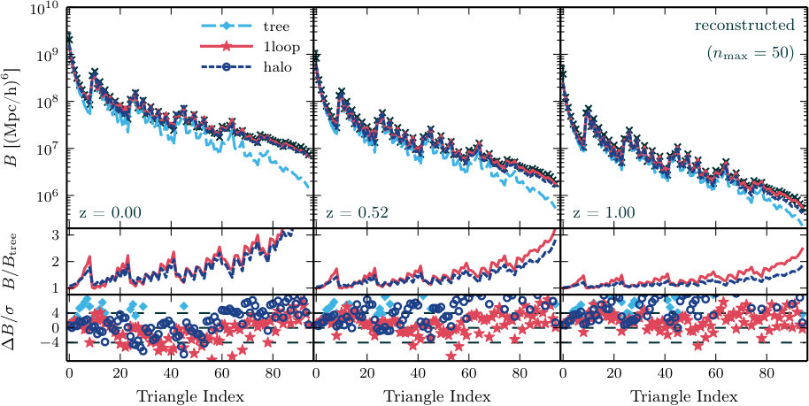 Figure 14
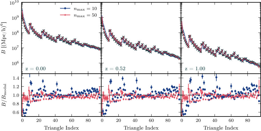 Figure 15
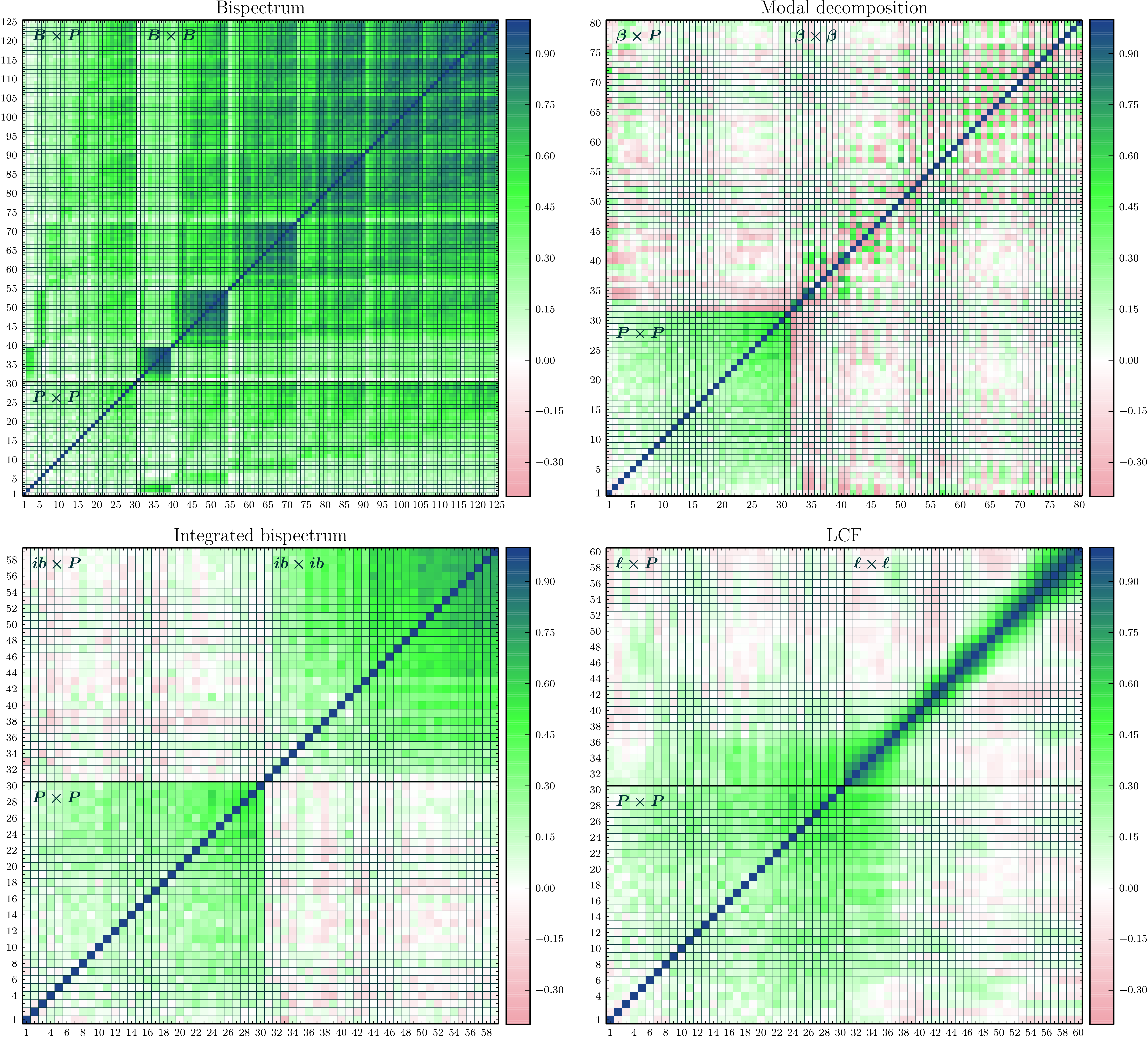 Figure 16
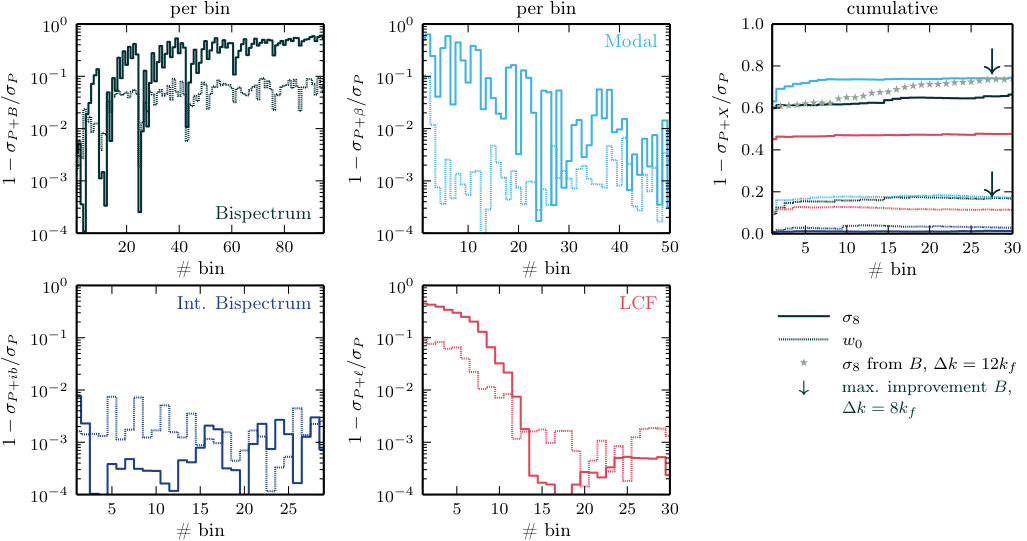 Figure 17
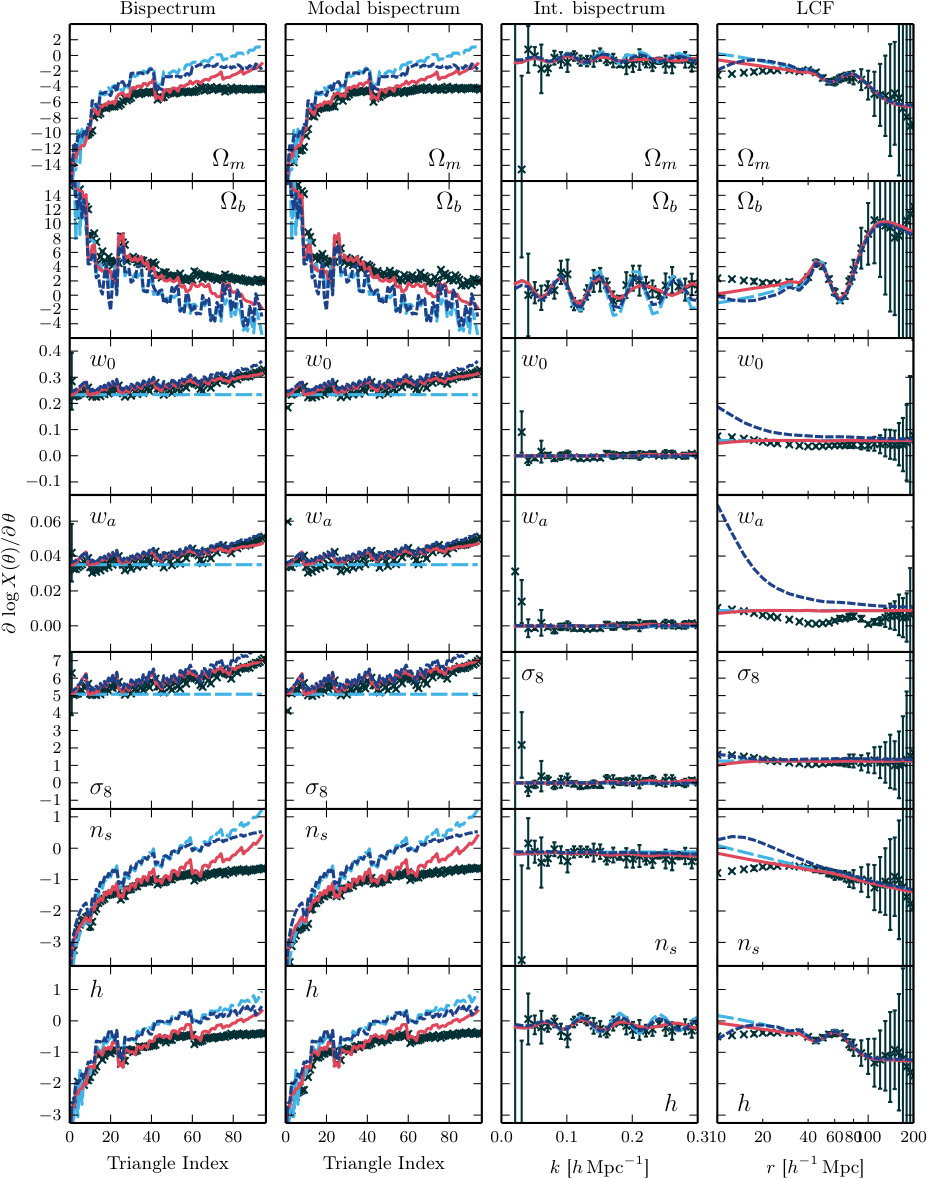 Figure 18
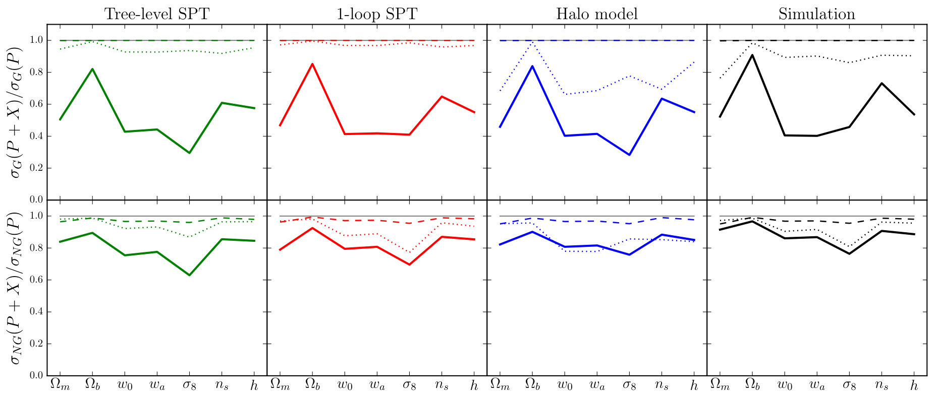 Figure 19
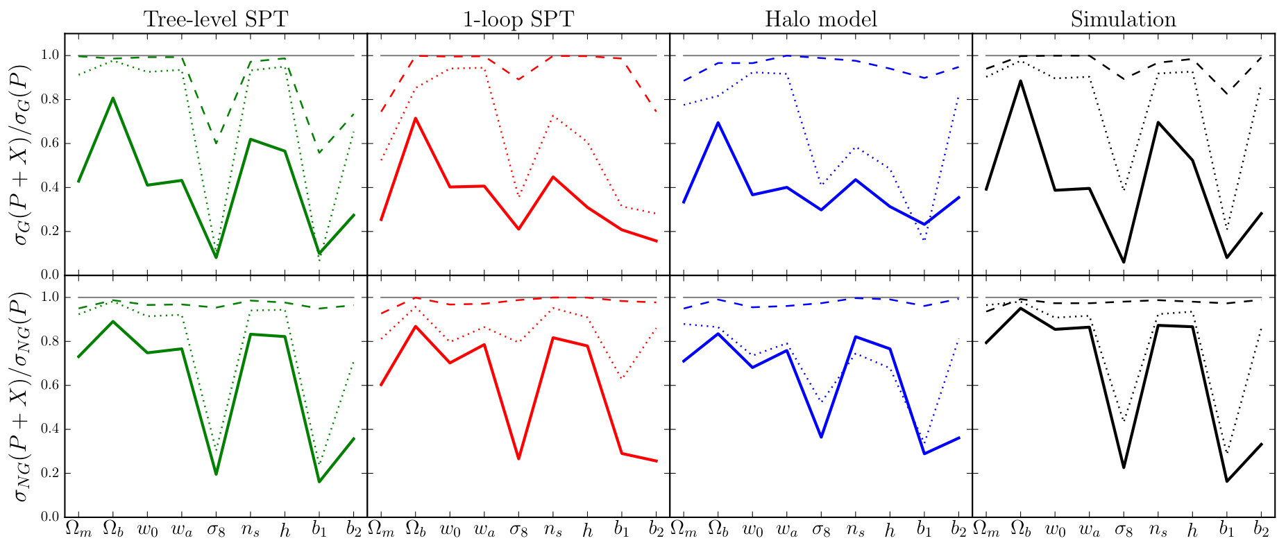 Figure 20
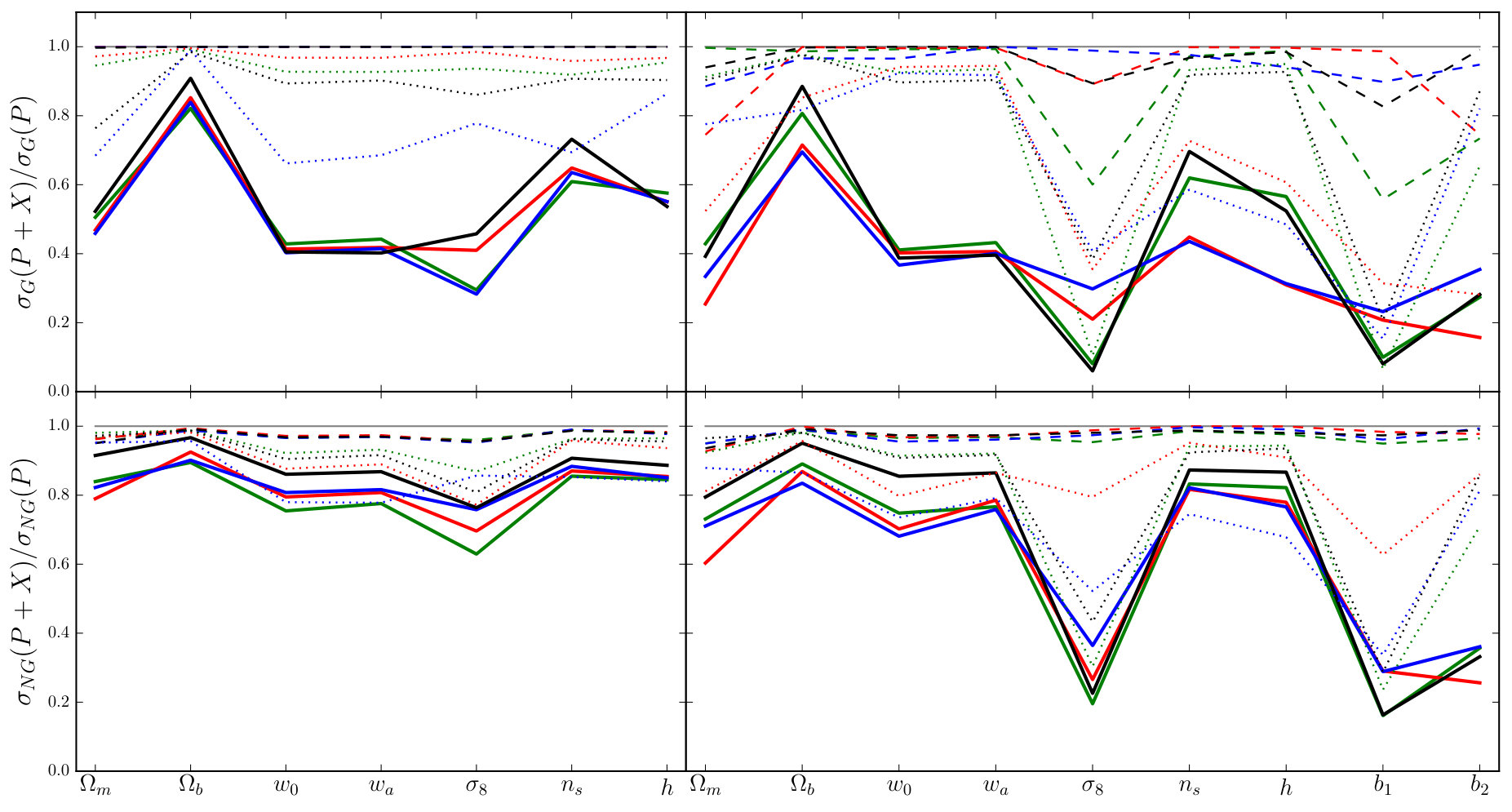 Figure 21
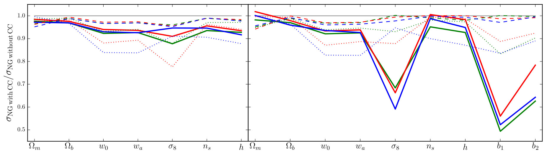 Figure 22
 Figure 23
 Figure 24
 Figure 25
 Figure 26
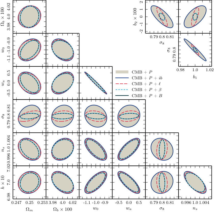 Figure 27
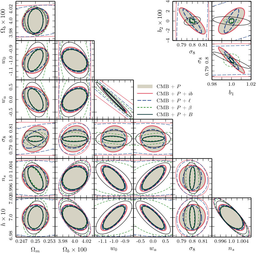 Figure 28
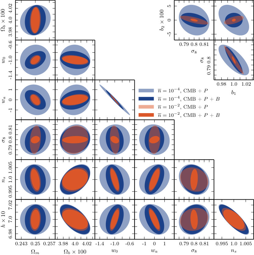 Figure 29
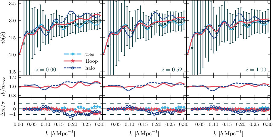 Figure 30
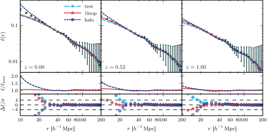 Figure 31
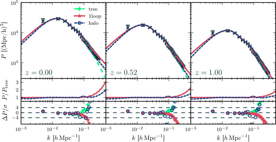 Figure 32
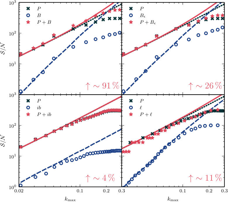 Figure 33
| Parameter | |||||||
| Fiducial value | |||||||
| [] | [] | [] | ||
Peer Reviews
No public reviews on file for this paper yet. If you reviewed it on a platform where reviews are public (OpenReview, ICLR, NeurIPS, ICML), you can paste yours below so the community can read it here.
Videos
No videos yet. Explain this paper in a talk, walkthrough, or lecture? Add one.
Towards optimal cosmological parameter recovery
from compressed bispectrum statistics
Joyce Byun, Alexander Eggemeier, Donough Regan,
David Seery & Robert E. Smith
Astronomy Centre, School of Mathematical and Physical Sciences, University of Sussex, Brighton BN1 9QH, United Kingdom [email protected]@[email protected]@[email protected]
(Accepted XXX. Received YYY; in original form ZZZ)
Abstract
Over the next decade, improvements in cosmological parameter constraints will be driven by surveys of large-scale structure in the Universe. The information they contain is encoded in a hierarchy of correlation functions, and tools to utilize the two-point function are already well-developed. But the inherent non-linearity of large-scale structure suggests that further information will be embedded in higher correlations, of which the bispectrum is currently the most accessible. Extracting this information is extremely challenging: it requires accurate theoretical modelling and significant computational resources to estimate the covariance matrix describing correlations between different configurations of Fourier modes. We investigate whether it is possible to reduce the covariance matrix without significant loss of information by using a proxy that aggregates the bispectrum over a subset of Fourier configurations. Specifically, we study the constraints on CDM parameters from combining the power spectrum with (a) the modal decomposition of the bispectrum, (b) the line correlation function and (c) the integrated bispectrum. We forecast the error bars achievable on CDM parameters in a future galaxy survey that measures one of these proxies and compare them to those obtained from measurements of the Fourier bispectrum, including simple estimates of their degradation in the presence of shot noise. Our results demonstrate that the modal bispectrum performs as well as the Fourier bispectrum, even with considerably fewer modes than Fourier configurations. The line correlation function has good performance but does not match the modal bispectrum. The integrated bispectrum is comparatively insensitive to changes in the background cosmology. We find that the addition of bispectrum data can improve constraints on bias parameters and the normalization by a factor between 3 and 5 compared to power spectrum measurements alone. For other parameters, improvements of up to 20% are possible. Finally, we use a range of theoretical models to explore how the sophistication required for realistic predictions varies with each proxy.
keywords:
Cosmology: theory, Large-scale structure of the Universe
††pubyear: 2017††pagerange: Towards optimal cosmological parameter recovery from compressed bispectrum statistics–LABEL:lastpage
1 Introduction
Constraints on cosmological parameters have improved significantly over the last two decades, driven by high-precision data from the cosmic microwave background (‘CMB’) temperature and polarization anisotropies (Bennett et al., 2003; Ade et al., 2014). But the capacity of CMB observations to sustain this rate of progress is now nearly exhausted. Measurements of the temperature anisotropy have become limited by cosmic variance down to very small scales, and therefore future large-scale measurements will furnish little new information. Meanwhile, on small scales, cosmological information begins to be erased by astrophysical processes. Modest improvements may still come from better polarization data, perhaps shrinking current uncertainties by a factor of a few, but eventually these measurements will also approach the limit of cosmic variance. Further progress will be possible only with new sources of information. In the decade 2020–2030 we expect such a source to be provided by surveys of cosmological large-scale structure—but only if the information these surveys contain can be extracted and understood (Silk, 2016).
**The bispectrum: challenges.—**The statistical information contained in a galaxy survey is carried by its hierarchy of correlation functions, of which typically only a few lowest-order functions can be measured accurately. Tools to extract information from the two-point function were developed early and are now mature. The development of tools to extract information from higher-order correlation functions has proceeded more slowly (Fry, 1984; Goroff et al., 1986; Scoccimarro, 2000; Sefusatti et al., 2006), but because structure formation is non-linear it is likely that these carry an important fraction of the information content. To make good use of our investment in costly observational programmes it will be necessary to find a means of using information from at least the three-point function.
What are the challenges? A first difficulty arises from combinatorics. We write the matter overdensity at time as , where is the density perturbation and is the uniform background. Allowing angle brackets to denote an ensemble average, statistical homogeneity makes the two- and three-point functions and independent of the origin . After translation to Fourier space this enforces conservation of momentum for the wavenumbers that participate in the expectation value,
[TABLE]
where is the common magnitude of the wavenumbers appearing in the two-point function. In Equations (1a)–(1b) and the remainder of this paper we suppress the time labelling the hypersurface of evaluation. Isotropy makes the power spectrum a function only of , while the bispectrum is a function of the three wavenumbers , , subject to the closure condition . Therefore a fixed volume of space yields many more distinct configurations of the bispectrum than of the spectrum. If we choose to measure all of them then we must provide an estimate for their covariance, and beyond the Gaussian approximation this typically requires N-body simulations. Since we require at least as many simulations as the number of independent covariances, the number of simulations to be performed grows at least linearly in the number of configurations. This makes it very expensive to use more than a fraction of the available bispectrum measurements.
Second, we must estimate typical values for in a particular cosmological model. While such estimates are already necessary for the power spectrum , accurate estimates for the bispectrum are substantially more challenging. There are two key reasons. No matter what methods we use, the algebraic complexity associated with high-order correlation functions is usually worse than at lower order. Also, many of our standard tools have a reduced range of validity as we move up the correlation hierarchy. We must therefore work harder to obtain trustworthy predictions from our models, and in some cases we can do so only by giving up analytic methods altogether.
These problems have hampered the development of a toolkit that would make use of bispectrum measurements routine. Nevertheless, they are difficulties of practice and not obstructions of principle—if necessary, we could determine both covariances and typical values of or from N-body simulations, at least over a certain range of scales. But such determinations would require a very large number of realizations. The sheer computational resource entailed by this strategy makes it unattractive on timescales of interest for surveys such Euclid, DESI, or LSST.
**Alternative strategies.—**To build a practical methodology we must cut the size of the covariance matrices and avoid simulations where possible. Simulations are not needed when analytic methods suffice to predict or , or when a Gaussian approximation to the covariance is acceptable. Meanwhile, an obvious way to reduce the number of configurations is simply not to measure them all. Depending how aggressively we choose to cut, this may mean accepting a significant loss of information. A more nuanced option is to aggregate groups of configurations into weighted averages, effectively compressing the data carried by the bispectrum rather than discarding it. Such averages could be computed directly. But there are also observables whose statistics can naturally be expressed as weighted averages of this kind. Measuring these will often be simpler than measuring amplitudes of the Fourier bispectrum—simultaneously reducing the effort required to estimate and invert their covariance matrices. We describe these observables as ‘proxies’ or ‘proxy statistics’ for the full Fourier bispectrum.
Each proxy represents a compromise between (a) information loss due to compression, (b) the type of Fourier configurations over which it aggregates, and therefore the physics to which it is sensitive, and (c) its accessibility to analytical modelling, either for covariances or to estimate typical measurements. In this paper we select three proxies that have already been described in the literature and characterize their performance in each of these categories. Our aim is not to find an optimal proxy for any particular measurement, but rather to demonstrate that their use represents a feasible strategy for upcoming surveys without unacceptable degradation in information recovery.
**Summary.—**Our principal results are forecasts for the parameter error bars achievable from combinations of the galaxy power spectrum and bispectrum, or its proxies. The parameter set we study comprises the background quantities of a CDM model with evolving dark energy, supplemented by two parameters describing the bias model (McDonald & Roy, 2009). We study how these forecasts change when they are estimated using the complete non-Gaussian covariance matrix or its Gaussian approximation. We characterize their dependence on the method used to predict typical values for and by sampling the results using tree-level and one-loop standard perturbation theory (‘SPT’), and an implementation of the halo model. We compare these estimates with values measured directly from simulations. These results can be used to determine, for each observable, the degree of modelling sophistication that is required to obtain accurate forecasts.
Our analysis does not include the effect of survey geometry or incompleteness, or redshift-space effects, and should be regarded as a determination of the performance of each proxy under idealized conditions. We include a simple analysis that indicates how our results would change in the presence of shot noise.
Fisher forecasts including Fourier bispectrum measurements have previously been reported by Sefusatti et al. (2006), assuming bispectrum configurations and measuring covariances from a suite of mock catalogues generated by the PTHalos algorithm (Scoccimarro & Sheth, 2002) and second-order Lagrangian perturbation theory (‘2LPT’). Their results suggested that the bispectrum contains significant cosmological information. For comparison, in our analysis we use bispectrum configurations in order to keep the size of the covariance matrix within plausible bounds, and measure it directly from a suite of full N-body simulations.
More recently, Chan & Blot (2016) estimated the extra constraining power of Fourier bispectrum measurements by computing their contribution to the signal-to-noise, but did not make forecasts for error bars on cosmological parameters. They found that the bispectrum contributed up to a increase in signal-to-noise above the power spectrum and concluded that the information gain would be modest, perhaps being principally useful to break degeneracies. One of our aims is to clarify the relationship between this conclusion and the more nuanced outcomes found by Sefusatti et al. (2006). We find that estimates based on signal-to-noise alone generally give only a rough indication compared to the full Fisher calculation because they do not account for variations in the sensitivity to background cosmology between observables.
**Organization.—**Our presentation is organized as follows. In Section 2 we introduce the three bispectrum proxies to be studied in the remainder of the paper. These are: (a) the modal bispectrum, which can be regarded as an alternative to the Fourier bispectrum obtained by exchanging the Fourier modes for an alternative basis (Fergusson et al., 2012; Regan et al., 2012); (b) the line correlation function, which samples three-point statistics of the phase of the density fluctuation (Obreschkow et al., 2013; Wolstenhulme et al., 2015), and (c) the integrated bispectrum (Chiang et al., 2014), which measures variation of the power spectrum in subsampled regions. Each of these measures can be expressed as a weighted average over particular configurations of the Fourier bispectrum.
In Sections 3.1–3.3 we explain how each proxy can be predicted using the halo model or a flavour of SPT. In Section 3.4 we explain our prescription to obtain the biased galaxy density field from the underlying matter density field, which is the quantity predicted by these analytic models. In Section 4 we describe our procedure to recover estimates for each proxy statistic from N-body simulations, and in Section 5 we compare these estimates (and estimates for their deriatives with respect to the cosmological parameters) with theoretical predictions. Readers familiar with the measures of 3-point correlations described in Section 2 and the modelling technologies of Section 3 may choose to begin reading at this point. In Section 6 we present signal-to-noise estimates for the information content of each proxy. Our Fisher forecasts appear in Section 7. In Section 8 we collect a number of topics for discussion, including the compression efficiency of each proxy statistic and the impact of shot noise on our forecasts. We conclude in Section 9.
**Notation.—**Our Fourier convention is . To avoid confusion we distinguish the Dirac -function or and the Kronecker symbol from the matter overdensity .
2 The Fourier bispectrum and its proxies
In this section we introduce the proxy statistics to which we compare the Fourier bispectrum. This has already been defined—together with the power spectrum—in Equations (1a)–(1b). We describe the integrated bispectrum in Section 2.1, the line correlation function in Section 2.2 and the modal decomposition of the bispectrum in Section 2.3. Each of these represents a possible compression of the Fourier bispectrum, in the sense described in Section 1.
2.1 Integrated bispectrum
The integrated bispectrum (or ‘position-dependent power spectrum’) was developed by Chiang et al. (2014) as a tool to search for primordial non-Gaussianity in large-scale structure. It has several convenient features: it is easily estimated using standard power-spectrum codes and it has a clear physical interpretation. As we shall see in Section 3.1, it represents a weighted average of the Fourier bispectrum dominated by ‘squeezed’ configurations—that is, wavenumbers where one is much smaller than the other two. If we assume then the bispectrum expresses correlations between a single long-wavelength mode and the two-point function . This makes it sensitive to ‘local-type’ non-Gaussianity produced by inflationary models with more than one active field. However, because gravitational collapse correlates modes with comparable wavenumbers, the bispectrum produced during mass assembly is typically concentrated away from squeezed configurations. For this reason it is not clear how sensitive the integrated bispectrum might be to the cosmological parameters that influence this assembly process.
To define the integrated bispectrum divide the total survey volume into cubic subvolumes, each of volume and centred at positions . Compute the power spectrum and average overdensity for each subvolume, which we denote and , respectively. (The power spectrum may depend on the orientation of if the subvolumes are not isotropic.) Finally, the integrated bispectrum is defined to be the expectation of , averaged over the orientation of ,
[TABLE]
The notation indicates that the expectation is to be taken over all subvolumes.
To compute this expectation we Taylor expand in powers of (Chiang et al., 2014). The leading contribution is
[TABLE]
where is the variance in mean overdensity over the subvolumes. Therefore, at lowest order, the integrated bispectrum describes variation of the power spectrum in response to changes in the large-scale overdensity.111In field theory this is the ‘operator product expansion’. We conclude that measurements of contain both the power spectrum and its variance. Since these can be measured directly, any new information contained in the integrated bispectrum must reside in its normalized component (Chiang et al., 2014),
[TABLE]
where the second approximate equality applies when only the lowest-order contribution from the Taylor expansion need be retained. This is the linear response approximation. The quantity is the linear response function and provides a good approximation to for large .
2.2 Line Correlation Function
Equation (1a) shows that the power spectrum is sensitive only to information carried by the amplitude of each Fourier mode. In contrast, higher-order statistics generally encode information carried by both amplitudes and phases. Phase correlations are an exclusive signature of non-Gaussian density fields. For instance, they may arise through processes in the primordial Universe or from mode coupling in the non-linear regime of gravitational collapse. Therefore, unlike the amplitudes, phases directly probe cosmological information that is absent from the two-point function.
With this motivation, Obreschkow et al. (2013) proposed the line correlation function (often abbreviated as ‘LCF’). It measures a subset of three-point phase correlations of the density field—specifically, correlations between collinear points, each separated by a distance . Obreschkow et al. (2013) demonstrated that the LCF is a robust tracer of filamentary structures, and showed that it could be used as a phenomenological tool to distinguish between cold and warm dark matter scenarios. Subsequent work established its connection to conventional higher-order statistics (Wolstenhulme et al., 2015; Eggemeier et al., 2015; Eggemeier & Smith, 2017).
The line correlation function can be understood as follows: for a given density field in some volume , its real-space phase field smoothed on a scale satisfies
[TABLE]
where is the Fourier transform of the smoothing window function. We take this to be a spherical top-hat in -space, , where denotes the Heaviside step function. The phase at is defined so that . Following Obreschkow et al. (2013) the LCF is defined by
[TABLE]
where the factor represents a volume regularization. After taking Fourier transforms we require the three-point function of the in order to evaluate this integral. Wolstenhulme et al. (2015) and Eggemeier & Smith (2017) demonstrated that, at lowest order in the expansion of the probability density function for Fourier phases, this three-point function is directly related to the Fourier bispectrum. Therefore the LCF must contain some fraction of the information in , but because is an average over specific collinear configurations it represents a compression. Specifically, the number of LCF bins will vary linearly with changes in the effective cut-off on Fourier modes.
2.3 Modal bispectrum
Our final proxy is a ‘modal’ expansion of the three-point function. This is very similar to the Fourier bispectrum, except that we exchange the Fourier basis for a set of alternative modes that are better adapted to the structure of . The exchange is helpful if we can represent the bispectrum to the same accuracy using fewer modes than required by the Fourier representation. This approach was originally developed by Fergusson & Shellard (2009) and Regan et al. (2010) to analyse microwave background data, and subsequently applied to large-scale structure by Fergusson, Regan & Shellard (2012) and Regan et al. (2012).
In the alternative basis we represent the Fourier bispectrum in the form
[TABLE]
where the are basis functions that span the space of configurations compatible with a triangle condition on , but can otherwise be chosen freely provided they are linearly independent. The are numbers that we describe as ‘modal coefficients’. They can be regarded as averages of the Fourier bispectrum over a set of configurations picked out by the corresponding . The function is an arbitrary weight that will be chosen in Section 3.3.
If the form a complete basis we expect and to become equivalent in the limit . In this limit the modal expansion is merely a reorganization of the Fourier representation. But if we select the lowest to average over the most relevant Fourier configurations then it may be possible to represent a typical using only a small number of modes.222Here, ‘most relevant’ is defined by the features of the bispectrum for which we wish to search. For example, inspection of the formulae appearing in Sections 3.1–3.2 below shows that both the integrated bispectrum and line correlation function can be regarded as instances of (7), with adjusted to prioritize specific groups of Fourier configurations. For these cases, however, the resulting -basis is not complete. In this paper we distinguish the modal decomposition, for which the -basis is intended to be complete, from proxies such as and which are intended to be projections. Taking to be of order this number, the outcome yields useful compression whenever , where is the number of Fourier configurations contained in the volume under discussion. At least for reasonably smooth bispectra, Schmittfull, Regan & Shellard (2013) found that this could be done with no more than modest loss of signal.
**Orthonormal basis.—**Given a choice of we may redefine the basis by taking arbitrary linear combinations. For example, we will use this freedom in Section 3.3 to obtain a basis for which the -coefficients are uncorrelated. The covariance matrix in this redefined basis is especially simple.
Such a redefinition can be performed using an invertible matrix . We define . The -coefficients in the -basis now satisfy . Since the - and -bases are reorganizations of each other, the modal bispectrum defined using either basis is equivalent,
[TABLE]
3 Predicting typical values and covariances for the proxies
In this section we explain how to obtain predictions for the typical values and covariances of , and in a given cosmological model. This can be done with different degrees of sophistication, corresponding—for example—to truncations at different levels in the loop expansion of standard perturbation theory (Bernardeau et al., 2002), or by using fitting functions calibrated to match the output of N-body simulations (Mead et al., 2015). Since each proxy aggregates a different group of Fourier configurations, and these configurations vary in their response to features of the background cosmology, the sophistication needed to adequately capture the behaviour of the proxies may vary.
This is both a challenge and an opportunity. Proxies that require delicate modelling to obtain accurate predictions are harder to use, and may be expensive to deploy in a parameter-estimation Monte Carlo. In favourable cases, however, the payoff will be sensitive discrimination between nearby cosmological models. On the other hand, proxies that can be modelled robustly using simple methods are easy to use and cheap to deploy, but may offer correspondingly coarse discrimination. We study these trade-offs by contrasting predictions made using tree-level and one-loop SPT, and the halo model. For the halo-model power spectrum we choose the HMcode implementation (Mead et al., 2015). For the halo-model bispectrum we use the standard formulae given by Cooray & Sheth (2002) with a Sheth–Tormen mass function (Sheth & Tormen, 1999) and Navarro–Frenk–White halo profile (Navarro et al., 1996). In Section 5 we study the performance of each method compared to numerical estimates extracted directly from N-body simulations, which enables us to characterize the minimum adequate sophistication for each proxy. For simplicity our analysis is framed in terms of the underlying dark matter density field, although in Section 3.4 we explain how this can be extended to predict galaxy clustering.
**Covariance.—**To compute a likelihood for a given proxy, either for the purposes of parameter estimation or to make forecasts, we require an estimate for the covariance between different configurations. Therefore the minimum sophistication needed to adequately predict this covariance matrix will play an additional role in determining the relative expense of each proxy. In practice the covariance matrix is typically estimated by taking measurements from a large suite of N-body simulations or 2LPT catalogues, or, if this is cannot be done, by falling back to a Gaussian approximation. N-body simulations give accurate results, but are expensive enough that assembling sufficient independent realizations to determine the inverse covariance is often not feasible. In comparison, catalogues based on 2LPT are significantly cheaper but become inaccurate in the non-linear regime, while the Gaussian prediction breaks down even earlier and may miss cross-correlations that significantly affect the outcome.
The relative importance of these cross-correlations varies between proxies. In Sections 6–7 we estimate their significance by comparing results from N-body and Gaussian covariances. We describe our procedure to estimate covariance matrices from the simulations in Section 5, but collect formulae for the Gaussian approximation here.
For comparison, the Gaussian covariance for the power spectrum and Fourier bispectrum, measured on a grid of spacing with fundamental frequency , can be written
[TABLE]
where is the Kronecker symbol, and
[TABLE]
The Kronecker symbol should be interpreted to equal unity if the triangles defined by and are equal, and zero otherwise. The degeneracy factor equals unity for a scalene triangle, two for an isosceles triangle and six for an equilateral triangle.
3.1 Integrated bispectrum
To evaluate the expression (4) we first establish its relation to the underlying 3-point function. The overdensity within the subvolume labelled by can be written
[TABLE]
where is the Fourier transform of the cubic window function with side length , and . The power spectrum in this subvolume is and the mean overdensity is . Combining these with equation (2) yields (Chiang et al., 2014)
[TABLE]
Because is strongly peaked for the window functions effectively constrain the integrals to . Since within each subvolume, the integral receives significant contributions only from squeezed configurations of the Fourier bispectrum that are of order the subvolume size or larger, because in the limit we have .
Chiang et al. (2014) computed the linear response function using (12) and tree-level SPT, and verified that it reproduces equation (4) to within for . For our purposes we require accurate estimates at smaller , and therefore we perform a numerical integration using (12) directly. The integral is 8-dimensional and its evaluation is challenging; we implement it using the Vegas algorithm provided by the CUBA package (Hahn, 2016). To make the integration time feasible we densely sample on a 3-dimensional cubic mesh in coordinates , where is the cosine of the angle between and and can be used in place of the third wavenumber . We construct a 3-dimensional cubic spline that interpolates between lattice points and use this spline to evaluate the integrand. To validate this procedure we have verified that our numerical results match the analytic prediction from the linear response function at large .
Although we have not written subvolume labels explicitly, and all power spectra in (4) refer to subsampled quantities, and therefore should be computed by appropriate convolution with the subvolume window function .
**Halo model.—**This procedure yields good results for tree-level and one-loop SPT, but does not perform well when applied to the halo model. In this case we we do not recover equivalence between our evaluation of (12) and the linear response function, which we compute by numerical differentiation of the HMcode power spectrum. We interpret this disagreement as an indication that the standard halo model makes inconsistent predictions for the modulation of the power spectrum with , or the squeezed limit of the bispectrum, or both. Moreover, comparison of the halo-model computed using (12) to our N-body simulations shows poor agreement, suggesting that estimates based on (12) will be inaccurate. Therefore, for the halo model only, we estimate by assuming the linear response approximation (4) and computing . We calculate the derivative using the simulation-calibrated formula proposed by Chiang et al. (2014),
[TABLE]
which gives reasonable agreement with our simulations.
**Covariance.—**In the absence of shot noise, the Gaussian covariance for estimates of constructed from data can be written
[TABLE]
In this expression is the volume of a subsampled region and denotes the total survey volume. The quantity is the number of Fourier modes in a subvolume -bin.
3.2 Line correlation function
Wolstenhulme et al. (2015) used tree-level SPT to predict the line correlation function. Their result was generalized to an arbitrary bispectrum by Eggemeier & Smith (2017), who gave the formula
[TABLE]
where is the spherical Bessel function of order zero and the integrals over and are cut off at the scale . The quantity is defined by
[TABLE]
and gives the dominant contribution to the bispectrum of the phase field in the limit of large volume . For smaller volumes there are corrections scaling as powers of compared to the dominant term (Eggemeier & Smith, 2017).
**Evaluation.—**To evaluate (15) we must perform a 6-dimensional integral. We use a strategy similar to that described in Section 3.1, by sampling the bispectrum over a cubic lattice and interpolating between lattice sites. The integration is again performed using Vegas.
In the special case of tree-level SPT, Wolstenhulme et al. (2015) showed that (15) could be reduced to a 3-dimensional integral,
[TABLE]
where is the tree-level power spectrum, and the upper limit of the -integral is chosen to guarantee . That requires
[TABLE]
Equation (17) is useful because it provides a means to test the accuracy of our 6-dimensional Vegas integrations, and the 3-dimensional interpolations they entail. We have compared estimates for the tree-level line correlation function using both (15) and (17) and find good agreement.
**Covariance.—**To determine the Gaussian covariance we require the two-point function of the phase field,
[TABLE]
It follows that, in the absence of shot noise, the covariance between estimators for the the line correlation function on scales and can be written (Eggemeier & Smith, 2017)
[TABLE]
where denotes the fundamental frequency (defined above equation (9)), and . Note that (20) is not diagonal; the integral that defines the line correlation function depends on a range of Fourier modes for any scale , and any Fourier modes that are common between and will contribute a nonzero covariance. Moreover, equation (20) shows that the Gaussian covariance is independent of redshift and all cosmological parameters.
3.3 Modal bispectrum
It was explained in Section 2.3 that the modal decomposition is defined by choice of a basis that samples groups of relevant Fourier configurations. The structure and ordering of the determine those configurations we wish to prioritize. But unless we carefully adjust the they will be correlated, and these correlations will be inherited by the . The outcome is that the covariance matrix for estimators of the is rather complex.
**Construction of -basis.—**To avoid this we redefine the basis, as in equation (8), to simplify the covariance matrix for estimators of the corresponding . The construction proceeds in stages. First, consider the expected signal-to-noise with which it is possible to measure a single mode from (7). Using a Gaussian approximation for the noise this can be written
[TABLE]
We are free to choose the weight to simplify this integral. We define
[TABLE]
after which the computation of the expected signal-to-noise reduces to
[TABLE]
To write this and similar expressions economically we have introduced the notation
[TABLE]
for any and . In the special case that these depend only on the wavenumbers and not their orientations some of the angular integrations are trivial and we obtain the simpler expression
[TABLE]
Here, represents the set of points where lines of length , and can be arranged to form a triangle, ie. ; for details, see Fergusson et al. (2010). In principle the integral can be carried over all , but in practice it will be cut off at upper and lower limits and . The expressions (24) and (25) can be regarded as an inner product on the that weights each contributing Fourier configuration according to its individual signal-to-noise.
Second, the -basis is chosen to be diagonal with respect to this inner product. As we will see below, because the resulting modes are orthogonal when weighted by signal-to-noise, the covariance matrix for estimators of the coefficients becomes diagonal under the same approximation of Gaussian noise used to determine the weighting in (21). Specifically, we define
[TABLE]
It is sometimes preferable to express results in terms of , which is independent of and . For any suitable -basis both and will be symmetric and positive-definite and may be factored into the product of a matrix and its transpose. Therefore there exists a matrix such that . Application of (8) with as the transformation matrix yields , and these modes are orthogonal in the sense
[TABLE]
**Determination of modal coefficients.—**Whether we work with the - or -basis, we must predict the corresponding -coefficients for each model of interest. In practice the extra matrix operations needed to obtain the -basis mean that it is simplest to perform calculations in the -basis, before translating to the -basis to interpret the results. We adopt this procedure whenever concrete calculations using the modal decomposition are required. We use the -basis constructed by Fergusson et al. (2010). (The details are summarized in Appendix A.1.) It is not intended to prioritize any single class of Fourier configurations, but rather attempts to provide a good description of reasonably smooth bispectra over a range of shapes and scales.
To extract the we use (24). Assuming (7) can be interpreted as an equality, we conclude that for an arbitrary bispectrum
[TABLE]
Finally, the individual should be extracted by contraction with the inverse matrix . If the bispectrum has no angular dependence then the inner product can be computed using the simplified expression (25), which yields
[TABLE]
where we have used the quantity defined in (16). The may be obtained by the transformation . The appearance of the phase bispectrum in (29) is a consequence of our choice of weight .
Equation (28) would continue to apply were we to change the definition of the ‘inner product’ , and an analogue of (29) would continue to give the individual . Our choice of signal-to-noise weighting in is important only for construction of the -modes and the covariance inherited by the .
**Numerical evaluation.—**In practice, equation (29) requires evaluation of a 3-dimensional integral over the region . To implement it we compute on a cubic lattice in and estimate the integral by volume-weighted cubature over this lattice. Some work is required to account for irregular boundary orientations; we give these details in Appendix A.2.
**Covariance.—**Finally we compute the covariance of estimators for the coefficients under the assumption of Gaussian covariance for the bispectrum estimator . Using equation (24), and (28) with exchanged for , we obtain
[TABLE]
The weighting for each Fourier configuration matches the signal-to-noise, making this correlator diagonal as a consequence of our construction of the -basis. Therefore we conclude
[TABLE]
As for the line correlation function, it is independent of redshift and cosmological parameters. If we were to abandon the approximation of Gaussian covariance then (30) would no longer be proportional to exactly . In this case the amplitude of the diagonal elements would be modified, and non-diagonal components would appear.
3.4 Galaxy bias
The discussion in Sections 3.1–3.3 was framed in terms of the dark matter overdensity , but this is not what is measured by surveys of large-scale structure. Instead, they record the abundance of galaxies or some other population of tracers whose density responds to the dark matter density but need not match it.
On large scales the relation between the galaxy () and dark matter () density fields is well-described by the linear model (Kaiser, 1984; Fry & Gaztanaga, 1993). The linear bias parameter may be redshift-dependent, and varies between different populations of galaxies. On small scales the overdensities are larger, and both non-linear and non-local corrections become important. To obtain a satisfactory description we must typically include terms at least quadratic (or higher) in (Fry & Gaztanaga, 1993; Smith et al., 2007), together with terms involving the tidal gravitational field (Catelan et al., 2000; McDonald & Roy, 2009; Chan et al., 2012; Baldauf et al., 2012).
In what follows we assume the local Lagrangian bias model, in which the galaxy overdensity at early times is taken to be a local function of the dark matter overdensity. At later times the bias is determined by propagating this relationship along the dark matter flow. McDonald & Roy (2009) demonstrated that this implies the Eulerian galaxy overdensity at the time of observation can be written
[TABLE]
where ‘’ denotes terms of third order and higher that we have not written explicitly. The field is a contraction of the tidal tensor, defined by . Therefore, up to second order in , we require two additional redshift- and population-dependent bias parameters: the quadratic bias , as well as the non-local bias . In the local Lagrangian model the non-local bias satisfies (Chan et al., 2012; Baldauf et al., 2012), although in more general biasing prescriptions it could be allowed to vary independently.
**Power spectrum.—**After translating to Fourier space it follows that the tree-level galaxy power spectrum can be written
[TABLE]
To obtain a consistent result at one-loop we should include the unwritten third-order contributions in (32), which generate multiplicative renormalizations of the linear power spectrum in the same way as the ‘13’ terms of one-loop SPT. McDonald & Roy (2009) showed that these could be collected into a single new parameter which we denote to match Gil-Marin et al. (2015). Therefore
[TABLE]
Saito et al. (2014) showed that in the local Lagrangian model satisfies . Explicit expressions for all terms appearing in (34) were given by McDonald & Roy (2009). Note that contributions from the non-linear bias appear only in the one-loop power spectrum.
**Bispectrum.—**In contrast to the power spectrum, the bispectrum receives corrections from non-linear bias terms even at tree-level. Specifically,
[TABLE]
where is the kernel appearing in the Fourier transform of the contracted tidal field, .
To obtain the galaxy bispectrum consistently at one loop one should compute the dark matter overdensity to fourth order in perturbation theory and develop the bias expansion to the same order. This procedure has been adumbrated in the literature (Assassi et al., 2014) but not developed completely. Therefore to obtain an estimate of the one-loop bispectrum we make the approximation
[TABLE]
This is consistent with the prescriptions used by Gil-Marin et al. (2015) and Baldauf et al. (2016).
**Application to bispectrum proxies.—**The outcome of this discussion is that, to predict the integrated bispectrum, line correlation function, or modal bispectrum for the galaxy density field, we should make the replacements and where necessary in equations (12), (15) and (29).
To obtain theory predictions at tree-level we use equations (33) and (35), whereas to obtain perdictions at one-loop we use equations (34) and (36). Finally, to evaluate predictions using the halo model we apply equations (34) and (35), but with and for the dark matter correlations.
4 Estimating bispectrum proxies from N-BODY simulations
In this section we briefly describe our N-body simulations and explain how they are used to estimate the Fourier bispectrum and its proxies , and .
4.1 Simulations
Our measurements are based on two sets of simulations: (1) N-body simulations containing dark matter only, with a fixed choice of fiducial cosmological parameters; (2) a total of simulations constructed by varying one cosmological parameter at a time, with four realizations per model including the fiducial set. These simulations were performed on the ZBOX supercomputer at the University of Zurich and were described in Smith (2009) and Smith et al. (2014). Each set uses a comoving boxsize of and contains particles. Initial conditions for the particles were set at redshift using second-order Lagrangian perturbation theory acting on a realization of a Gaussian random field (Crocce et al., 2006) with transfer functions from CMBFAST (Seljak & Zaldarriaga, 1996). The particles are evolved to under the influence of gravity using the Gadget-2 code (Springel, 2005), modified to allow a time-evolving equation of state for dark energy.
The fiducial cosmological parameters correspond to a flat CDM model and are summarized in Table 1. Specifically, and are the matter and baryon density parameters; and parametrize the equation of state for dark energy, viz. ; is the amplitude of density fluctuations smoothed on a scale ; is the spectral index of the primordial power spectrum; and is the dimensionless Hubble parameter. We collectively write these as a vector with index labelling the different parameters. To construct set (2) each parameter is offset by and , with all other parameters held fixed. The stepsizes are listed in Table 1. To reduce noise when estimating parameter derivatives, we construct initial conditions for each of the four realizations using the same Gaussian random field as its fiducial partner. Since we vary over seven cosmological parameters this gives a total of simulations in the suite.
4.2 Density field
To compute the overdensity field in each simulation we use the cloud-in-cell assignment scheme to distribute particles over a regular Cartesian grid. We apply a fast Fourier transform and extract the discrete real-space density field by deconvolving the cloud-in-cell window function. The result is
[TABLE]
The labels ‘disc’ and ‘grid’ label Fourier-space fields in the full volume and on the cloud-in-cell grid, respectively. The Nyquist frequency is determined by the number of grid cells per dimension. For our numerical results we use .
4.3 Estimating the power spectrum
Given a realization of the -field within a simulation volume , a simple estimator for the power at wavevector can be written .333In the remainder of this paper we assume it is understood that we are dealing with the discrete density field whenever we refer to measured quantities, and drop the label ‘disc’. Unfortunately this procedure is very noisy. An improved estimate can be obtained by summing over a set of modes satisfying the closure criterion within a thin -shell. Since we are working in finite volume the available modes are discretized in units of the fundamental frequency , and therefore the thin-shell average should be written
[TABLE]
where represents a bin width, and we have introduced the binning function which is defined to be unity if and zero otherwise. Finally, the quantity represents the volume of the spherical shell accounting for discretization,
[TABLE]
4.4 Estimating the bispectrum
In analogy with the power spectrum, an estimator for a single configuration of the Fourier bispectrum can be written . [This expression was already used in Section 3.3 to obtain the Gaussian covariance for estimators of the .] To obtain an acceptable signal-to-noise we should again average over a set of configurations whose wavenumbers lie within suitable discretized -shells. After doing so we obtain the estimator
[TABLE]
where the normalization should now be evaluated using (Sefusatti et al., 2006; Joachimi et al., 2009)
[TABLE]
Dividing by the square of the fundamental cell volume shows that the number of configurations scales as , where is the length of the side in units of the fundamental mode. Hence, if we scale the configuration by then the number of available configurations scales as .
Sefusatti (2005), Fergusson, Regan & Shellard (2012) and Scoccimarro (2015) observed that (40) could be implemented efficiently by rewriting the Dirac -function using its Fourier representation, , and factorizing the dependence on the . This yields
[TABLE]
Similarly,
[TABLE]
where is the inverse Fourier transform of .
Equation (42) is numerically more efficient than a direct implementation of (40), because it requires only three Fourier transforms to compute for each wavenumber in the triplet . Moreover, once each has been obtained it can be re-used for any configuration that shares the same wavenumber. In spite of this improvement, however, it remains a formidable computational challenge to estimate all bispectrum configurations contained within a large volume . Different strategies have been employed to make the calculation feasible. One option is to coarsely bin configurations with binning width equal to several times the fundamental mode. This drastically reduces the number of configurations to be measured. An alternative is to search only among a limited subset of configurations. This may be helpful if we wish to search for specific physical effects, but risks overlooking important signals if we are searching blindly. In either case the analysis is unlikely to be optimal because information is lost.
4.5 Estimating the integrated bispectrum
Our procedure to estimate the integrated bispectrum is based directly on its definition. We separate the total volume into subvolumes, enumerated by the labels . We compute the mean overdensity and power spectrum within each subvolume. Finally, we average the product over all subvolumes. Therefore,
[TABLE]
The normalized integrated bispectrum can be obtained by rescaling,
[TABLE]
where here is the average subvolume power spectrum and is the average variance of the mean overdensity.
4.6 Estimating the line correlation function
A procedure to estimate the line correlation function was outlined by Eggemeier & Smith (2017). We evaluate
[TABLE]
where denotes an average of taken over the volume of a fundamental -space cell centred at . The sum scales as , making its evaluation fast on large scales but challenging on small ones, where the sum includes the majority of Fourier modes. On scales below we find that the real space estimator described by Eggemeier & Smith (2017) becomes more efficient and therefore we use it within that regime. For scales accessible to both schemes we verified that both estimators yield the same result.
4.7 Estimating the modal bispectrum
Equation (29) shows that an estimate of the modal coefficient requires evaluation of , where is the bispectrum estimator defined in Section 4.4. Using equation (24), writing the -function using its Fourier representation, and factorizing the integral as described in Section 4.4, we find
[TABLE]
Here, is a polynomial used in the construction of the modes ; see Appendix A.1. Equation (47) shows that the computation can be reduced to a single 3-dimensional integral over the , which are themselves weighted Fourier transforms of . Finally, can be estimated by contracting with the inverse inner product matrix defined in (26),
[TABLE]
To obtain the corresponding -basis coefficients requires a further linear transformation
[TABLE]
where is the matrix defined above (27). As explained in Section 3.3, we generally perform numerical calculations in the -basis in order to preserve the simplicity of (47), but present results in the -basis because their covariance properties make these coefficients simpler to interpret. In either basis, the measured coefficients can be used to reconstruct the bispectrum for any required Fourier configuration using equation (8).
Note that, because the matrix can be tabulated, measuring a single modal coefficient has the same computational complexity as measuring a single configuration of the Fourier bispectrum.
4.8 Choice of bins
In Table 2 we summarize the parameters used in implementing estimators for each of these statistical quantities. The power spectrum and Fourier bispectrum are binned by averaging over shells of width as explained in Sections 4.3–4.4. For the same reasons we also average the subvolume power spectra used to construct the integrated bispectrum. The line correlation function and modal coefficients do not involve averaging over shells, but instead are evaluated using equations (46) and (47) which are themselves aggregates over groups of configurations. For each statistic we report the minimum and maximum -modes that contribute, and the total number of measurements or bins. Note that the bispectrum bin width corresponds to .
In what follows we will label the Fourier configurations for the bispectrum using the scheme of Gil-Marin et al. (2016). We assign the label (or ‘index’) zero to the equilateral configuration with . The remaining configurations are ordered so that and . Their labels are assigned by sequentially increasing , and (in this order) and incrementing the index for each valid triangle.
In our measurements of the integrated bispectrum we split the simulation box into subcubes, corresponding to a side of . This increases by a factor of five compared to the full box. Finally, for the line correlation function we use a non-regular -spacing, spanning the range from to . The first seven bins are separated by , which doubles to for the next eleven and to for the remaining twelve bins.
5 Comparison of theoretical predictions and simulations
In this section we present estimates of the typical values for each bispectrum proxy introduced in Section 2, and implemented using the formulae of Section 4. We derive these from the 200 simulations of our fiducial cosmology in set (1)—see Section 4.1—at redshifts , and . Also, using the simulation set (2) we determine how each proxy responds to changes in the cosmological parameters (Section 5.2). These measurements enable us to characterize the accuracy of the theoretical predictions for these typical values discussed in Section 3. Finally, in Section 5.3 we discuss measurements of the covariances and cross-covariances for each pair of proxies.
5.1 Mean values in the fiducial cosmology
5.1.1 Comparison of measurements and theoretical predictions
In Figs. 1–4 we show measurements of each proxy for all three redshifts, averaged over the different realizations. We do not explicitly display our power spectrum measurements, which have been well-studied by previous authors (e.g. Makino et al., 1992; Lokas et al., 1996; Scoccimarro & Frieman, 1996; Scoccimarro et al., 1998; Scoccimarro et al., 2001; Smith et al., 2003; Seljak, 2000; Peacock & Smith, 2000; Scoccimarro & Sheth, 2002; Mead et al., 2015). In each figure, the top row contrasts our N-body measurements with the tree-level, one-loop and halo model predictions. The middle row displays the one-loop and halo model predictions relative to the tree-level prediction, and the bottom row shows the difference between the N-body measurements and the theoretical prediction in units of the standard deviation of the N-body estimate.
**Fourier bispectrum.—**We find that both of the SPT predictions are more accurate at large scales and high redshifts. The halo model prediction is a better match at low redshift. The differences between each theoretical estimate and the typical values measured from simulation are broadly consistent with previous analyses; see Scoccimarro et al. (1998); Scoccimarro et al. (2001); Schmittfull et al. (2013); Lazanu et al. (2016).
**Modal bispectrum.—**In Fig. 2 we plot the Fourier bispectrum reconstructed from (7) using our measurements of the coefficients. This is easier to interpret than the -values themselves. The scatter between predicted and measured values (most clearly visible in the bottom row) is similar to the scatter for the directly-measured Fourier bispectrum (Fig. 1), and indicates that differences between the reconstructed and directly-measured values are small. We give a more detailed analysis of the accuracy of the modal bispectrum in Section 5.1.2.
**Integrated bispectrum.—**We give values for the normalized integrated bispectrum in Fig. 3. Except for a few -bins the error bars are too large to show any preference for a particular theoretical model. In contrast to Figs. 1–2, the bottom row shows that tree-level SPT is a good match to the measured at all three redshifts. Conversely, the halo model prediction is a better match at high redshift. Our theoretical predictions are consistent with those reported by Chiang et al. (2014), but our measured values have larger error bars because we work with a smaller simulation volume.
**Line correlation function.—**Finally, we present our measurements of the line correlation function in Fig. 4. The one-loop and halo-model predictions appearing here are new, and have not previously been studied. The most striking feature is the discrepancy between the halo model and SPT-based predictions in the smallest -bins. This is consistent with the analyses of Wolstenhulme et al. (2015) and Eggemeier & Smith (2017), which both found differences between the tree-level prediction and values measured from simulation on scales with . The agreement is good for larger .
**Theory error.—**The bottom panels of Figs. 1–4 show that our theoretical predictions are accurate within a restricted range of scales. Outside this range it becomes progressively more difficult to model the observables. This mis-modelling should be regarded as an additional source of systematic error—a theory error—when forecasting constraints, or analysing data, using any of these theoretical models. In particle phenomenology such theory errors are routinely estimated when performing fits to data, but their use in cosmology is less common. In this paper we construct Fisher forecasts for parameter error bars using both SPT-based models and the halo model. Comparison of these error bars enables us to estimate the impact of theoretical uncertainties on future constraints that incorporate three-point statistics (see Section 7.4).
An alternative prescription for estimating theory errors was used by Baldauf et al. (2016) and Welling et al. (2016). In their approach the theoretical uncertainty in one-loop SPT is estimated from the next-order term in the loop expansion. We find that this prescription gives noticeably larger estimates than the difference between one-loop SPT and the values we measure from simulations. Therefore, although Baldauf et al. (2012) and Welling et al. (2016) concluded that (for example) constraints on some types of primordial non-Gaussianity would be weakened significantly after accounting for theory errors, our numerical comparison suggests that the attainable error may degrade by less than their analysis would suggest.
5.1.2 Accuracy of modal reconstruction
Comparison of Figs. 1 and 2 demonstrates that the Fourier bispectrum reconstructed from our measurements of the accurately reproduces the correct amplitude and shape dependence. This information is embedded in the modal coefficients. For example, the zeroth basis mode is a constant and therefore captures information about the mean amplitude of the Fourier bispectrum over all configurations—or, equivalently, the skewness of . The next few modes are slowly varying functions of configuration. Taken together, these low-order modes carry the principal amplitude information and for reasonably smooth bispectra we expect they exhibit the strongest dependence on background cosmological parameters. The higher modes capture more subtle detail. As with any basis decomposition, their inclusion increases the accuracy of the reconstruction.
To see this in detail, consider a reconstruction using only modes. In Fig. 5 we plot the Fourier bispectrum reconstructed in this way (blue line) compared to the reconstruction using described above (red line). Black crosses mark the measured data points. In the lower panel we plot the ratio between these measured values and the reconstructions. The accuracy is good whether we use or , but the scatter is smaller for . We conclude that, in this case, the first 10 modes are sufficient to capture the main behaviour of the Fourier bispectrum, but extra modes are helpful if we wish to reproduce the precise configuration dependence to within accuracy.
5.2 Derivatives with respect to cosmological parameters
In the remainder of this paper our aim is to obtain Fisher forecasts of error bars for a parameter set , where the index labels one of the cosmological parameters of Table 1. For this purpose the role of a theoretical model is to predict the derivatives of observables with respect to each parameter, and the accuracy of the forecast depends on the reliability of these predictions. In this section we study how well our three theoretical models reproduce the derivatives estimated from our simulation suite. We compute the derivative of some estimator at wavenumber with respect to a parameter by the rule
[TABLE]
where is the average over the fiducial simulations of set (1) (described in Section 4.1) for , and the logarithmic derivative with respect to is computed using
[TABLE]
The sum is over the four realizations used in simulation set (2), and the derivative is constructed using the and offset simulations described in Section 4.1. The advantage of the logarithmic derivative is that both realizations in the numerator on the right-hand side of (51) share initial conditions with their fiducial partner in the denominator. Therefore, division by the fiducial estimate minimizes dependence on the specific realization.444This strategy is less successful for the line correlation function. In this case the fiducial value could be very close to zero on some scales. In turn, this produces large errors in the logarithmic derivative. Therefore, for the line correlation function, we estimate the linear derivative instead.
In Fig. 6 we plot the derivatives of each observable with respect to the cosmological parameters at . Our forecasts use three redshift bins, but their behaviour is similar to the bin and the statements made below can be taken to apply at all three redshifts. We do not include the power spectrum, for which the derivatives appeared in Smith et al. (2014).
**Modal bispectrum.—**To simplify comparison of the modal bispectrum with the Fourier bispectrum, Fig. 6 plots derivatives of the reconstructed bispectrum rather than derivatives of or . Comparison of the first two columns shows that the cosmology-dependence is accurately captured using , either for theoretical predictions or the measured values.
There is a significant spread in performance of the theoretical models, with tree-level SPT and the halo model generally offering the poorest match. For the derivatives with respect to , , and these models give similar predictions. The probable reason is that, in the standard halo model, the halo mass function and halo profile are fixed to the fiducial cosmology. Only the input power spectrum is taken to vary with the cosmological parameters, and since it matches the tree-level SPT prediction its derivatives will be equal. Therefore the halo-model derivatives will differ from those of tree-level SPT only via a (possibly scale-dependent) prefactor. More complex halo models with cosmology-dependent halo parametrizations have been studied (see, eg., Mead et al. (2016) for an application to dark energy models). However, determining which variation of the halo model captures the cosmological parameter dependence of the bispectrum most accurately is outside the scope of this paper. We simply note that, if the halo model is to be used for analysis or forecasting of the Fourier bispectrum, its implementation should be chosen with care because its performance depends on these details.
**Integrated bispectrum.—**The derivatives of the integrated bispectrum are shown in the third column of Fig. 6. The errors bars on the measured values are again too large to show a clear preference for any model—and they are generally so large that the measurement is not significantly different from zero. These results are consistent with those reported by Chiang (2015) for a range of values of , and . We conclude that the integrated bispectrum is rather insensitive to the background cosmology and is therefore a comparatively poor tool to constrain it. While this means we must expect a Fisher forecast to predict weaker error bars for the parameters of Table 1, this insensitivity could be an advantage if the intention is to use the integrated bispectrum as a probe of other physics. For example, in addition to the background cosmology we may wish to use the large-scale structure bispectrum to constrain the possibility of primordial three-point configurations produced by inflation on squeezed configurations. Insensitivity to the background cosmology would reduce the likelihood of degeneracies in these measurements.
**Line correlation function.—**The last column of Fig. 6 shows the derivatives of the line correlation function. As for the typical values discussed above, the values predicted by our theoretical models are significantly discrepant with the measured values in the smallest bins. Also, the derivative with respect to the dark energy parameter is particularly discrepant for the halo model. One possible explanation is the construction of the halo model as described above, with its fixed halo mass function and halo profile. Alternatively, it is possible that the halo model power spectrum and bispectrum that we use are subtly inconsistent in a way that produces inaccuracies in the line correlation function on small scales.
5.3 Non-Gaussian covariance
The analytic, Gaussian covariance of each proxy is most accurate at high redshifts and on large scales, where the matter fluctuations are more nearly Gaussian and therefore more accurately described by the power spectrum alone. At low redshifts and on small scales, however, the Gaussian approximation fails due to non-linear evolution of matter fluctuations. This evolution generates additional contributions to the covariance through higher-order -point correlations.
The simplest and most robust approach to obtain accurate non-Gaussian covariances has been to analyse large suites of N-body simulations. This method was used by Takahashi et al. (2009), Takahashi et al. (2011), Blot et al. (2016), and Klypin & Prada (2017) to study the non-Gaussian covariance of the power spectrum. Other authors have performed analogous studies for the bispectrum (Sefusatti et al., 2006; Chan & Blot, 2016), the real-space partner of the integrated bispectrum (Chiang et al., 2015), and the line correlation function (Eggemeier & Smith, 2017). In this section, we present our measurements of the non-Gaussian covariance for each proxy, estimated from our suite of simulations. We also discuss the cross-covariance between pairs of proxies.
In Sections 6 and 7 we quantify the impact of these complex non-diagonal covariances on estimates of signal-to-noise and Fisher forecasts.
**Correlation matrices.—**We plot correlation matrices for the measurements , , , and in Fig. 7. We show measurements only at where differences between the Gaussian and non-Gaussian covariances are largest.
The correlation coefficient between two data bins and is defined to satisfy , where is the covariance matrix estimated from the simulation suite,
[TABLE]
and is the number of realizations. To measure an auto-covariance the data vector contains all measurements of a single proxy, or to measure a cross-covariance it contains all measurements from a pair, , where . The correlation matrix measures the degree of coupling between different measurements. Its elements take values between (where the bins are fully anti-correlated) and (where the bins are fully correlated). A value of zero corresponds to independent measurements. For comparison, the Gaussian covariance matrices for , , and are diagonal, whereas for there are correlations between neighbouring bins with similar because it is a real-space statistic and therefore includes contributions from many Fourier configurations. In the Gaussian approximation the cross-covariance between and any bispectrum proxy is zero.
**Fourier bispectrum.—**For (upper-left panel of Fig. 7) the correlation matrix has an approximate block structure due to the ordering of the 95 triangle configurations that we measure. The blocks correspond to groups of adjacent configurations with shared values of or . While the power spectrum shows mild correlations between different bins at high , the bispectrum exhibits much stronger correlations. There are also non-zero cross-correlations between power spectrum and bispectrum bins. The correlation between power spectrum and bispectrum tends to be higher when and have wavenumber bins that overlap. Similarly, the correlation between different bispectrum bins is higher when the configurations share at least one wavenumber. However, even configurations that have no wavenumbers in common can be strongly correlated, with correlation coefficient as large as , due to non-linear growth.
**Modal bispectrum.—**In the upper-right panel of Fig. 7 we present measurements of the correlation coefficients for . These have not previously been reported. As explained in Section 3.3 these measurements apply to the -basis, for which the covariance matrix is constructed to be diagonal in the Gaussian approximation. We find that only the first two modes are correlated with the majority of bins. This is reasonable because the lowest modes probe the most scale-independent features of the phase bispectrum. The remainder show low-to-moderate correlation or anti-correlation due to non-linear effects.
**Integrated bispectrum and line correlation function.—**Correlation measurements for the integrated bispectrum appear in the lower-left panel of Fig. 7. The measurements show stronger auto-correlations than as increases, while the cross-correlation is relatively featureless. This indicates that the two data sets are nearly independent. Similarly, we find that the cross-correlation is nearly featureless except where the smallest bins and highest bins show significant correlation. Relative to the Gaussian covariance matrix for , the bins with are more strongly correlated due to non-linear growth.
**Cross-covariances.—**Finally, we have computed the correlation matrices between the bispectrum and its proxies. These enable us to identify which bispectrum configurations contribute most to individual bins of , or . We find that the first two modes are strongly correlated with the bispectrum over large range of triangles, while the remainder are generally more correlated with triangles on the largest scales (that is, lower triangle index). This structure is similar to the correlation matrix.
We find that and are very weakly correlated, which we attribute to being dominated by more strongly squeezed triangles than any we include in the 95 measured configurations of . Finally, the line correlation function is correlated with a majority of bispectrum configurations when . This indicates that the line correlation function is sensitive to many different shapes of Fourier triangle. We do not find particularly strong correlations for , but shows that the line correlation function at small is highly correlated with the first two modes. This is consistent with the observation that both are sensitive to a wide range of Fourier configurations.
6 Cumulative signal-to-noise of the bispectrum proxies
Before discussing the constraining power of each proxy we first compute the available signal-to-noise. This is an intermediate step that characterizes the significance with which measurements of each proxy can be extracted from a data set. Negligible signal-to-noise would normally imply poor prospects for parameter constraints. For example, Chan & Blot (2016) and Kayo et al. (2013) studied the signal-to-noise as a proxy for the information content of the Fourier bispectrum in the context of large-scale structure and weak lensing, respectively.
**Numerical procedure.—**The cumulative signal-to-noise up to a maximum wavenumber is defined by
[TABLE]
where is the vector of typical values for either a single proxy or a combination of proxies, defined below equation (52). In this and subsequent sections we drop the use of a hat to denote an estimated value, and an overbar to denote a mean. The sum in (53) runs over all bins containing wavenumbers that satisfy the condition . For the Fourier bispectrum a bin corresponds to a triplet of wavenumbers , all of which are required to be smaller than .
We use the non-Gaussian covariance matrix measured from simulations, described in Section 5.3, which we denote by . Its inverse is not an unbiased estimator of . A simple prescription to approximately correct for this bias is to rescale by an Anderson–Hartlap factor (Anderson, 2003; Hartlap et al., 2006), which yields
[TABLE]
where is the number of realizations used to estimate the covariance matrix and is its dimensionality.555Although the Anderson–Hartlap prescription is simple to apply, it has been pointed out by Sellentin & Heavens (2016) that this rescaling simply broadens the Gaussian likelihood of the data. These authors argued that the distribution of the data is more accurately modelled by a -distribution. Care should be taken when computing the numerical inverse , especially for combinations of measurements with signals of widely disparate magnitude. To avoid issues associated with ill-conditioning we first compute the correlation matrix , whose entries lie between and . We determine the inverse using a singular value decomposition and check that all singular values are above the noise. Finally, we compute the inverse covariance using
[TABLE]
**Results.—**In Fig. 8 we plot the resulting signal-to-noise measurements for the Fourier bispectrum, integrated bispectrum, line correlation function and the quantity defined in (16) and used in the construction of the line correlation function and the modal bispectrum. (The signal-to-noise from and the reconstructed modal bispectrum give almost identical results.) We estimate using the prescription
[TABLE]
Each panel of Fig. 8 shows the cumulative signal-to-noise of the Fourier bispectrum or a proxy (blue circles), together with the power spectrum (black crosses) and their combination including the cross-covariance matrix (red stars). The first four data points in the and panels use a bin size in order to probe the low- regime. The remainder derive from the measurements presented in Section 5 and use . Our measurements of the integrated bispectrum and line correlation function carry forward the binning procedure used in Section 5. The step-like structure that occurs for is due to a mismatch of scales between the power spectrum and the bins of the line correlation function. In each panel, for comparative purposes, we plot lines of matching colour to show the signal-to-noise computed using a Gaussian approximation to the covariance matrix and tree-level SPT to evaluate any correlation measures it contains.
**Discussion.—**First, we note that the Gaussian approximation overpredicts the signal-to-noise for each proxy and its combination with the power spectrum. This is consistent with the results reported by Chan & Blot (2016). The overprediction occurs because bins become coupled by non-linear evolution, and therefore do not provide independent information as the Gaussian approximation assumes. The effect can be quite severe: while the power spectrum signal-to-noise at is overpredicted by a factor of three, the impact on the Fourier bispectrum and its proxies is much larger. In these cases the overprediction ranges from a factor of or for and up to more than an order of magnitude for the Fourier bispectrum. At smaller the overprediction is less, becoming significant for .
The Fourier bispectrum, phase bispectrum, and line correlation function individually contribute of the signal-to-noise of at , while the integrated bispectrum achieves only of the signal-to-noise. For the Fourier bispectrum, this result is consistent with Chan & Blot (2016).
However, for estimating parameter constraints from the joint combination of and , or one of its proxies, the individual signal-to-noise contributed by one of these measurements is less important than whether it contains information that is not already present in the power spectrum. This is determined by the signal-to-noise of the combination compared to alone. The different proxies show significant variation in the improvement from use of , which we indicate as a percentage in the bottom-right corner of each panel. Although , and individually carry roughly the same signal-to-noise, the uplift in varies from to . Note that the signal-to-noise of receives a large improvement from the cross-covariance, which was ignored in Chan & Blot (2016).
The discrepancy in uplift between and is striking. If this discrepancy were to carry over to parameter constraints it would imply that the Fourier bispectrum carries significantly more constraining power than , even though both statistics are equivalent in the approximation of Gaussian covariance. If true, this would be very surprising. We return to this question in Section 7.5 after we have obtained forecast parameter uncertainties for and its proxies, which enable us to precisely quantify the constraining power of each statistic.
7 Parameter uncertainty forecasts
In this section we collect our major results, which are Fisher forecasts of the error bars achievable on the parameter set of Table 1, based on a fiducial flat CDM cosmology. We perform these forecasts with and without inclusion of the bias parameters .
In Section 7.1 we summarize our implementation of the Fisher forecasting method, and in Section 7.2 we present and compare the forecasts from each proxy. By comparing forecasts with and without non-Gaussian covariances, and using different theoretical models to describe the dark matter density, we are able to characterize their influence on the final parameter constraints. These discussions appear in Sections 7.3 and 7.4, respectively. Finally, we return to the discussion of Section 6 and examine to what extent the signal-to-noise provides a reliable metric by which to estimate improvements in parameter constraints (Section 7.5).
7.1 Forecasting method
The Fisher formalism can be used to forecast the precision with which cosmological parameters could be measured in a future survey. Consider a data vector containing measurements of any combination of statistical quantities. The likelihood function is defined to be the probability of the data given the parameters , so . Then the Fisher matrix satisfies
[TABLE]
The expected error on each parameter , marginalized over all other parameters, can be obtained from the diagonal elements of the inverse Fisher matrix using . To simplify the computation of we make the assumption that the likelihood function is a multivariate Gaussian,
[TABLE]
where denotes a matrix transpose and is the determinant of . We have written the mean of the data vector as , and its covariance matrix is . With these assumptions it can be shown that (Tegmark et al., 1997),
[TABLE]
The first term measures variation of the covariance matrix with respect to the parameters, which is often a smaller effect than the variation of the means represented by the second term. In the approximation that this first term may be neglected the Fisher matrix can be computed in terms of the inverse covariance matrix for the fiducial model. Our procedure to obtain this matrix from the simulation suite has already been described in Sections 5 and 6.
**Survey configuration.—**The Fisher formalism depends explicitly on details of the survey under discussion, both through the specification of the data vector —such as how many redshift bins are used and which Fourier configurations are included—and the properties of the covariance matrix . In the following we adopt the parameters of an idealized survey of large-scale structure consisting of three independent redshift slices at , and . Each slice has volume and a mode cutoff at . The total Fisher matrix can be written as a sum of the Fisher matrix in each slice,
[TABLE]
We assume that, in each redshift bin, the number density of galaxies is sufficiently high that the effect of shot noise is small. We do not include redshift-space distortions or the effect of complex survey geometry. In general, all of these effects will be significant for a realistic survey and cannot be neglected. However, in this paper our intention is to address the question of whether the proxies described in Section 2 can be competitive with measurements of the Fourier bispectrum in principle. Survey-specific effects will generally reduce the number of configurations that can be measured, or increase the noise on those for which measurements are possible. This will typically weaken the performance of the proxies, meaning that their neglect gives us an estimate of the best-case scenario. While we do not anticipate that astrophysical or observational systematics will affect any one proxy more than the others, this is an interesting question to explore in future.
Each of the constraints we present includes a prior from the cosmic microwave background power spectrum. We implement this prior by adding a fourth Fisher matrix,
[TABLE]
Details of the computation of for our choice of fiducial parameters were given by Smith et al. (2014).
7.2 Constraining power of the bispectrum and its proxies
In this section we present our forecasts. To minimize modelling errors we construct the Fisher matrix for each proxy using quantities measured from simulation, except for derivatives with respect to the bias parameters which cannot be obtained in this way. For the Fourier bispectrum we compute these derivatives analytically by differentiating the one-loop power spectrum (34) and the tree-level bispectrum (35). Once the derivatives have been obtained we replace occurrences of the dark matter power spectrum and bispectrum with their measured values. Our prescription for the proxies is similar, using the one-loop power spectrum to estimate derivatives of and tree-level formulae together with the formulae of Section 3 to estimate derivatives of the proxy.
We plot the forecast confidence contours in Fig. 9. Each panel shows predicted joint constraints for a pair of parameters after marginalizing over all the others. The grey shaded region marks the constraint predicted from measurements of the power spectrum only, except for inclusion of the CMB prior that we apply to all estimates. The solid dark-blue line marks the constraint predicted from ; the long-dashed red line marks the constraint predicted from ; the short-dashed light-blue line marks the constraint predicted from ; and the solid black line marks the constraint predicted from . We summarize the marginalized error bars in Table 3. The value in parentheses following each uncertainty indicates the percentage improvement compared to use of alone.
**Improvement from three-point correlation data.—**First consider the joint constraints from (solid black lines in Fig. 9). These demonstrate that substantial improvements can be achieved compared to measurement of the power spectrum only. This is especially evident for and the two bias parameters, for which the improvement is roughly –; compare the second column of Table 3. This is perhaps unsurprising: the bispectrum constrains a different combination of and than the power spectrum, and therefore assists in breaking their degeneracy (Fry, 1994; Matarrese et al., 1997). Nevertheless, other parameters that do not participate in this degeneracy also experience improvements in the range –, with the exception of . This is already very well-measured by the CMB prior, and large-scale structure measurements can add little new information. These conclusions are similar to those reported by Sefusatti et al. (2006), who suggested that inclusion of Fourier bispectrum measurements could reduce uncertainties on and by a factor in the range to .
Next, the forecast for the integrated bispectrum (solid dark-blue lines) shows that it offers negligible improvement, of order , in comparison to alone. This is consistent with the very small dependence on cosmological parameters discussed in Section 5.2, and the low signal-to-noise obtained in Section 6. On the other hand, the line correlation function offers comparable constraints to the Fourier bispectrum for and , which receive improvements of and , respectively. Eggemeier & Smith (2017) demonstrated that this occurs because the line correlation function is nearly independent of and therefore probes a different direction in parameter space than or . Also, inclusion of measurements increases sensitivity to the dark energy parameters and by . These improvements are only marginally degraded compared to those from , which are of order .
Finally, Fig. 9 demonstrates that the modal bispectrum with (short-dashed light-blue lines) is predicted to yield error bars nearly equivalent to the Fourier bispectrum with triangles. Note especially that there is no sign of the significant difference in constraining power between and —which is the quantity implicitly measured by with our choice of basis—that was suggested by our analysis of signal-to-noise in Section 6. We return to this apparent discrepancy in Section 7.5 below. Just as important, the differences between the cases and are mostly negligible. Therefore, even with as few as modes, the modal decomposition retains nearly the full constraining power of the bispectrum. However, it should be remembered that Fig. 5 suggests the Fourier bispectrum reconstructed with so few modes will introduce more significant scatter. In a realistic analysis, these reconstruction errors could manifest themselves as a bias on the best-fit cosmological parameters. Unfortunately we cannot account for this bias in our Fisher analysis, but it deserves further investigation.
**Combination with other observables.—**The strong degeneracy between and can be broken by other means. For example, it is possible to use weak lensing measurements that probe the matter power spectrum directly. Given that inclusion of 3-point correlation data yields the largest improvements for and the bias, it is worthwhile considering what improvements should be expected were the bias to be fixed by other cosmological observations.
In a scenario of this kind the power spectrum constraints would not be weakened by marginalization over the bias parameters, and therefore inclusion of 3-point correlation data would no longer yield such a dramatic improvement for . However, we still find encouraging improvements for many parameters. For example, inclusion of either Fourier or modal bispectrum measurements would decrease uncertainty on by and all other parameters except by –. Inclusion of measurements would decrease uncertainty on by , on the dark energy parameters by , and for all other parameters by . We conclude that, even in the extreme case that and can somehow be determined exactly, inclusion of 3-point correlation data still provides valuable additional information.
These Fisher forecasts should be interpreted with some care. As explained above, we do not include a number of astrophysical and observational effects that complicate the analysis of realistic galaxy survey data. These include redshift uncertainties, redshift-space distortions, irregular survey geometries and shot noise. In particular, for the forecasts presented here the effective shot noise is set by the number density of particles in our simulation suite. This is substantially larger than the galaxy number densities that will be achieved by upcoming surveys. We return to this issue in Section 8.2, where we discuss how our predictions would be modified by a more realistic number density.
7.3 Effect of non-Gaussian covariance and cross-covariance
The non-Gaussian covariance measured in simulations differs from the Gaussian approximation in two ways: (1) it includes additional contributions to the variance of each bin from higher-order correlations, and (2) it adds or enhances coupling between different bins of a single proxy, and between bins of different proxies. These non-Gaussian corrections generally lead to weaker parameter constraints when compared to forecasts constructed using the Gaussian approximation, because this assumes that every bin contributes independent information. In this section we compare the relative impact of non-Gaussian covariance for the different proxies by contrasting Fisher forecasts made with and without its inclusion. We give results for the combinations , , and and each choice of theoretical model—tree-level SPT, 1-loop SPT, or the halo model.
**Increase in uncertainty from non-Gaussian contributions.—**Fig. 10 shows the relative increase in predicted uncertainty for each parameter when non-Gaussian contributions are included. To estimate we use the expressions for Gaussian covariance given in Section 3 with each quantity replaced by its value measured from our simulations. For example, to construct the Gaussian covariance for we use equation (14) with replaced by its measured value. We could equally well have constructed similar estimates using one of the theoretical models to calculate such values, but the result is not very different. The discussion in this section would continue to apply if we were to reproduce Fig. 10 using estimates generated by any of these prescriptions.
The increase in uncertainty induced by inclusion of non-Gaussian effects depends on the measure of 3-point correlations used to generate constraints, the method used to estimate the Gaussian covariance matrix, and the parameter in question. In general we find that the Gaussian approximation underpredicts the uncertainty for the Fourier bispectrum more strongly than for its proxies. Note also that—although and yield nearly identical constraints when the non-Gaussian covariance is used, as described in Section 7.2—the importance of the non-Gaussian covariance for these combinations is not the same. Since the quantity measured by is not the same as , neglecting cross-covariance with (as the Gaussian covariance does) will leave out different information for compared to .
Inclusion of non-Gaussian covariance impacts uncertainties for , and more significantly than the other parameters. This non-uniformity means that it is not obvious how inclusion of non-Gaussian covariance might impact constraints from 3-point correlations on further parameters not considered here. For instance, a number of authors have used Gaussian covariances to forecast future constraints on a primordial bispectrum generated by inflation; see Scoccimarro et al. (2004), Sefusatti & Komatsu (2007), Sefusatti et al. (2012), Baldauf et al. (2016), Welling et al. (2016) and Tellarini et al. (2016). It is not yet clear how these forecasts will change when more realistic non-Gaussian covariances are used.
**Inclusion of cross-covariance.—**In Fig. 11 we summarize the influence of cross-covariance between and the 3-point measures by comparing constraints using the full non-Gaussian covariance to constraints where the cross-covariance has been set to zero. We find that inclusion of cross-covariances reduces the predicted uncertainties for nearly all parameters and choices of combination , whether or not we marginalize over galaxy bias. In the few cases where inclusion of cross-covariance did not reduce the uncertainties (e.g. constraints on from and ), the predicted error bar is weakened by less than 12% of the error bar without cross-covariance. Overall, we find that ignoring cross-covariances can overestimate uncertainties by up to when we do not marginalize over the bias, and by for the special case of bispectrum constraints on the bias parameters themselves.
This reduction of uncertainties due to inclusion of cross-covariances may be surprising. While we have not explicitly identified the source of the improved constraining power, this is not a new feature of Fisher forecasts using non-Gaussian covariances. For example, a number of authors using cross-correlations between cluster counts, weak lensing power spectra and the weak lensing bispectrum have found that parameter constraints can improve when cross-covariances between strongly-coupled measurements are included (Takada & Bridle, 2007; Sato & Nishimichi, 2013; Kayo et al., 2013). But it is also possible that our improvements are partly due to the galaxy biasing model we have chosen. A simulation of halos, rather than dark matter alone, could be used to verify the effect when simultaneously constraining both cosmological parameters and galaxy bias.
The conclusion of this discussion is that an accurate estimate for the covariance matrix, including non-Gaussian contributions and off-diagonal terms, is important if we wish to obtain reliable constraints. Unfortunately, this is especially true for the Fourier bispectrum for which the Gaussian approximation most significantly underestimates the true parameter uncertainties. This implies that surveys aiming to generate constraints from inclusion of measurements cannot evade the computational difficulties associated with estimating their covariance matrix.
To mitigate these difficulties we could consider use of rather than . As we have seen in Section 7.2, these combinations yield nearly equivalent constraints using Fourier configurations and modal coefficients respectively, and therefore the modal decomposition makes the information content of the bispectrum more accessible by reducing the size of the covariance matrix needed to obtain it. We consider the efficiency with which each proxy can compress the information carried by in Section 8.1.
7.4 Theory-dependence of the forecasts
In Section 7.2 we have presented our Fisher forecasts based on simulated data, and in Section 7.3 we have discussed the influence of non-Gaussian covariance and cross-covariances. These results enable us to assess the information content carried by the Fourier bispectrum and its proxies, but the question of how easily these statistics can be deployed remains open. In particular, we would like to know whether the use of simulated data is essential, or whether any of the models described in Section 3 are sufficient. In this section we study the dependence of our forecasts on the choice of theoretical model used to estimate the derivatives in equation (59).
**Match to forecast from simulations.—**First, we consider whether there is a model that provides a clear best-match to the forecast using simulated data. Fig. 12 compares the forecasts for each parameter using different prescriptions for the covariance matrix and for different choices of theoretical model, with marginalization over the bias included or excluded. The bar heights represent the reduction in the predicted uncertainty provided by a given combination, relative to the base model of power spectrum data only combined with a CMB prior. The results of Section 7.2 are labelled ‘sim’. Unfortunately, for each combination there is no single choice of theoretical model yielding forecasts that provide the best match to the ‘sim’ outcome for all parameters—with or without marginalization over bias.
For example, consider the combination in the first column of Fig. 12. This summarizes forecasts generated by including non-Gaussian covariance and marginalization over the bias. For it is 1-loop SPT that gives the best match to the ‘sim’ result, but for the linear bias parameter the best match comes from tree-level SPT.
Alternatively, one could ask whether any one model provides uniformly conservative or uniformly optimistic forecasts. If so, that model could be used to estimate upper or lower limits on the uncertainty for any chosen parameter. But Fig. 12 demonstrates that there are no models with such properties. For example, focusing again on the first column, there is no single choice of theoretical model for that forecasts the largest or smallest improvement for all parameters.
**Sensitivity to theory error.—**Next, we study the variation in forecasts for the Fourier bispectrum and its proxies when we change the model used to compute . To understand the sophistication required to obtain accurate models we will need to understand which of these statistics (if any) are especially sensitive or immune to theoretical mis-modelling. We measure this dependence by a sensitivity factor, which we define to be the ratio between the largest and smallest forecast uncertainties taken over the models of Section 3. A sensitivity factor close to unity indicates that a forecast uncertainty depends only weakly on the choice of theoretical model, while a large value indicates that the model has a strong influence on the final outcome.
We plot these sensitivity factors in Fig. 13, computed with inclusion of all bias parameters and using non-Gaussian covariances. Therefore the sensitivity factor solely reflects the variation in uncertainty produced by different choices for theoretical model. We conclude that there is no single measure of 3-point correlations that consistently yields the largest or smallest sensitivity to variations in modelling. Therefore, there is apparently no single combination that should be preferred to minimize the effect of theory errors on inferred parameter constraints.
**Ranking by constraining power.—**Neither of these criteria provide a rationale to prefer a choice of theoretical model. Nevertheless, we do find some general trends. Irrespective of theoretical model, we find the largest reductions in parameter uncertainties when the bias is constrained simultaneously with the cosmological parameters. Also, the Fourier bispectrum and modal bispectrum consistently offer the most significant improvements compared to -only measurements, with very similar predicted uncertainties. The line correlation function achieves moderate improvement compared to -only, while the integrated bispectrum has very weak constraining power—at least for the parameter set we consider. We conclude that or should be preferred for constraints on CDM parameters, with offering similar information at reduced computation cost as discussed at the end of Section 7.3.
**Relative importance of modelling and non-Gaussian covariance.—**Finally, we consider the relative importance of non-Gaussian covariance and theoretical modelling for obtaining quantitatively accurate forecasts. In Fig. 14 we show the fractional difference in Fisher forecasts induced by variation of theoretical model (orange bars) and use of the Gaussian approximation (blue bars). To quantify the significance of theoretical modelling we plot , where . Therefore larger orange bars reflect more significant deviation from the simulated forecast due to theoretical uncertainty. Meanwhile we quantify the role of the covariance matrix by plotting , so increasing blue bars show that the Gaussian approximation generates more significant errors in the forecast.
Fig. 14 shows that the impact of theoretical uncertainty for and is generally less significant than neglect of non-Gaussian covariance, whether or not we marginalize over the bias. In contrast, for the effect of modelling nearly always dominates because of the difficulties with the halo model discussed in Section 5.2. For the non-Gaussian covariance plays an important role if the bias parameters are not included, but theoretical modelling dominates when they are.
On balance, these results indicate that our forecasts are slightly less sensitive to theory error than to the approximation of Gaussian covariance. This could be because the inverse covariance weighting suppresses contributions from the non-linear regime where the theoretical predictions are most discrepant. But the difference is not large: the average variation in our predicted uncertainties from and due to theory modelling is , whereas the variation due to Gaussian covariances is . Therefore, we conclude that both issues must be addressed in order to obtain quantitatively accurate results.
7.5 Signal-to-noise as a proxy for the information content
It is now necessary to address the question of why the large discrepancy in uplift between the signal-to-noise of and (equivalently ) observed in Section 6 did not translate into significant differences in the forecast for parameter uncertainties in Section 7.2.
Consider a vector of values combining measures and of the 2- and 3-point correlation data, respectively, as defined below equation (52). For a given parameter the reduction in uncertainty compared to measurements from alone can be estimated in the Fisher framework by
[TABLE]
To avoid ambiguity we use the notation to denote the covariance matrix of the power spectrum only. Meanwhile, the increase in signal-to-noise in the same scenario is given by
[TABLE]
The uplift in signal-to-noise is often taken as an approximation to the reduction in parameter uncertainty, which avoids the need to compute . As we have seen in Section 5.2, these derivatives can be rather fragile and are susceptible to significant errors caused by theory mis-modelling. Unfortunately, when applied to and our analysis demonstrates that the ratios and are nearly equal, whereas the same ratios constructed using are very discrepant. Therefore we must conclude that improvements in signal-to-noise cannot always be interpreted as a predictor of the improvement in Fisher information.
**Invariance of the Fisher matrix.—**First consider the Fisher matrix. Suppose we perform a redefinition so that , where may be an arbitrary nonlinear function of the original measurements. For example, the transformation from to is of this type. The derivative transforms ‘contravariantly’ on its index , in the sense . Meanwhile, the covariance matrix becomes
[TABLE]
where ‘’ denotes terms involving higher order correlations that we have not written explicitly. Provided these are small compared to the term, equation (64) shows that the covariance matrix also transforms ‘contravariantly’, and therefore that its inverse transforms ‘covariantly’. Subject to these approximations we conclude that the Fisher matrix should be roughly invariant. This agrees with our observation that and are nearly equal, demonstrated numerically in Table 3.
Now consider the signal-to-noise. Since has neither a co- or contravariant transformation law, the combination appearing in the signal-to-noise will typically not be invariant. Therefore different choices and may yield inequivalent results for . For example, we have verified that using predicts a significant increase in the signal-to-noise compared to , whereas their Fisher matrices continue to agree. In Table 4 we summarize the improvement in unmarginalized constraints from the addition of or . This demonstrates that empirically the increase in signal-to-noise from provides a more accurate estimate of the Fisher information than . This property holds for both proxies of , namely the modal bispectrum, and the line correlation function.
**Gaussian limit.—**This outcome is not inconsistent with the result that and show an equivalent uplift in signal-to-noise in the Gaussian approximation. In this case the covariance matrix for is , where the constant takes the values , or for scalene, isosceles and equilateral configurations, respectively, as described in Section 3. In the same approximation the covariance matrix for the Fourier bispectrum is . Therefore we conclude that the signal-to-noise for and is identically equal as
[TABLE]
In the Gaussian approximation the power spectrum is an independent source of information, which explains the agreement. However, once off-diagonal contributions in the covariance matrix are included, and are no longer independent and non-linear combinations may give very different results for the signal-to-noise.
**Comparison with Chan & Blot.—**Our signal-to-noise for differs from that reported by Chan & Blot (2016) because we include cross-covariance (Section 6). Since empirically the signal-to-noise of gives a more accurate estimate of the information gain from 3-point correlation data, the expected improvement from the 3-point information in is in good agreement with the improvement suggested by Chan & Blot (2016). However, the details of these calculations are rather different. The unmarginalized constraints in Table 4 and most of the marginalized constraints in Table 3 support this conclusion. For , and , for which the effect in Table 3 is substantially larger than , we ascribe the improvement to degeneracies of that are broken by 3-point correlation data.
8 Discussion
8.1 Compression and efficiency of the Fourier bispectrum proxies
In an ideal survey aiming to measure the Fourier bispectrum we should clearly choose a bin width that is sufficiently small to reproduce all small-scale features of interest. However, because the number of Fourier configurations in a volume with mode cut-off scales as this task will quickly become computationally expensive. And, as we have emphasized several times, a more serious problem is that we must estimate and invert the covariance matrix for all these measurements. This requires us to perform at least as many N-body simulations as the number of configurations that we retain.
In this section we consider how well this large number of Fourier configurations can be compressed by the proxies described in Section 2. Suppose that available resources limit the number of simulations that can be performed in such a way that we can estimate an accurate covariance matrix for bins of the Fourier bispectrum or one of its proxies, in combination with another measurements of the power spectrum . Among the measures of 3-point correlations that we consider, is there a preferred choice that provides optimal constraints on our set of cosmological parameters? If so, this measure would provide the most successful compression of the full Fourier bispectrum into a manageable number of measurements.
**Compression by reduction to bins.—**To this end we combine the power spectrum bins with a single additional configuration from the Fourier bispectrum or one of its proxies, and compute the corresponding Fisher matrix (as in Section 7.1) using values for estimated from our simulation suite. The four left panels of Fig. 15 show the reduction in predicted uncertainty—defined as the shrinkage of the error bar, —for the representative parameters (solid lines) and (dotted lines) for each of the possible bins. Using these reductions as a measure of the information stored in each bin we conclude that most of the information carried by the Fourier bispectrum is contained in small-scale triangles (towards larger triangle index). A similar conclusion applies for the line correlation function, for which significant reductions occur only for the first bins, corresponding to the range of scales – . This is reasonable, because the line correlation is constructed to give a negligible signal on large scales. Finally, while the modal decomposition exhibits some variability, smaller mode numbers typically provide larger gains. The integrated bispectrum shows consistently weak improvements over all bins.
Second, for each combination we identify a set of bins for that provide the largest improvements. Adding them cumulatively to the power spectrum, starting from the bin carrying most information, we obtain the plot on the right-hand side of Fig. 15. Both the line correlation function and the modal bispectrum converge rapidly to the maximal improvement available from the entire set of bins that we measure (this is bins for and modes for —see Table 2). For example, the line correlation is already within of the maximum after we have added bins, while only modes of are required to arrive at a similar value for the modal bispectrum. In comparison the Fourier bispectrum converges much more slowly to the maximum provided by the bins that we measure. This is especially evident for , for which the improvement from the Fourier bispectrum has not yet converged to its maximum value after the bin. (For guidance, we mark this maximum value with black arrows on the plot.) However, it should be noted that our procedure to select the set of bins is not optimal because it does not account for covariances between them. By analysing random subsets of the possible bispectrum bins we find that faster convergence is possible, giving up to of the maximum reduction after bins.
**Compression by broadening bins.—**Rather than reducing the number of configurations by restriction to a subset, we might alternatively increase the width of each bin. The same volume of data would then be compressed into fewer measurements. To compare the performance of this strategy we repeat the analysis described above for the Fourier bispectrum with a broader bin width , which gives rather than Fourier configurations with . We plot the corresponding cumulative reduction in uncertainty for as star-shaped symbols in the right-hand panel of Fig. 15. After bins the improvement is similar to that obtained from the modal bispectrum, with the same caution about rate of convergence due to correlation between bins. Therefore—rather surprisingly—in this case we find no clear preference for the bin width or , except that is more computationally expensive, and it is more difficult to find an optimal subset of configurations. However, it is not clear whether this conclusion would survive in a more realistic analysis, where the signal can be noisy and demands finer binning. To explore these issues in detail would require a more comprehensive analysis.
**Results.—**This analysis agrees with the conclusions of Sections 7.3 and 7.4, and supports the modal bispectrum as a good choice of proxy for 3-point correlation data. In addition to the advantages discussed in previous sections, it requires the fewest bins and loses almost no information.
These results could be modified in cases where it is possible to compute a covariance matrix for configurations of the Fourier bispectrum, as done (for example) by Gil-Marin et al. (2016). However, the mock catalogues used to produce such covariance matrices are often generated using perturbation theory and therefore are likely to be inaccurate on small scales. We expect that it is a better strategy to use fewer bins and obtain high-quality measurements of the covariance matrix from catalogues generated using full N-body simulations. The significant benefit of the modal decomposition is that it facilitates construction of the smallest set of bins that still carry a majority of the information.
Finally, although the line correlation function provides weaker improvements than either the Fourier bispectrum or modal bispectrum, it has the advantage that it clearly separates the scales carrying useful information from those that do not—all bins with have negligible impact. It is also possible that the performance of the line correlation function could be improved by relaxing the condition of strict collinearity, which would increase the range of Fourier configurations it is able to aggregate.
8.2 Shot Noise
Galaxies are discrete, point-like tracers of the underlying matter fluctuations, and therefore samples of their abundance are affected by shot noise. This noise is expected to impact higher-order statistics more significantly than the power spectrum (Sefusatti & Scoccimarro, 2005; Chan & Blot, 2016). Up to this point our analysis has implicitly used the low effective shot noise provided by our simulations, and therefore there is some concern that our forecasts will degrade with larger, more realistic noise. In this section we perform an approximate analysis of this degradation and quantify its effect on our predicted parameter uncertainties.
Assuming Poisson statistics, we may correct for shot-noise contributions to the observed discrete power spectrum and bispectrum by subtraction (Peebles, 1980; Matarrese et al., 1997),
[TABLE]
Here, is the average number density of the discrete tracers. We use the upper and lower limits and to represent optimistic and pessimistic levels of shot noise for upcoming galaxy surveys. To measure and we downsample the number of particles in our simulation suite by selecting random subsets matching the desired averaged density , and use this to compute corrected estimators and from equations (66a) and (66b). Although this downsampling procedure will not introduce exactly Poisson shot noise, we have checked that it is nearly Poisson by verifying that the corrected quantities agree with measurements made using the full set of particles to within a few percent. Strictly speaking, the covariance matrix of and obtained in this way is the matter covariance with Poisson shot noise, but for our fiducial biasing model we may interpret it as the covariance of the galaxy power spectrum and bispectrum with Poisson shot noise. We use this covariance, leaving the parameter derivatives unchanged from Section 7.2, to compute the Fisher matrices.
We plot forecasts using the fiducial number densities and in Fig. 16, with orange ellipses corresponding to the lower noise level (higher number density) and blue ellipses corresponding to the higher noise level (lower number density). The orange ellipses show good agreement with the forecasts for the idealized scenario of Section 7.2, indicating that relatively little degradation occurs. However, it is unlikely that such high number densities will be attained in the near future. By contrast the blue ellipses represent a conservative view of what should be possible.
If shot noise degrades the signal from 3-point correlations more strongly than for 2-point correlations then the fractional improvement from its inclusion should be smaller for low . In terms of Fig. 16 this means that the difference between the light and dark blue ellipses should be smaller than the difference between the light and dark orange ellipses. This effect is visible for some parameters, such as . However, in the case of , and the fractional improvement from inclusion of 3-point correlation data is larger at lower . The effect for and is particularly striking. Using all particles in our simulations, the addition of data decreased measurement uncertainties by and , respectively (see Table 3). With we find improvements of and . We interpret this to mean that recovery of cosmological information in the presence of shot noise depends significantly on cross-covariances between measurements. These cross-covariances themselves depend on the shot noise and can partially subtract its effect.
9 Conclusions
As large scale structure surveys grow in size and sophistication, the rapidly-approaching cosmic variance limit on 2-point statistics encourages us to look to higher-order correlations, such as the 3-point function, as a new source of information. Previously, Sefusatti et al. (2006) suggested that considerable additional constraining power could be achieved by combining the power spectrum and bispectrum. On the other hand, the signal-to-noise analysis given by Chan & Blot (2016) pointed to no more than modest improvements. Our results show that there is a significant benefit from inclusion of three-point correlation data, but its benefits must be balanced against the challenges it brings.
In this paper, we focus on two particular challenges: (1) The number of measurable configurations of the Fourier bispectrum is generally very large unless one coarse-grains the data. We have investigated whether the modal bispectrum, line correlation function and integrated bispectrum can act as ‘proxies’ for the Fourier bispectrum, compressing its information into fewer configurations without unacceptable information loss. (2) Bispectrum observations are difficult to model to the same accuracy as the power spectrum. Errors in clustering predictions from theoretical models, in addition to assumptions about covariances and noise properties, generally propagate into inaccurate error bars or a bias on inferred parameters. We have quantified how our forecasts are influenced by both the assumption of Gaussian covariance and theoretical errors.
To do so we have measured the power spectrum, Fourier bispectrum and each of its proxies from a suite of 200 dark matter N-body simulations at redshifts , and to obtain fully non-Gaussian covariances and cross-covariances. We measure the dependence of each measurement on the cosmological parameters using additional simulations displaced from our fiducial model. We assume an local Lagrangian biasing scheme that includes two bias parameters, . Using all these components, in combination with theoretical predictions for each proxy from tree-level and 1-loop SPT and the halo model, we have conducted a signal-to-noise analysis and implemented the Fisher forecasting method for an idealized survey scenario. Our main results on the constraining power and future viability of each measure of 3-point correlations are:
**Comparison of 3-point correlation measures.—**Section 7.2 presented our main results. Our forecasts show that inclusion of the Fourier bispectrum offers significant improvements over the power spectrum alone, with improvement on cosmological parameter constraints, and up to improvement when it is used to break degeneracies with the bias parameters. The modal bispectrum offers an attractive alternative, achieving equivalent constraints with as few as 10 modes. However, up to 50 modes may be necessary to reconstruct the Fourier bispectrum to within accuracy on individual triangle configurations. The line correlation function appears to be slightly less optimal, although a future extension to sample more Fourier configurations by relaxing the requirement of strict collinearity may improve its performance. The integrated bispectrum offers little constraining power for our set of cosmological parameters. It is sensitive to highly squeezed triangles, whereas the gravitational bispectrum peaks on equilateral triangles. This property of is a disadvantage for our purposes, but may be an advantage if one is interested in studying squeezed-mode primordial non-Gaussianity with minimal degeneracies.
**Data compression.—**In Section 8.1, we explored how the total constraining power of each measure is distributed over the total number of data bins. While the Fourier bispectrum and modal bispectrum give nearly equivalent parameter constraints when bins are used, the modal method converges to its full constraining power with a smaller subset of bins. We conclude that the modal bispectrum provides more efficient access to the information carried by 3-point correlations.
We note that more realistic survey scenarios—for example, accounting for noisy data—may require finer binning. Increasing the binning resolution of the Fourier bispectrum by a factor of in each -dimension corresponds to a factor increase in configurations. The number of simulations required to accurately capture their covariance would increase similarly. If the number of modal coefficients required to capture fine features of the bispectrum does not grow so dramatically, it is possible that the modal bispectrum could accumulate an even larger advantage compared to the Fourier bispectrum.
**Signal-to-noise ratio as a measure of information content.—**In Sections 6, 7.2 and 7.5 we argue that use of the signal-to-noise ratio to predict the constraining power of 3-point correlation data can be misleading. We show that the bispectrum and phase bispectrum—which is probed by the modal bispectrum—give significantly different signal-to-noise ratios, but still yield nearly identical forecasts. As we describe in Section 7.5, for the scenarios considered in this paper, the improvement shown by these forecasts is empirically better predicted by the signal-to-noise ratio of the phase bispectrum than the Fourier bispectrum . The uplift in signal-to-noise from the phase bispectrum translates to the same improvement in cosmological parameter constraints, except for those where degeneracies play a significant role. As we explain in Section 7.5, while this improvement is numerically consistent with Chan & Blot (2016), our procedure is rather different. For a general parameter set and a given measure of the 3-point correlations, the signal-to-noise will not typically give an accurate estimate of its constraining power.
**Impact of non-Gaussian covariances.—**Accounting for non-Gaussian covariance is essential for optimally constraining cosmological parameters. In Section 7.3 we showed that the Fourier bispectrum estimator is particularly sensitive to the covariance: our predicted uncertainties may be nearly a factor of 4 too small if the Gaussian approximation is used. At the same time, we find that the non-Gaussian cross-covariance between the power spectrum and the Fourier bispectrum or its proxies generally results in parameter errors that are smaller than if cross-covariances are ignored.
**Impact of theoretical modelling uncertainties.—**Our results in Section 7.4 indicate that the impact of theory errors on our predicted uncertainties is smaller than the impact of assuming Gaussian covariance, although both approximations change the forecasts by to on average. In this paper we measure the effect of theoretical uncertainty by comparing forecasts using SPT and the halo model to forecasts derived purely from N-body measurements. Our approach differs from that of Baldauf et al. (2016) and Welling et al. (2016), who incorporated estimates of the theory error into their Fisher forecasts by taking the error in each data bin to be the sum of statistical and theoretical errors.
**Impact of shot noise.—**To assess the impact of shot noise, in Section 8.2 we down-sample our simulation suite to averaged number densities of and , and compute forecasts using non-Gaussian covariance matrices that include low and high levels of Poisson shot noise. Contrary to naïve expectations, we find that the addition of 3-point correlation information can become more significant at high levels of shot noise owing to the non-trivial dependence of the cross-covariance on . This appears most significant for the dark energy parameters and , and suggests that 3-point correlation information may be crucial to distinguish between dark energy models. More generally, our result implies that 3-point correlation measurements may yield significant additional constraining power even when shot noise levels are high.
To make robust inferences with 3-point correlation information, future surveys will require refinement of the methods we have considered here. For example, while we have demonstrated that the modal decomposition provides efficient data compression of the matter bispectrum in an idealized survey, it will be important to verify that this remains true when halo distributions, redshift-space distortions and the complex noise properties of realistic surveys are introduced. We have emphasized the importance of including non-Gaussian covariances and theory uncertainties in our forecasts. Realistic analyses will likely require more efficient ways to obtain covariances, and a consistent approach to inclusion of theory errors in software pipelines. Achieving each of these aims will be important milestones ahead of upcoming surveys of large-scale structure.
Acknowledgements
The work reported in this paper has been supported by the European Research Council under the European Union’s Seventh Framework Programme (FP/2007–2013) and ERC Grant Agreement No. 308082 (JB, DR, DS). This work was supported by the Science and Technology Facilities Council [grant numbers ST/L000652/1, ST/P000525/1] (DS, RES). AE acknowledges support from the UK Science and Technology Facilities Council via Research Training Grant [grant number ST/M503836/1], and thanks Roman Scoccimarro and the Physics Department of New York University for hospitality during the final phases of this project. DR acknowledges useful conversations on the normalization of the modal decomposition with Hemant Shukla. JB would like to thank Benjamin Joachimi for useful discussions.
**Data availability statement.—**To assist those wishing to replicate or extend our results, we have made available measurements of the power spectrum, bispectrum, integrated bispectrum, line correlation function, and modal bispectrum coefficients that have been extracted from our N-body simulation suite.
License Creative Commons Attribution 4.0 International
Author University of Sussex 2017. Contributed by Donough Regan & Alexander Eggemeier
Attribution Please cite zenodo.org DOI and this paper
Download
Appendix A Construction of the modal decomposition
A.1 Construction of the -basis
The goal of the modal decomposition is to write the estimated bispectrum in the form
[TABLE]
where is the arbitrary weighting function (22), and the represent basis modes with coefficients . The then contain all the information about the bispectrum. They should span the possible functions on wavenumbers that satisfy the triangle condition, (denoted by in the main text) but are otherwise arbitrary. For our concrete numerical results we choose a basis built out of one-dimensional polynomials which are orthonormal within (Fergusson et al., 2010). More precisely, in a unit box, we define the integral , where satisfy the triangle condition within the box . Evaluating the and integrals, one finds that . This allows one to define an inner product, (which is not equal to the inner product (25)) and set up a generating function for the one-dimensional polynomials, , using , in the form of a secular determinant
[TABLE]
where is chosen such that . The basis functions are defined as symmetric combinations of combinations of these 1-dimensional polynomials, in the form
[TABLE]
with representing the triple of indices . After choosing an ordering of these triples we can exchange for a simpler integer label. For a particular realization with wavenumbers in the range and we use the notation to represent , where .
A.2 Calculation of the modal coefficients using the voxel method
In Section 4.7 we explained how equation (47) reduces estimation of the modal coefficients from simulation or data to a single 3-dimensional integral over a product of three Fourier transforms . If the bispectrum is given analytically, however, we may instead use the simpler equation (25) and compute the inner product using a sum of volumes of all ‘voxels’ within a cubic grid with linear spacing along each axis .
To calculate the volume of each voxel we relabel the coordinates as , rescaled so that . We associate each of the 8 possible vertices of the voxel with a value , given by the product of and (or and in the case of ) at that vertex. Finally, we define an interpolation function by writing
[TABLE]
The coefficients may be obtained analytically in terms of the . We assign the volume of the voxel to be zero if fewer than four of its vertices satisfy the triangle condition, while if all vertices satisfying the triangle condition its volume is
[TABLE]
as expected. For intermediate cases we write the volume in the form
[TABLE]
where indicates that only those points satisfying the triangle condition and forming a closed volume within the voxel should be included. In the case of points there are 3 possible volumes given by
[TABLE]
For points the only possibility is that , while for and points there are again possibilities, given respectively by,
[TABLE]
In each case the analytic form of the integral in terms of the vertex values can be calculated easily. Computation of each integral using this voxel method is highly accurate and efficient.
The reference list from the paper itself. Each links out to its DOI / PubMed record.
- 1Ade et al. (2014) Ade P. A. R., et al., 2014, Astron. Astrophys. , 571, A 24 · doi ↗
- 2Anderson (2003) Anderson T. W., 2003, An Introduction to Multivariate Statistical Analysis. Wiley
- 3Assassi et al. (2014) Assassi V., Baumann D., Green D., Zaldarriaga M., 2014, JCAP , 1408, 056 · doi ↗
- 4Baldauf et al. (2012) Baldauf T., Seljak U., Desjacques V., Mc Donald P., 2012, Phys. Rev. , D 86, 083540 · doi ↗
- 5Baldauf et al. (2016) Baldauf T., Mirbabayi M., Simonovi M., Zaldarriaga M., 2016
- 6Bennett et al. (2003) Bennett C., et al., 2003, Astrophys. J. Suppl. , 148, 97 · doi ↗
- 7Bernardeau et al. (2002) Bernardeau F., Colombi S., Gaztanaga E., Scoccimarro R., 2002, Phys. Rept. , 367, 1 · doi ↗
- 8Blot et al. (2016) Blot L., Corasaniti P. S., Amendola L., Kitching T. D., 2016, Mon. Not. Roy. Astron. Soc. , 458, 4462 · doi ↗