Analysis of the finite element method for the Laplace--Beltrami equation on surfaces with regions of high curvature using graded meshes
Johnny Guzman, Alexandre Madureira, Marcus Sarkis, Shawn Walker

TL;DR
This paper derives error estimates for finite element approximations of the Laplace--Beltrami equation on curved surfaces, demonstrating that graded meshes can effectively handle high curvature regions without increased error.
Contribution
It introduces a novel analysis showing error estimates are independent of high curvature regions when using graded meshes for finite element methods.
Findings
Error estimates are independent of high curvature regions.
Graded meshes improve approximation accuracy on curved surfaces.
Numerical experiments confirm theoretical results.
Abstract
We derive error estimates for the piecewise linear finite element approximation of the Laplace--Beltrami operator on a bounded, orientable, , surface without boundary on general shape regular meshes. As an application, we consider a problem where the domain is split into two regions: one which has relatively high curvature and one that has low curvature. Using a graded mesh we prove error estimates that do not depend on the curvature on the high curvature region. Numerical experiments are provided.
Click any figure to enlarge with its caption.
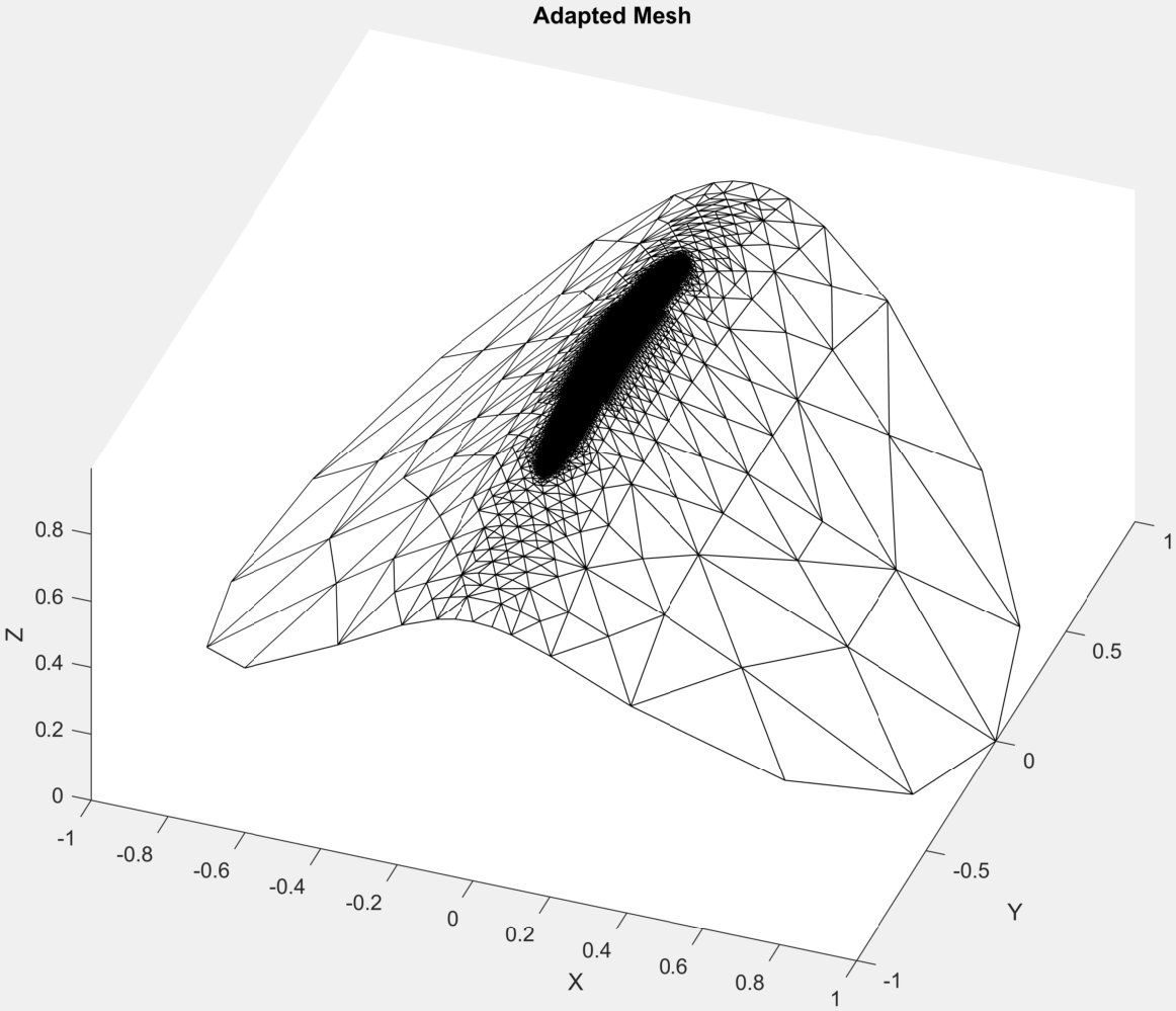 Figure 1
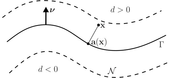 Figure 2
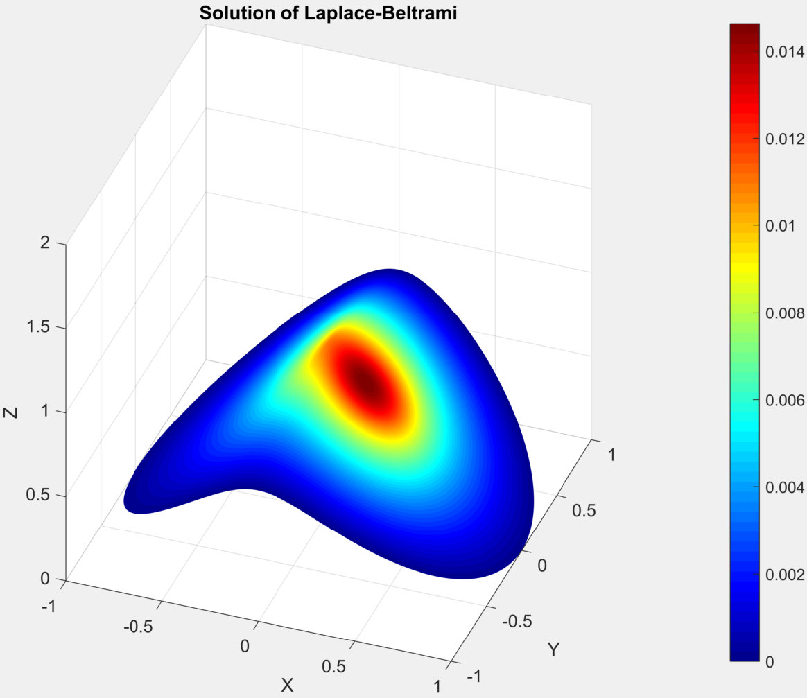 Figure 3
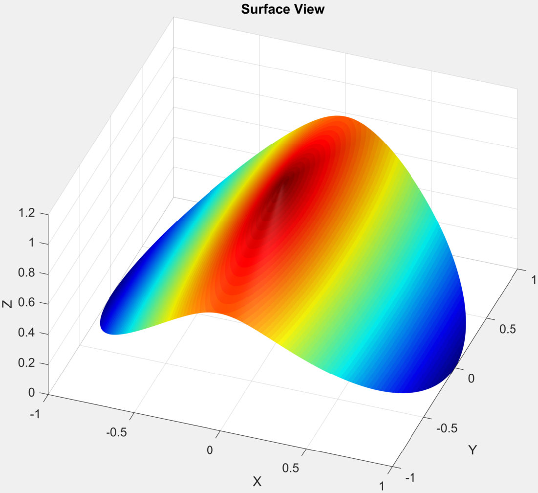 Figure 4
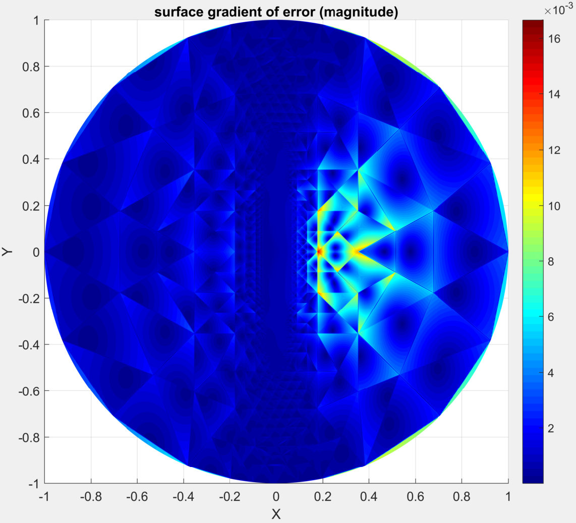 Figure 5
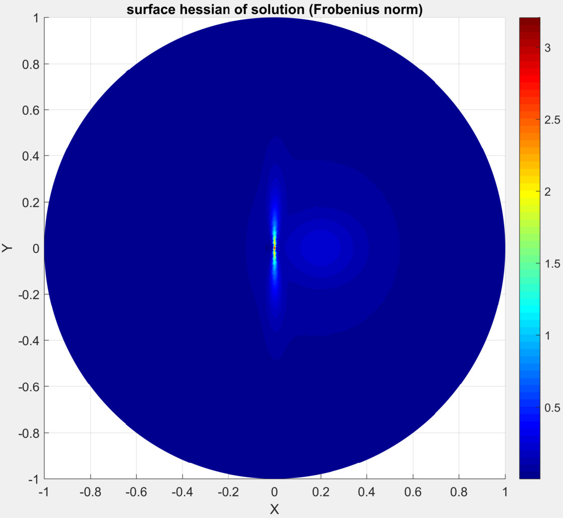 Figure 6
Peer Reviews
No public reviews on file for this paper yet. If you reviewed it on a platform where reviews are public (OpenReview, ICLR, NeurIPS, ICML), you can paste yours below so the community can read it here.
Videos
No videos yet. Explain this paper in a talk, walkthrough, or lecture? Add one.
Analysis of the finite element method for the Laplace–Beltrami equation on surfaces with regions of high curvature using graded meshes
Johnny Guzman, Alexandre Madureira, Marcus Sarkis and Shawn Walker
(Date: May 10, 2016)
Abstract.
We derive error estimates for the piecewise linear finite element approximation of the Laplace–Beltrami operator on a bounded, orientable, , surface without boundary on general shape regular meshes. As an application, we consider a problem where the domain is split into two regions: one which has relatively high curvature and one that has low curvature. Using a graded mesh we prove error estimates that do not depend on the curvature on the high curvature region. Numerical experiments are provided.
1. Introduction
Since the publication of the seminal paper [MR976234], there has been a growing interest in the discretization of surface partial differential equations (PDEs) using finite element methods (FEMs). Such interest is motivated by important applications related to physical and biological phenomena, and also by the potential use of numerical methods to answer theoretical questions in geometry [MR976234, MR3038698, MR3486164].
In this paper, we focus on linear finite element methods for the Poisson problem with the Laplace–Beltrami operator on , a two-dimensional compact orientable surface without boundary. That is, we consider
[TABLE]
In order to motivate the results in our paper, we start by giving a short overview of previous results. A piecewise linear finite element method is proposed and analyzed in [MR976234, MR3038698]. The basic idea is to consider a piecewise linear approximation of the surface, and pose a finite element method over the discretized surface. Discretizing the surface, of course, creates a geometric error, however, the advantage is that for a given discretization a surface parametrization is not necessary.
In [MR2485433] a generalization of the piecewise linear FEM is considered, based on higher order polynomials that approximate both the geometry and the PDE; the same paper proposes a variant of the method which employs parametric elements, and the method is posed on the surface, originating thus no geometric error. Discontinuous Galerkin schemes are considered in [MR3338674, MR3081490], and HDG and mixed versions are considered in [MR3522964]. Adaptive schemes are presented in [Bonito, MR3447136, MR2285862, MR2970758]. An alternative approach, where a discretization of an outer domain induces the finite element spaces is proposed in [MR2551197, MR2570076]. See also [MR3312662, MR3345245, MR2970758, MR3215065, MR3194806]. In [MR1868103, MR2608464, MR3043557, MR3471100], the PDE itself is extended to a neighborhood of the surface before discretization.
Other problems and methods were considered as well, as a multiscale FEM for PDEs posed on rough surface [MR3053884], and stabilized methods [MR3312662, hanslar, MR3371354, MR3194806]. In [MR2915563] the finite element exterior calculus framework was considered. Finally, transient and nonlinear PDEs were also subject of consideration, as reviewed in [MR3038698].
A common ground between all aforementioned papers is that the a-priori choices of the surface discretization do not consider how to locally refine the mesh following some optimality criterion. It is however reasonable to expect that some geometrical traits, as the curvatures, have a local influence on the solution, and thus the mesh refinement could account for that locally. Not surprisingly, numerical tests using adaptive schemes confirm that high curvature regions require refined meshes [MR3447136, Bonito]. This is no different from problems in nonconvex flat domains, where corner singularities arise, and meshes are used to tame the singularity at an optimal cost [MR0502065, MR0502067].
As far as we can tell, the development and analysis of a-priori strategies to deal with high curvature regions have not been an object of investigation, so far. In this paper we consider a simple setting: We suppose that the domain , and assume that the maximum of the principal curvatures in is much larger than those in . We then seek a graded mesh that gives us optimal error estimate. Of course, in the region the triangles will be much smaller than the mesh size in regions far from . We consider the method originally proposed by Dziuk [MR976234].
To carry out the analysis, we first need to track the geometric constants carefully. This, as far as we can tell, has not explicitly appeared in literature, although it is not a difficult task. We do this by following [MR976234, MR3038698] although in some cases we give different arguments while trying to be as precise as possible. The estimate we obtain is found below in (39). If is the finite element solution approximation to then the result reads (see sections below for precise notation):
[TABLE]
Here is an approximation to , is the Poincaré’s constant, and the numbers , are geometric quantities. For instance, where is the diameter of the triangle and measures the maximum principal curvatures on ( is the surface triangle corresponding to ; see sections below). The important point here is that can be controlled locally. That is, if one wants to reach a certain tolerance, one needs to make small enough only depending on the geometry in .
On the other hand, does not depend only on the local geometry. In order to deal with this term, in the case of two sub-regions, we prove local regularity results. Combining the local regularity and the a-priori error estimate (39) we are able to define a mesh grading strategy and prove Theorem 14. The error estimate contained in Theorem 14 is independent of the curvature in region , and in some sense is the best error estimate one can hope for given the available information.
The paper is organized as follows. In Section 2 we set the notation and derive several fundamental estimates highlighting the influence of the curvatures. Section 3 regards the finite element and interpolation approximations. Finally, we present in Section 4 a local estimate and a mesh grading scheme culminating in an error estimate that is independent of the “bad” curvature. The paper ends with numerical results in Section 5.
2. Preliminaries
As mentioned above, we assume that is bounded, orientable, surface without boundary. Furthermore, we assume that there is a high curvature region , and define . For with , let be such that
[TABLE]
where . We denote by the tangential gradient [MR3486164], and (1) is nothing but the weak formulation of the Poisson problem for the Laplace–Beltrami operator. Existence and uniqueness of solution follows easily from the Poincaré’s inequality (Lemma 6) and the Lax–Milgram theorem. Details on the definition of are given below. Consider now a triangulation of the surface . By that we mean that is a two-dimensional compact orientable polyhedral surface, and denoting by the set of closed nonempty triangles such that , we assume that all vertices belong to , and that any two triangles have as intersection either the empty set, a vertex or an edge. Let and . For all assume that there is a three-dimensional neighborhood of where for every there is a unique closest point (see Figure 1) such that
[TABLE]
is the signed distance function from to and is the unit normal to at , that is, ; with an abuse of notation, we define for . Note that by using local tubular neighborhoods, we avoid unnecessary restrictions on the mesh size.
Here we would like to explain some notational conventions that we use. From now on, the gradient of a scalar function will be a row vector. The normal vector is a column vector (as well as which is defined below).
We can now define, for every , the surface triangle . Then . Let be the self-adjoint operator corresponding to the derivative of the Gauss map [MR0394451]. Since , then . And again we set for .
At the estimates that follow in this paper we denote by a generic constant that might not assume the same value at all occurrences, but that does not depend on , , or on . It might however depend for instance on the shape regularity of .
Given , let
[TABLE]
and be unit-normal vector to such that . We note that since is symmetric, is also equivalent to the norm of the spectral radius of , or where the are the principal curvatures.
Assumption: Throughout the paper we will assume
[TABLE]
where is sufficiently small.
It is easy to see that
[TABLE]
To show (5), assume without loss of generality that and that , . Let be the Lagrange linear interpolant of in . Since vanishes at the vertices, . By [MR2050138] we have
[TABLE]
for . Next, to prove (6), start by noting that , and then the estimate for the first two components of follow from (7) and (3). The third component estimate follows from
[TABLE]
Here we used (4).
[TABLE]
Therefore, making sufficiently small in (4) so that the eigenvalues of are smaller or equal to for every , then we will have
[TABLE]
We define tangential projections onto and , respectively, as and , where for two column vectors and . We recall that the tangential derivatives for a functions defined on a neighborhood of (or ) are given by
[TABLE]
By using that , we have
[TABLE]
Hence, we, of course, have
[TABLE]
which we use repeatedly. Also, we can show that
[TABLE]
Indeed, by (11) and so .
2.1. Local parametrization
Let be the reference triangle. Fix , let be one of the vertices, and let and be vectors in representing two edges of (i.e. ). Let be given by . We also define by . Since we have . From the definition of we have
[TABLE]
and, hence
[TABLE]
Therefore, using that and are symmetric and (11) we have . Collecting the two results we have
[TABLE]
Given a function we define the pullback lift as
[TABLE]
and for we define the push-forward lift as
[TABLE]
and associate defined by
[TABLE]
Note that for and for .
Consider also the metric tensors
[TABLE]
From the definition of tangential derivative it is possible to show [MR3486164]*Section 4.2.1 (see also (2.2) in [MR3038698]) that for a function ,
[TABLE]
and multiplying by and we gather that
[TABLE]
Hence,
[TABLE]
Note that we can also write
[TABLE]
To see that this is the case, note first from (15) that . Next, consider for an arbitrary differentiable curve and . Then
[TABLE]
since is tangent to . The same arguments hold for the identity regarding .
The following identities have appeared in the literature under different forms; see for example [MR2485433, MR2285862]. Again, we give a proof for completeness and to show the independence of with respect to .
Lemma 1**.**
Let be differentiable, and define its forward lift as in (16). It then holds that
[TABLE]
where , and
[TABLE]
where R=\bigl{[}I-\frac{({\boldsymbol{\nu}}_{h}-{\boldsymbol{\nu}})\otimes({\boldsymbol{\nu}}-{\boldsymbol{\nu}}_{h})}{{\boldsymbol{\nu}}_{h}\cdot{\boldsymbol{\nu}}}\bigr{]}(I-dH)^{-1}P. Moreover, there exists a constant such that
[TABLE]
Proof.
[TABLE]
where we used that . Then (21) follows from (20).
To prove (22), we use (14) and (12) to get . Hence, we have
[TABLE]
Using (12) we get
[TABLE]
However,
[TABLE]
This gives
[TABLE]
So, from (25), (24) and (15) we have
[TABLE]
Thus, using (19) and the above identity we gather that
[TABLE]
from (20). Clearly we have , and follows from (13). So we get
[TABLE]
Here we used that . This proves (22). Finally, (23) follows from (6), (8), (9) and (4). ∎
Next, we write an integration identity.
Lemma 2**.**
Let . Then, if is the surface measure in and is the surface measure in it follows that
[TABLE]
where
[TABLE]
Proof.
The result follows from the change of variables formulas [MR0394451]
[TABLE]
∎
Combining (26), (21) and (22), we have that
[TABLE]
Next, we prove some bounds for .
Lemma 3**.**
Assuming that (4) holds and defining by (27) we have that
[TABLE]
Proof.
[TABLE]
Using (11) we get
[TABLE]
By (15),
[TABLE]
Hence,
[TABLE]
Therefore, we get
[TABLE]
or where . Therefore,
[TABLE]
It is clear that . Also, not difficult to see that . Moreover, using (6) and (8) we gather that . Hence, . Since is symmetric, consider the spectral decomposition , where and is orthogonal. Denoting the ith column of by , we have that and then (for ). We also note that
[TABLE]
Therefore, we obtain
[TABLE]
which yields
[TABLE]
Using that , we obtain (30). The inequality (31) follows from the previous inequality and the fact . ∎
We can now state the following result which follows from Lemmas 1 and 3, and equations (28), (29).
Lemma 4**.**
Assuming the hypotheses of Lemmas 1 and 3, we have that
[TABLE]
In the following, we use the notation , and write as the matrix with entries (also denoted by ).
Lemma 5**.**
Assuming that (4) holds, we have
[TABLE]
where .
Proof.
Let . Using (21) we see that for ,
[TABLE]
where we use Einstein summation convention.
Using the product rule and the fact that is constant we have
[TABLE]
where
[TABLE]
We start with . Using (21) we have
[TABLE]
Hence, using (23), (26), (30) and (4) we get
[TABLE]
If we combine this inequality with (8) and (4), we have
[TABLE]
Next, using (10) and the fact , we obtain
[TABLE]
Hence, using (6), (3), (26), (30) and (4) yields
[TABLE]
Similarly, (5), (26), (30) and (4) yield
[TABLE]
Combining the above estimates gives the desired result. ∎
3. Finite Element Spaces and local approximations
We introduce the following finite dimensional approximation of (1). The finite element space is given by
[TABLE]
For with , let such that
[TABLE]
Existence and uniqueness of the finite-dimensional problem (32) follows from noting that if is a solution with , then must be constant with zero average. Thus .
We will need a Poincaré’s inequality, as follows [MR3038698].
Lemma 6**.**
Assuming a two-dimensional compact orientable surface without boundary, there exists a constant such that
[TABLE]
Then we can state a simple energy estimate.
Lemma 7**.**
Let solve (1), then
[TABLE]
Before proving an a-priori estimate for we will need to prove an important lemma that measures the inconsistency in going from to . First, we need to develop notation to use in the next proof. Since with respect to a given triangle and its lifting , let us define
[TABLE]
Lemma 8**.**
Let and belong to . Then the following holds
[TABLE]
where .
Proof.
Using (26) we get
[TABLE]
Hence, (36) follows from (31).
To prove (35) we use (28) to get
[TABLE]
Using that we have
[TABLE]
where
[TABLE]
On the other hand, again using that we get
[TABLE]
Hence,
[TABLE]
We now proceed to bound . We first use (12), to get on
[TABLE]
Hence, we get
[TABLE]
where , and then the triangle inequality yields
[TABLE]
Now using (8), (4) and (31) and the fact that is bounded we obtain
[TABLE]
Since we have that on ,
[TABLE]
Finally using that we have
[TABLE]
Therefore, it follows from (6) that . Using the previous inequalities we obtain
[TABLE]
and hence
[TABLE]
and thus (35) follows from this inequality and (37). ∎
Theorem 9**.**
Let be the solution of (1) and let that solves (32). Assume that satisfies . Then there exists a constant such that
[TABLE]
where is as in Lemma 8.
Proof.
For an arbitrary , set and . By Lemma 4 we have
[TABLE]
Then, we write for an arbitrary constant
[TABLE]
where after using that ,
[TABLE]
By applying (36) and the Poincaré’s inequality (33) we get
[TABLE]
where we chose . Using the Cauchy-Schwarz inequality and the Poincaré’s inequality (33) we have
[TABLE]
Using the Cauchy-Schwarz inequality we get
[TABLE]
Using (35) gives
[TABLE]
Hence, combining the above results we get
[TABLE]
where we used that . If we use the triangle inequality and (34) we obtain
[TABLE]
The result now follows after taking the minimum over and use the fact that which follows from (4). ∎
Let be the standard Lagrange interpolant in onto and define . We then have the following estimate.
Lemma 10**.**
Let be the solution of (1). Then,
[TABLE]
where and was defined in Lemma 5.
Proof.
Recall that is the pullback lift of . Using Lemma 4, and approximation properties of the Lagrange interpolant, we have
[TABLE]
We get from Lemma 5 that
[TABLE]
The result follows easily by summing over and applying (34). ∎
We can combine Theorem 9 and Lemma 10 to get the following theorem.
Theorem 11**.**
Assume that the hypothesis of Theorem 9 holds. Then,
[TABLE]
4. Graded meshes for two subdomains
In this section we consider the case where there is a high curvature region , and . We let and assume that . We also let . We use our above results from the previous sections and local regularity results in order to grade a mesh so that the error is balanced.
We start by just stating the global regularity result which is found in [MR3038698]. We note that this result does not fit our graded meshing strategy; instead, we establish Lemma 13.
Lemma 12**.**
Assume that is a orientable compact surface without boundary, and that solves (1). Then , and there exists a constant that is independent of the curvatures of such that
[TABLE]
Applying Theorem 11 and Lemma 12 it easily follows that
[TABLE]
Then, requiring we get
[TABLE]
Of course, this is not a very good estimate in the case since we would have the mesh size far away from still depending on . Instead, we would like to have the mesh size to only depend on a distant order one away from . In order to do this we will need a local regularity result, as follows.
Lemma 13** (Weighted- regularity).**
Let be the solution of (1), and consider the subset . Let be such that . Then there is an universal constant such that
[TABLE]
Proof.
Note that , and
[TABLE]
Then
[TABLE]
From Lemma 17,
[TABLE]
Thus,
[TABLE]
The result now follows after using the energy estimate (34). ∎
Lemma 13 holds with a generic function , but we will apply the result with which is a 1-Lipschitz function.
4.1. The graded mesh
We start by defining d_{1}=\bigl{(}1+c_{p}(1+\kappa^{(2)})\bigr{)}/(1+c_{p}\kappa^{(1)}). We then define the region . We also let and define . We set . Finally, we let and also set for all , where is defined using the geodesic distance [MR1941909] and .
Our graded mesh will then satisfy: {labeling}M3
for every
for every
We recall that and were respectively defined in Theorem 9 and Lemma 10.
A few comments are in order. First, note that condition (M1) is completely local, and in the case , condition (M1) would be necessary to get an estimate of the form (41), as the argument above (41) shows.
Note that if then . The mesh size for triangles that are unit distance from (i.e. ) can be chosen so that . In the intermediate region a grading giving by (M3) needs to be satisfied. Finally, note that there is a smooth transition for triangles in the border of . Indeed, if then by (M3),
We now state and prove our main result.
Theorem 14**.**
*Suppose that solves (1) and solves (32). Assume that the mesh satisfies *(M1-M3). Then we have
[TABLE]
Before proving the result let us state a few comments. Note that the right hand side of (43) looks like the right hand side of (41) with instead of . Therefore, with the available information, (43) is essentially the best result we can hope for. So, we found a graded mesh where one has a fine mesh in the region where the curvature is high to get the best error estimate.
Proof.
(of Theorem 14) By (39) and our assumption (M1) we have
[TABLE]
Next, we estimate
[TABLE]
By our (M2) we get
[TABLE]
and we gather from Lemma 12 that
[TABLE]
The other term we bound in the following way by using (M3):
[TABLE]
Now using (42), we have
[TABLE]
The result now follows. ∎
4.2. An estimate
We now derive an error estimate in the norm, based on the usual duality argument. We note that the conditions (M1-M3) are no longer enough to guarantee a convergence that is independent of . Actually, (M1) is reinforced by imposing that {labeling}M3
Theorem 15**.**
*Suppose that solves (1) and solves (32). Assume that satisfies , and that the mesh satisfies *(M1-M4). Then we have
[TABLE]
Here .
Proof.
First, let be the weak solution of
[TABLE]
where
[TABLE]
Then
[TABLE]
where we used (1). Then, using (32), the fact that derivatives of constants are zero, and that , we can show that
[TABLE]
where
[TABLE]
Here we choose . Using (36), the Poincaré’s inequality (33), and that ,
[TABLE]
Using the Poincaré’s inequality (33) we get
[TABLE]
Using (35) we get
[TABLE]
Using the triangle inequality and the energy estimate (34) we have
[TABLE]
To bound we use the Cauchy-Schwarz inequality
[TABLE]
Using Lemma 10 we get the estimate
[TABLE]
As we did in the proof of Theorem 14 (using (M1-M3)) we can show that
[TABLE]
Hence, using (M1) we have
[TABLE]
Therefore, we get the bound
[TABLE]
Using (44), the triangle inequality and a energy estimate we have
[TABLE]
It follows then that
[TABLE]
Therefore,
[TABLE]
We gather from (M4) and (43) that
[TABLE]
The triangle inequality yields
[TABLE]
We now use that and (36) to get
[TABLE]
Using the triangle inequality, (33) and (34) we gather that
[TABLE]
Finally, from (46), (4), and (M4) we have
[TABLE]
The result follows from this inequality and (45). ∎
Remark 16**.**
Although we only proved results for domains without boundaries, we anticipate that our analysis will carry over to surfaces with boundary. In fact, in the next section we will provide numerical experiments for a surface with a boundary.
5. Numerical Experiments
We consider a simple example of a surface with a high curvature “ridge,” and show our adapted mesh as well as properties of the solution.
5.1. Surface Parameterization
Let be the surface parameterized by
[TABLE]
where (see Figure 2). The curvature regions , are defined by
[TABLE]
This leads to the following maximum curvatures on , :
[TABLE]
5.2. “Exact” Solution
We use zero boundary conditions on and choose the right-hand-side to be
[TABLE]
Note that is similar to a “bump” function [MR1476913] and is and has compact support on .
In lieu of an exact analytic solution, we compute a reference “exact” solution (denoted ) on a mesh consisting of 3,679,489 vertices and 7,356,928 triangles obtained from refining an initial coarse mesh. The number of free degrees-of-freedom of the reference solution is 3,677,441 (after eliminating boundary degrees-of-freedom). See Figure 3 for a plot of .
We also plot an approximation of to illustrate how the hessian is influenced by the high curvature of the domain, which is concentrated at the high curvature ridge of the surface (see Figure 4).
5.3. Adapted Mesh And Solution
Our adapted mesh is generated by first starting with a coarse mesh that satisfies (8), (4), (9). We then iteratively check the criteria in (M1), (M2), (M3) in Section 4.1. At each iteration, if any triangle does not satisfy the criteria, then it is marked for refinement. We then refine all marked triangles using standard longest-edge bisection. Figure 5 shows a plot of our final adapted mesh.
Figure 6 shows the “pointwise” error , where is the numerical solution on the adapted mesh. Note that the graded mesh, essentially, eliminates the error in the high curvature region. However, the grading strategy does not specifically account for , so the error is larger where is large.
Appendix A One technical result
Lemma 17**.**
Assume that is a two-dimensional compact orientable surface without boundary, and that . Then
[TABLE]
Proof.
In what follows, we use the two identities [MR3038698]
[TABLE]
and
[TABLE]
for all functions , . Also we will use that of course
[TABLE]
We assume for the proof that , and the general result follows from density arguments. Following [MR3038698]*Lemma 3.2, and using the Einstein summation convention,
[TABLE]
To handle the first term on the right hand side, we use (51) and the fact that to write:
[TABLE]
where we used (52) in the last equation. But , and then
[TABLE]
In the last equation we used (50) and (52). This completes the proof. ∎
References