
TL;DR
This paper investigates the properties of a prime product defined via base-$p$ digit sums, linking it to Bernoulli polynomials and exploring its prime divisor structure with conjectures on its asymptotic behavior.
Contribution
It establishes a connection between the prime product and Bernoulli polynomial denominators, and formulates a conjecture on the asymptotic number of large prime divisors.
Findings
(n) equals the denominator of Bernoulli polynomial difference
_n^+ has fewer than (n) prime divisors
Conjecture: _n^+ ext{ has about } rac{ ext{ (n)}}{ ext{log } n} \text{prime divisors asymptotically}
Abstract
We study the properties of the product, which runs over the primes, where denotes the sum of the base- digits of . One important property is the fact that equals the denominator of the Bernoulli polynomial , where we provide a short -adic proof. Moreover, we consider the decomposition , where contains only those primes . Let denote the number of prime divisors. We show that , while we raise the explicit conjecture that with a certain constant , supported by several computations.
Click any figure to enlarge with its caption.
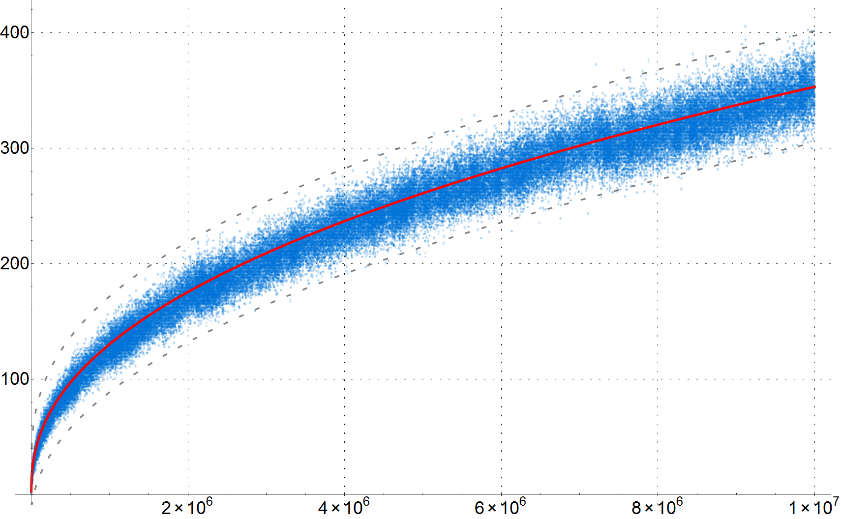 Figure 1
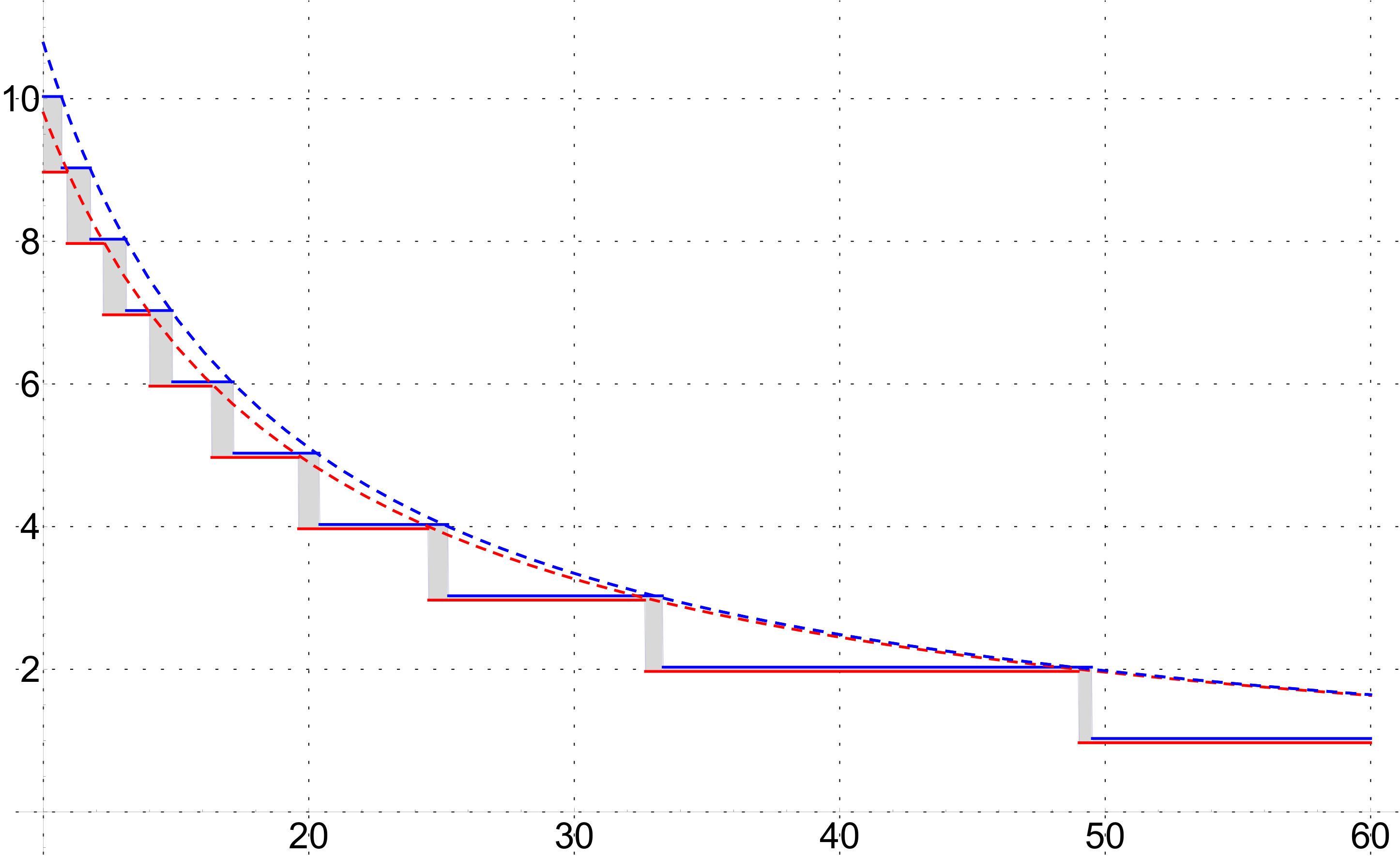 Figure 2
Peer Reviews
No public reviews on file for this paper yet. If you reviewed it on a platform where reviews are public (OpenReview, ICLR, NeurIPS, ICML), you can paste yours below so the community can read it here.
Videos
No videos yet. Explain this paper in a talk, walkthrough, or lecture? Add one.
On a product of certain primes
Bernd C. Kellner
Göttingen, Germany
Abstract.
We study the properties of the product, which runs over the primes,
[TABLE]
where denotes the sum of the base- digits of . One important property is the fact that equals the denominator of the Bernoulli polynomial , where we provide a short -adic proof. Moreover, we consider the decomposition , where contains only those primes . Let denote the number of prime divisors. We show that , while we raise the explicit conjecture that
[TABLE]
with a certain constant , supported by several computations.
Key words and phrases:
Product of primes, Bernoulli polynomials, denominator, sum of base- digits, -adic valuation of polynomials
2010 Mathematics Subject Classification:
11B83 (Primary), 11B68 (Secondary)
1. Introduction
Let be the set of primes. Throughout this paper, denotes a prime, and denotes a nonnegative integer. The function gives the sum of the base- digits of . Let denote the greatest prime factor of , otherwise . An empty product is defined to be .
We study the product of certain primes,
[TABLE]
which is restricted by the condition on each prime factor . Since in case , the product (1) is always finite.
The values are of basic interest, as we will see in Section 2, since they are intimately connected with the denominators of the Bernoulli polynomials and related polynomials.
Theorem 2 below supplies sharper bounds on the prime factors of . For the next theorem, giving properties of divisibility, we need to define the squarefree kernel of an integer as follows:
[TABLE]
Theorem 1**.**
The sequence obeys the following divisibility properties:
- (a)
Any prime occurs infinitely often:
[TABLE] 2. (b)
Arbitrarily large intervals of consecutive members exist such that
[TABLE] 3. (c)
Arbitrarily many prime factors occur, in particular:
[TABLE]
Theorem 2** (Kellner and Sondow [3]).**
If , then
[TABLE]
where
[TABLE]
In particular, the divisor is best possible, respectively the bound is sharp, for odd and even , when is an odd prime.
The divisor can be improved by accepting additional conditions.
Theorem 3**.**
The divisor holds in Theorem 2,
- (a)
if , 2. (b)
if is even and , 3. (c)
if is odd and .
The optimal divisor , which could replace in Theorem 2, obviously satisfies
[TABLE]
First values of , , and are given in Table A1. Supported by some computations, we raise the following conjecture, which implies an upper bound on .
Conjecture 1**.**
We have the estimates that
[TABLE]
We further introduce the decomposition
[TABLE]
where
[TABLE]
Note that the omitted condition has no effect on the above decomposition. Indeed, if , then and so . We keep in mind that the prime factors of are implicitly bounded by Theorem 2. Let \mathopen{}\mathclose{{}\left[\,\cdot\,}\right] denote the integer part. Define the additive function counting the prime divisors of .
Theorem 4**.**
If , then
[TABLE]
Moreover, we have the estimates
[TABLE]
The estimate of is apparently better than counting primes in the interval \bigl{[}\sqrt{n},\frac{n+1}{\lambda_{n}}\bigr{]} by the prime-counting function , while the obvious estimate is sharp, see Table A2.
Conjecture 1 is equivalent to for . On the basis of advanced computations, we raise the following conjecture, which gives even more evidence to hold with a better approximation.
Conjecture 2**.**
There exists a constant such that
[TABLE]
Computations up to suggest the value in that range and an error term , see Figure B1. Conjecture 2 implies at once the much weaker Conjecture 1 for sufficiently large values. However, both conjectures remain open.
Note that Theorem 2, as well as Theorem 5 in the next section, were recently given by Sondow and the author in [3, Thm. 1, 2, 4] using other notations. We will choose here a quite different approach, starting from the more general product (1), to attain to Theorems 2 and 5 by means of -adic methods, which result in short and essentially different proofs.
Outline for the rest of the paper: The next section shows the relations between and the denominators of the Bernoulli polynomials in Theorem 5. Section 3 demonstrates the divisibility properties of and contains the proofs of Theorems 1 – 3. In Section 4 we use step functions on a hyperbola to give a proof of Theorem 4. Section 5 discusses the -adic valuation of polynomials and includes the proof of Theorem 5.
2. Bernoulli polynomials
The Bernoulli polynomials are defined by the generating function
[TABLE]
and are explicitly given by
[TABLE]
where is the th Bernoulli number. First values are
[TABLE]
while for odd , see [4, Chap. 3.5, pp. 112–125]. The von Staudt–Clausen theorem describes the denominator of the Bernoulli number with even index. Together with (3), we have the squarefree denominators
[TABLE]
In addition, we define the related polynomials
[TABLE]
which have no constant term. Considering the power-sum function
[TABLE]
it is well known that
[TABLE]
implying that is an integer-valued function. The denominators of the polynomials , , and are surprisingly connected with the product (1) as follows.
Theorem 5** (Kellner and Sondow [3]).**
If , then we have the relations
[TABLE]
For an explicit product formula of , we refer to [3, Thm. 4].
3. Divisibility properties
An integer has a unique finite -adic expansion with a definite and base- digits satisfying . The sum of these digits defines the function . Note that
[TABLE]
since if , and if . Moreover, we have some complementary results as follows.
Lemma 1**.**
If and is a prime, then
[TABLE]
Proof.
By assumption we have . Thus, we can write with . This implies . ∎
Lemma 2**.**
If is even and is a prime, then
[TABLE]
Proof.
Since is even, we infer that . If , then we only have the case , so . For odd we obtain with . Consequently, . ∎
Lemma 3**.**
Let , be an odd prime, and . Write . Then
[TABLE]
Proof.
The left inequation above yields
[TABLE]
Since and , we have , implying that . ∎
Proof of Theorem 1.
Let and be a prime. Recall the product of in (1).
(a) If and , then we can write
[TABLE]
with some . This implies and so . Since this holds for all , the prime occurs infinitely often as a divisor in the sequence .
(b) If , then . Let . For all with , one observes that
[TABLE]
yields no carries in its -adic expansion. Thus, we have . Since , the interval can be arbitrarily large.
(c) Neglecting the trivial case, we assume that is composite and so . For all prime divisors of we then infer by part (a) that . This shows that
[TABLE]
Now we construct for different primes an index such that
[TABLE]
implying that arbitrarily many prime factors can occur. ∎
Proof of Theorem 2.
By Lemma 1 and (7) we deduce for that
[TABLE]
holds with . If , then is odd and , showing that the bound is sharp in this case. Now, let be even. Since , we infer by using Lemma 2 as a complement that (8) also holds with . This defines for even , while for odd . If , then is even and , giving a sharp bound for that case. ∎
Proof of Theorem 3.
We have to determine the cases of , where holds in Theorem 2, or rather holds in (8). The exceptional cases and for odd are already handled by Theorem 2 providing the optimal values and , respectively.
Regarding entries of () in Table A1, one observes that only holds for in this range. This proves part (a).
Let . Since for (see Table A1), and for , the primes and are always considered in (8), when possibly taking . From now let be fixed. Write . We distinguish between the following two cases.
Case even: We have by Theorem 2. If , we infer by Lemma 3 with , that must hold. Since is even, the only exception can appear by parity if , so and . This defines the set of exceptions in this case.
Case odd: We have by Theorem 2. If , then we deduce from Lemma 3 with , that must hold. Since is odd and due to parity, the only exception can happen, when , so and . If also , then we derive from Lemma 3 with , that must hold. Again, the only exception can occur with , so and . This defines the set of exceptions in that case.
Consequently, if is even and , respectively is odd and , for all , then . This proves parts (b) and (c), completing the proof. ∎
4. Step functions
As usual, we write x=\mathopen{}\mathclose{{}\left[x}\right]+\mathopen{}\mathclose{{}\left\{x}\right\}, where 0\leq\mathopen{}\mathclose{{}\left\{x}\right\}<1 denotes the fractional part. We define for the step functions, giving the integer part of a hyperbola, by
[TABLE]
and their difference
[TABLE]
on the intervals . Note that
[TABLE]
Since we are here interested in summing the function , it should be noted that there is a connection with Dirichlet’s divisor problem. This can be stated with Voronoi’s error term as
[TABLE]
where is Euler’s constant. The exponent in the error term was gradually improved by several authors, currently to by Huxley, see [2, Chap. 10.2, p. 182]. Rather than using analytic theory, we will use a counting argument below. Before proving Theorem 4, we need some lemmas.
Lemma 4**.**
If , then
[TABLE]
Proof.
Let be fixed. By (12) it remains to consider the range . By using \mathopen{}\mathclose{{}\left[x}\right]=x-\mathopen{}\mathclose{{}\left\{x}\right\}, we easily infer that
[TABLE]
because all summands of the right-hand side lie in the interval . ∎
Lemma 5**.**
If and where , then
[TABLE]
Proof.
If , we must have , and we are done by (11) and (12). So it remains the case and . By (11) we conclude that for all . Since for by Lemma 4, it also follows that , and so , for all . Together with (12) this gives the result. ∎
Lemma 6**.**
If and is a prime, then
[TABLE]
Proof.
Let be fixed. If , then we have and by (7) and (12), respectively, and we are done. It remains the range . In view of Lemma 4, we have to show that
[TABLE]
for the prime in that range. Thus, we can write
[TABLE]
where a_{1}=\mathopen{}\mathclose{{}\left[\dfrac{n}{p}}\right]\geq 1. Substituting the -adic digits leads to
[TABLE]
If , then we deduce the following steps:
[TABLE]
Since the statements above also hold in reverse order, (13) follows. ∎
Lemma 7**.**
If , then
[TABLE]
Proof.
Let be fixed. Set \mathcal{I}_{n}:=\bigl{[}\mathopen{}\mathclose{{}\left[\sqrt{n}\,}\right]+1,n\bigr{]} and , where both sets are not empty. Considering Lemma 4 and (12), we have to count the events when for . The images and describe both a graded hyperbola (see Figure B2), being piecewise constant and divided into decreasing steps. From now on, we are interested in the properties of . For we call the height of the corresponding step in the interval .
Viewing the function on the interval , we observe the steps of decreasing heights
[TABLE]
where the heights are bounded by the values of on the boundary of , namely,
[TABLE]
Hence, we have a decomposition of into the disjoint intervals .
Now fix a height . Set . It turns out that on the interval the event can at most happen once. More precisely, must be the greatest possible integer (see gray areas in Figure B2). Assume to the contrary that there exist integers satisfying and . By definition we have . Thus, it also follows, since is constant on the interval , that , where . Putting all together, we then obtain that
[TABLE]
giving a contradiction.
As a consequence, we have now to count the intervals or rather the steps of different heights . In total, there are such ones by (14). Next we show that the step of height has to be excluded from counting. Indeed, this follows by Lemma 5, since for any with , we always have .
We finally deduce that
[TABLE]
It remains to show that . By (15) this turns into
[TABLE]
which holds by the stricter inequality
[TABLE]
implying the result. ∎
Proof of Theorem 4.
Let . First we show that
[TABLE]
By combining Lemmas 4, 6, and 7, we deduce that
[TABLE]
Rewriting the condition as in (13) finally yields (16).
Next we use the straightforward estimate
[TABLE]
By [6, Cor. 2, p. 69] we have
[TABLE]
with exceptions at \mathopen{}\mathclose{{}\left[x}\right]=113. More precisely, we have , while . Since , we infer that
[TABLE]
holds for all , finishing the proof. ∎
5. -adic valuation of polynomials
Let be the field of -adic numbers. Define as the -adic valuation of . The ultrametric absolute value is defined by on . Let be the usual norm on .
These definitions can be uniquely extended to a nonzero polynomial
[TABLE]
where . We explicitly omit the case for simplicity in the following. Define
[TABLE]
where gives the unsigned content of a polynomial, see [5, Chap. 5.2, p. 233] and [4, Chap. 2.1, p. 49]. The product formula then states that
[TABLE]
including the classical case as well. It also follows by definition that
[TABLE]
Before giving the proof of Theorem 5, we have two lemmas. To avoid ambiguity, e.g., between and , we explicitly write instead of below.
Lemma 8** (Carlitz [1]).**
If are integers and is a prime such that and , then
[TABLE]
Lemma 9**.**
If and is a prime, then
[TABLE]
Proof.
We initially compute by (2), (3), and (5).
Cases : We obtain and . Thus, we have , while , for all primes ; showing the result for these cases.
Now let . Since for odd , we deduce that
[TABLE]
Evaluating the coefficients of by (17), we show that
[TABLE]
On the one hand, is a monic polynomial implying that
[TABLE]
On the other hand, we derive that
[TABLE]
and for even with that
[TABLE]
since the von Staudt–Clausen theorem in (4) reads
[TABLE]
This all confirms (19). Next we consider the cases and separately.
Case : Since by (20), it remains to evaluate (21). Set . In view of (20) – (22), we use Lemma 8 to establish that
[TABLE]
Together with (19), this conversely implies that
[TABLE]
showing the result for .
Case , odd: We have by (20), and , since . Thus (23) holds for this case.
Case , even: Since by (20), we have to evaluate (21) and (22) once again. In order to apply Lemma 8 in the case with , we have to modify some arguments. Note that is even. Furthermore, if is even, so is , since
[TABLE]
Under the above assumptions we then infer that
[TABLE]
This finally implies (23) and the result in that case; completing the proof. ∎
Proof of Theorem 5.
Using the product formula (18), we derive from Lemma 9 that
[TABLE]
Hence, is a squarefree integer, giving the denominator, and by (1) we obtain
[TABLE]
Furthermore, we deduce from (4) and (5) that
[TABLE]
Finally, it follows by (6) that , and consequently that
[TABLE]
Conclusion
As a result of Lemma 9 and (24), the product (1) of is causally induced by the product formula and arises from the -adic valuation of . The bounds given in Theorem 2 are self-induced by properties of as shown by Lemmas 1 and 2.
Appendix A Tables
Table A1**.**
First values of are small, while subsequent values are volatile for larger indices ( rounded to decimal places):
[TABLE]
[TABLE]
Table A2**.**
Number of prime factors of compared to , where \pi_{n}:=\pi\bigl{(}\frac{n+1}{\lambda_{n}}\bigr{)} and \pi_{n}^{-}:=\pi\bigl{(}\sqrt{n}\bigr{)}:
[TABLE]
Appendix B Figures
To compute the graph of Figure B1 in a realizable time and due to the limited display resolution, successive values of up to were chosen by random step sizes in the range . Incorporating the different bounds according to odd and even arguments in Theorem 2, we computed both values of and for each chosen . To illustrate the frequency, the values were plotted by blue dots with an opacity of . All computations were performed by Mathematica.
Acknowledgment
The author is grateful for the valuable suggestions of the referee which improved the paper.
The reference list from the paper itself. Each links out to its DOI / PubMed record.
- 1[1] L. Carlitz, A divisibility property of the binomial coefficients , Amer. Math. Monthly 68 (1961), 560–561.
- 2[2] H. Cohen, Number Theory, Volume II: Analytic and Modern Tools , GTM 240 , Springer–Verlag, New York, 2007.
- 3[3] B. C. Kellner, J. Sondow, Power-Sum Denominators , Amer. Math. Monthly, to appear 2017/2018, Preprint ar Xiv: 1705.03857 [math.NT] .
- 4[4] V. V. Prasolov, Polynomials , 2nd edition, ACM 11 , Springer–Verlag, Berlin, 2010.
- 5[5] A. M. Robert, A Course in p 𝑝 p -adic Analysis , GTM 198 , Springer–Verlag, New York, 2000.
- 6[6] J. Rosser, L. Schoenfeld, Approximate formulas for some functions of prime numbers , Ill. J. Math. 6 (1962), 64–94.