Generation, dynamical buildup and detection of bi- and mulipartite entangled states in cavity systems
D. Pagel, H. Fehske

TL;DR
This paper explores methods to generate, enhance, and detect bipartite and multipartite entangled states in cavity quantum systems, including microcavities and driven emitter-cavity setups, highlighting new protocols and their robustness.
Contribution
It introduces novel schemes for entanglement generation in cavity systems, optimizing correlations, phase matching, and dynamical buildup, advancing quantum optical entanglement control.
Findings
Strong bipartite entanglement between polariton branches achieved.
Multipartite entanglement among cavity modes demonstrated.
Entanglement production is most effective during initial laser oscillations.
Abstract
We inspect different quantum optical setups from the viewpoint of entanglement generation and detection. As a first step we consider a planar semiconductor microcavity and optimize the Bell-type correlations and their robustness against dephasing to create strong bipartite entanglement between polariton branches, which subsequently can be transfered to the emitted photons. In a second step, in order to create multipartite entangled light, we place the microcavity in an optical resonator driven by pump pulses with a frequency comb spectrum. For this system we show how phase matching of all comb modes can be achieved and will lead to indistinguishable scattering processes causing entanglement among every mode. Finally we demonstrate the buildup of entanglement in the dissipative dynamics of emitters coupled to a single cavity photon mode driven by an external laser. From a Floquet master…
Click any figure to enlarge with its caption.
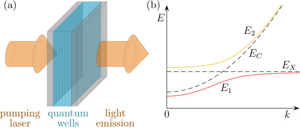 Figure 1
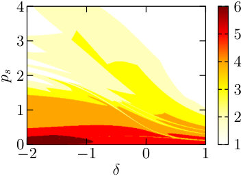 Figure 2
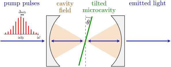 Figure 3
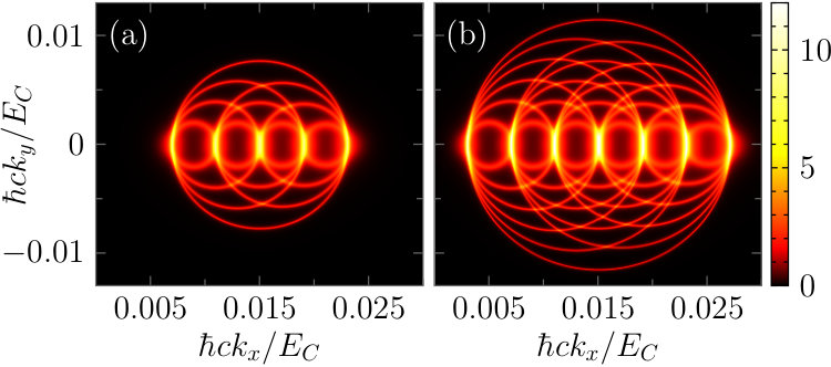 Figure 4
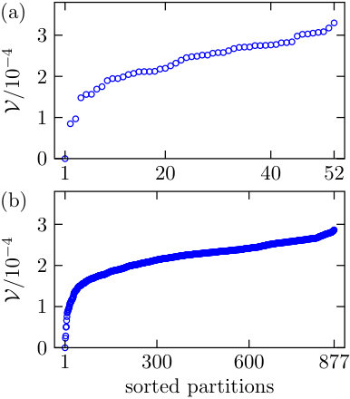 Figure 5
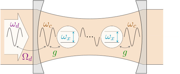 Figure 6
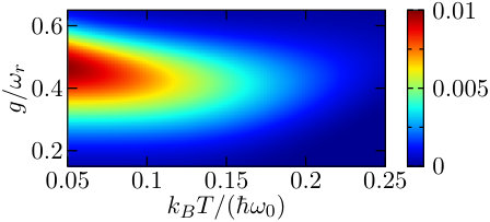 Figure 7
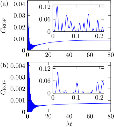 Figure 8
Peer Reviews
No public reviews on file for this paper yet. If you reviewed it on a platform where reviews are public (OpenReview, ICLR, NeurIPS, ICML), you can paste yours below so the community can read it here.
Videos
No videos yet. Explain this paper in a talk, walkthrough, or lecture? Add one.
Generation, dynamical buildup and detection of bi- and mulipartite entangled states in cavity systems
D. Pagel
H. Fehske
Institut für Physik, Ernst-Moritz-Arndt-Universität, 17487 Greifswald, Germany
Abstract
We inspect different quantum optical setups from the viewpoint of entanglement generation and detection. As a first step we consider a planar semiconductor microcavity and optimize the Bell-type correlations and their robustness against dephasing to create strong bipartite entanglement between polariton branches, which subsequently can be transfered to the emitted photons. In a second step, in order to create multipartite entangled light, we place the microcavity in an optical resonator driven by pump pulses with a frequency comb spectrum. For this system we show how phase matching of all comb modes can be achieved and will lead to indistinguishable scattering processes causing entanglement among every mode. Finally we demonstrate the buildup of entanglement in the dissipative dynamics of emitters coupled to a single cavity photon mode driven by an external laser. From a Floquet master equation approach we find that entanglement production predominates during the first few laser oscillation periods.
Quantum Optics, Open Systems, Entanglement Production
pacs:
03.65.Yz, 03.67.Bg, 42.50.-p,
I Introduction
Quantum entanglement Schrödinger (1935); Einstein et al. (1935); Horodecki et al. (2009); Nielsen and Chuang (2010), embodying a certain kind of correlation between subsystems without classical counterpart Werner (1989), is the fundamental resource for future quantum computation and communication applications Feynman (1982); Bennett and Wiesner (1992); Lloyd (1996). The most elementary realizations are Bell states in bipartite situations Bell (1964) and GHZ or W states Greenberger et al. (1989); Dür et al. (2000) in the event that more than two subsystems are entangled. In the multipartite case, a state is called partially entangled if some (but not all) subsystems can be separated, and fully entangled if subsystems can not be separated.
Theoretically, entanglement can be determined by so-called witnesses, exhibiting negative expectation values for entangled states Horodecki et al. (1996, 2001). A witness is an observable and thus can be measured in experiments. The problem is, that a positive expectation value does not allow to decide whether or not the state is entangled. To overcome this drawback an optimization was introduced Lewenstein et al. (2000), yielding necessary and sufficient conditions for the detection of entanglement Sperling and Vogel (2009, 2011a). In order to quantify the amount of entanglement of a given state, one has to construct a proper entanglement measure Vedral et al. (1997); Vidal (2000); Brandao (2005). Albeit this has been done for bipartite systems Brandao (2005); Sperling and Vogel (2011a, b), the general multipartite case resists a complete solution so far Sperling and Vogel (2013); Sperling and Walmsley (2017).
Also from an experimental point of view, despite recent progress Vandersypen et al. (2001); Cirac and Zoller (2004); de Valcárcel et al. (2006); Medeiros de Araújo et al. (2014), the generation and control of entangled states is a still challenging task, because the necessary quantum coherence usually rapidly decays. Entanglement distillation of non-maximally entangled states may be a route to overcome this problem Bennett et al. (1996, 1997); Horodecki et al. (1997). Alternatively, the experimental setup can be optimized to generate a high amount of entanglement. In this respect, optical realizations are promising DiGuglielmo et al. (2011). Entanglement generation then relies on strong interactions in hybrid light-matter systems. This regime is accessible in cavity-quantum or circuit-quantum electrodynamics setups Niemczyk et al. (2010); Agarwal (2013); Yoshihara et al. (2017) and is usually described by the famous Dicke model of two-level emitters coupled to a cavity photon mode Dicke (1954). Other approaches are based on parametric down-conversion in nonlinear crystals Kwiat et al. (1995); Axt and Kuhn (2004); Gerke et al. (2015), biexciton decay in quantum dots Benson et al. (2000); Hohenester et al. (2003), parametric interactions of cavity photons and semiconductor excitons in two-dimensional microcavities Weisbuch et al. (1992); Houdré et al. (1994); Langbein (2004); Ciuti et al. (2005), or nitrogen-vacancy centers in photonic crystals Yang et al. (2011); Wolters et al. (2014).
In this paper, we address the generation, evolution and detection of entanglement for three different quantum optical settings. First, we take up the idea that strong bipartite entanglement can be created by a two-dimensional semiconductor microcavity driven by a pump-pulse train Pagel et al. (2012). Tuning the system parameters, Bell-type correlations can be enforced, transferred to nonclassical light, and verified by the Schmidt decomposition of the system’s state. In this way, we identify the optimal parameter region for the generation of highly entangled light. Second, we propose a scenario where a planar microcavity is placed inside an optical resonator that is driven by lasers with a frequency comb spectrum. We show, that this system is capable of distributing entanglement among each mode of the comb leading to a highly multipartite entangled (continuous variable) state which again can be proved in the emitted light. Third, we demonstrate, analyze and quantify a dynamical buildup of (bipartite) entanglement among two emitters placed inside a laser-driven cavity. We find that the entanglement during the first few modulation periods is much higher than the asymptotic value at later times. This offers the possibility to enhance the entanglement by successive pump pulses.
The article is organized accordingly. Section II introduces the driven microcavity model and gives the Schmidt number at fixed dephasing in dependence on the detuning and the polariton splitting to binding energy ratio. Section III deals with multipartite entangled light starting from a frequency comb spectrum. Specifically, the phase-matching polariton interactions were studied in Sec. III.1, the ground state of the system is evaluated in Sec. III.2, and its entanglement properties are analyzed in Sec. III.3. Section IV describes the dynamics of entanglement between two emitters strongly coupled to a laser-driven cavity in terms of the Dicke model. Finally, Sec. V provides our conclusions.
II Planar semiconductor microcavity
We consider a planar semiconductor microcavity driven by external optical pumping [see Fig. 1(a)]. Such a system is usually described in terms of (bosonic) polaritons Usui (1960); Tassone and Yamamoto (1999); Ciuti et al. (2001, 2005), which provides an efficient framework to investigate polariton parametric scattering in momentum space Ciuti (2004); Langbein (2004). An alternative approach, which is based on the Heisenberg equations of motion for the semiconductor exciton and cavity photon operators, is the so-called dynamics controlled truncation formalism Axt and Stahl (1994); Savasta and Girlanda (1996a); Portolan et al. (2008a, b).
Polaritons are hybrid light-matter quasiparticles that arise from the strong coupling between semiconductor excitons and cavity photons Weisbuch et al. (1992); Houdré et al. (1994). During the process of polariton formation two branches emerge, whereby an avoided crossing of exciton and photon modes takes place [see Fig. 1(b)]. The energies of these polariton branches are
[TABLE]
where is the branch index, denotes the two-dimensional wave vector with modulus , is the cavity photon energy with , is the (dispersionless) exciton energy, and gives the vacuum Rabi splitting. The polariton dispersions in Fig. 1(b) show a clear asymmetry between the lower and upper branch which is a consequence of the normalized detuning as well as of the cavity and exciton energies.
Pumping with a laser resonantly injects polaritons with fixed wave vector and energy. The Coulomb interaction between the exciton constituents (electrons and holes) in combination with saturation effects in the course of bosonization of their actual fermionic excitations yields an effective polariton pair interaction Tassone and Yamamoto (1999); Östreich et al. (1998). Therefore, two pumped polaritons can scatter into pairs of signal and idler polaritons, if energy and momentum is conserved (phase-matching) Savvidis et al. (2000); Savasta et al. (2005); Portolan et al. (2009). One distinguishes single-pump from mixed-pump processes, where the two initial polaritons are injected by a single or two different pumped modes, respectively. The indistinguishability of the scattering channels for specific pump configurations is the key for the generation of entangled polaritons Ciuti (2004); Auer and Burkard (2012); Portolan et al. (2014); Einkemmer et al. (2015). Since the polaritons have a large photon component any polariton entanglement can efficiently be transfered to the emitted photons Weisbuch et al. (1992); Ciuti et al. (2001).
If a pump laser is split into multiple beams that are aligned on a cone with incident angle below the magic angle Langbein (2004); Savvidis et al. (2000), the generation of multipartite entangled W states becomes possible Pagel et al. (2013). This setup involves scattering within the lower polariton branch and seems therefore feasible in experiments Pagel and Fehske (2015). The multipartite correlations of the photons in the output channels can be identified with so-called multipartite entanglement witnesses which requires the solution of separability eigenvalue equations Sperling and Vogel (2013). Such a solution is given in Ref. Pagel et al. (2013) for a general witness constructed from W states allowing for the detection of light entanglement in the presence of lossy media.
Strong bipartite entangled states can be generated if the upper polariton branch is driven by a pump pulse train. Assuming a train of individual modes, the state of the corresponding branch-entangled polariton pairs takes the form Pagel et al. (2012)
[TABLE]
In this equation, is the polariton vacuum and creates a signal () or idler () polariton in the lower () or upper () branch. The index indicates that two pumped polaritons from mode of the train scatter into signal and idler, i. e., given a pump wave-vector we have and for a phase-matching scattering wave-vector . The constants characterize the properties of the material and explicitly read Pagel et al. (2012)
[TABLE]
Here,
[TABLE]
is an effective branch-dependent potential with the matrix elements of the Hopfield transformation Hopfield (1958)
[TABLE]
and the exciton binding energy .
The non-classical correlations of the emitted photons can be analyzed using the Schmidt number (SN) Terhal and Horodecki (2000); Sanpera et al. (2001); Sperling and Vogel (2011b), which quantifies the entanglement of a bipartite state based on the superposition of product states. For pure states the SN arises from the Schmidt decomposition of the state, that is, the SN counts the nonzero coefficients Nielsen and Chuang (2010). Hence, every separable state has a SN of 1. A maximally entangled Bell state has . is possible for subspace dimensions larger than one. A generalization to mixed quantum states can be achieved by a convex roof construction.
Here, we use SN witnesses Bruß et al. (2002); Sperling and Vogel (2011a); Pagel et al. (2012) to quantify the entanglement of the emitted photons that decreases due to propagation in dephasing channels, see Ref. Pagel et al. (2012) for details of this formalism. Our goal is to maximize the resulting SN in dependence on the normalized detuning and the ratio of polariton splitting to exciton binding energy to find the best system parameters for experimental implementation. In Fig. 2 the SN for with upper bound , given for a fixed dephasing time fs, is obtained by numerical optimization of the SN witness and thus gives a lower bound for the actual SN of the state. As a general trend, we find an increasing SN if the polariton splitting to binding energy ratio tends to zero. Moreover, a negative detuning makes the entanglement more robust against dephasing, at least if . This means that the initial state of the branch-entangled polariton pairs is given by a superposition of maximally entangled Bell states if and .
III Multipartite entanglement with frequency comb pulses
We now extend the system under consideration by placing the planar microcavity inside a cavity and tilting it by an angle from the vertical related to the incident light (see Fig. 3). The pump pulse itself represents a frequency comb with central frequency and line separation .
III.1 Polariton interaction
Defining an in-plane wave-vector and we find that pumping the microcavity with a frequency comb generates polaritons at the equidistant points in -space, where and is the number of (pump) spectral lines above and below the central frequency . Phase-matching scattering processes between all frequencies of the comb can be achieved when the lower polariton branch is pumped below the magic angle. The scattering channels in line with that are depicted in Fig. 4, which visualizes the phase-matching function
[TABLE]
In Eq. (6), denotes the polariton broadening.
In what follows, we consider the case for in Fig. 4(a) and in Fig. 4(b). We expect, that the pumped modes become entangled because the different mixed-pump scattering processes are indistinguishable. Then, the Hamiltonian describing the polaritons and their scattering processes takes the form
[TABLE]
where () creates (annihilates) a polariton in the lower branch with wave-vector . The coupling of the different modes is given by the (real) matrix elements
[TABLE]
Here, is the radius of the semiconductor exciton, is the sample surface, and is the pump spectral amplitude of mode .
III.2 Polariton ground state
The ground state of the Hamiltonian (7) is a Gaussian state. Introducing the amplitude and the phase quadrature of the individual modes, we define a vector of quadratures . Its expectation values
[TABLE]
are the entries of the Gaussian state’s covariance matrix \boldsymbol{\Sigma}=\big{\langle}\hat{\boldsymbol{\xi}}\hat{\boldsymbol{\xi}}^{T}\big{\rangle}-\big{\langle}\hat{\boldsymbol{\xi}}\big{\rangle}\big{\langle}\hat{\boldsymbol{\xi}}\big{\rangle}^{T}, where . To determine the covariance matrix, we rewrite the Hamiltonian (7) using quadrature operators,
[TABLE]
where the real symmetric () and positive definite () matrix has a block structure
[TABLE]
The ground state is given by the normalized, Gaussian wave-function
[TABLE]
where are the coordinates, and is also a real symmetric and positive definite matrix. Then the corresponding eigenvalue problem reads
[TABLE]
This equation is solved by the ground state if
[TABLE]
The corresponding ground-state energy is
[TABLE]
Finally, the covariance matrix follows from transformation to the Wigner representation:
[TABLE]
III.3 Multipartite entanglement between continuous variables
The complexity of entanglement is realized if a system consisting of a manifold of parties is considered. For example, a subsystem can be entangled with a second one but separated from a third one. However, the third subsystem may still be entangled with the second one. The number of such different forms of multipartite entanglement rapidly increases with the number of parties. Nevertheless, different techniques to tackle entanglement in such systems have emerged Adesso et al. (2004); Gerke et al. (2015); Sperling and Vogel (2013).
To determine the multipartite continuous-variable entanglement of the polariton ground state (12) we again use the witnessing method Sperling and Vogel (2013); Gerke et al. (2015). In particular, the Gaussian state with covariance matrix is entangled with respect to a partition if and only if a Hermitian operator with
[TABLE]
exists Horodecki et al. (1996, 2001). In Eq. (17), the modes are partitioned into different and complementary subsystems and is the minimum expectation value of among all separable states of this partition. Because the first-order moments are irrelevant for entanglement, without loss of generality, we may assume a state with
[TABLE]
Next, we need to find a particular Hermitian operator that fulfills Eq. (17). According to Ref. Sperling and Vogel (2013), the optimal choice is for the detection of entanglement within the ground state (12) of . Then, the left-hand side of condition (17) readily follows as
[TABLE]
and the right-hand side becomes Sperling and Vogel (2013); Gerke et al. (2015)
[TABLE]
Here, the submatrix of that contains only the rows and columns belonging to the index set is .
With Eqs. (17), (19), and (20) we have all ingredients for the detection of multipartite entanglement. To visualize the results we introduce the so-called entanglement visibility Sperling and Walmsley (2017)
[TABLE]
that quantifies the fulfillment of condition (17). takes positive (negative) values if the state is entangled (not entangled) with respect to the chosen partition. A large positive value of indicates a sufficient separation between the left-hand and right-hand sides of Eq. (17). The closer is to zero the higher is the required resolution of a corresponging detector that measures . Nevertheless, does not quantify multipartite entanglement. To the best of our knowledge, a single universal measure of multipartite entanglement does not exist so far.
In Fig. 5 we plot the visibility of each partition’s entanglement for and with a total of and modes, respectively. The so-called Bell number of possible partitions is determined from combinatorics. For example, the set of three modes has five partitions: 1:2:3, 12:3, 13:2, 1:23, and 123. Likewise, one obtains 52 (877) partitions for a set of five (seven) modes.
Since for each partition in Fig. 5, we can conclude that each subsystem is entangled with all the other subsystems. In Figs. 5(a) and 5(b), the points with correspond to the trivial partition , where all modes are incorporated in a single party only. This partition is necessarily not entangled. All other partitions have a positive entanglement visibility, such that the polariton ground state is proven to be fully multipartite entangled. In other words, entanglement will be distributed among each mode of the initial frequency comb pump pulse once the light interacts with the microcavity.
IV Dissipative buildup of entanglement in a Dicke-type cavity
The results presented so far do not take account of effects arising from dissipation, that is, from the coupling to environmental degrees of freedom. Therefore, in this section, we study the dissipative dynamics of entanglement in the strong light-matter coupling regime. In particular, we are interested in the entanglement between two two-level emitters (qubits) that are placed inside a cavity which itself is driven by an external laser, see Fig. 6. Such a situation can be described by the driven Dicke model Dicke (1954):
[TABLE]
In Eq. (22), () creates (annihilates) a cavity photon with frequency , () incorporates the relaxation (excitation) of the th emitter with transition energy . The emitter-cavity coupling strength is . The driving amplitude and frequency are denoted by and , respectively. In what follows we only consider the resonance situation: .
A consistent theoretical description of strongly interacting quantum optical systems coupled to the environment is difficult, even in the simplest case, when dissipation can be treated in the Markovian approximation (for previous approaches, see, e. g., Refs. Carmichael (1999); Breuer and Petruccione (2002); Weiss (2012); Agarwal (2013); Schaller (2014)). Starting from the Dicke model (22) without drive , it is necessary to replace the standard quantum optical master equation by a master equation expressed in the photon-dressed emitter states Beaudoin et al. (2011); Alicki et al. (2006); Schaller and Brandes (2008); Ridolfo et al. (2013). Combining this equation with the input-output formalism Collett and Gardiner (1984); Gardiner and Collett (1985); Graham (1989); Savasta and Girlanda (1996b), the statistics of the emitted photons can be evaluated, showing that cooperative effects lead to the generation of nonclassical light already at weak light-matter coupling if the number of emitters is increased Pagel et al. (2015). For finite driving the approach developed in Ref. Pagel et al. (2017) can be used to monitor the dynamics of the system, e.g., in order to analyze the dynamic Stark effect via the shifting of spectral lines in the emission spectrum.
Here, we consider a Dicke-type cavity coupled to bosonic environmental degrees of freedom with interaction Hamiltonian where is a Hermitian system operator and are annihilation operators of environment photons at frequencies with coupling constants . We choose for the interaction of the cavity and for the interaction of the th emitter with the environment.
For weak system-environment coupling, the dissipative dynamics of the system can be described by a Markovian master equation. Since we have assumed a periodic time-dependence with period in Eq. (22), the Floquet states,
[TABLE]
with quasienergies and periodic wavefunctions , can be used as computational basis. The master equation then decouples into the two equations of motion Pagel et al. (2017)
[TABLE]
for the density matrix elements . In Eqs. (24), we introduced the transition energy where counts the Fourier modes of the periodic states
[TABLE]
Accordingly, the transition matrix elements are
[TABLE]
and the coefficients of the non-diagonal equations of motion (24b) read
[TABLE]
The functions and are even and odd Fourier transforms of the reservoir correlation function for a thermal environment at temperature , and are given by
[TABLE]
and
[TABLE]
respectively. In these equations, is the environment spectral function, is its analytic continuation into the upper half plane, and is the thermal distribution function. Here, we assume the same Ohmic spectral function for both cavity and emitter environments. The respective environment temperatures are also identical.
The decoupling of diagonal and non-diagonal density matrix elements allows for a straightforward determination of the system state in the long-time limit (). To quantify the bipartite entanglement between the two emitters we evaluate the partial trace over the cavity modes and calculate the entanglement of formation (EOF) Wootters (1998); Nielsen and Chuang (2010),
[TABLE]
with , as well as the concurrence Hill and Wootters (1997)
[TABLE]
Here, for are the eigenvalues, in decreasing order, of the Hermitian matrix
[TABLE]
where is a Pauli matrix and is the density operator of the two emitters. Figure 7 gives the EOF in dependence on the environment temperature and the emitter-cavity coupling strength . While a considerable amount of entanglement is found at strong coupling and low temperature, almost no entanglement is generated at ultrastrong couplings. This result seems to be in contradiction with a recent experimental finding where the entanglement between a single emitter and the cavity mode becomes large at ultrastrong coupling Yoshihara et al. (2017). Nevertheless, entanglement between two emitters, which is obtained after tracing out the cavity degrees of freedom, is a different topic. For example, in Ref. Ashhab (2014) it was found that the emitter’s excitation probability starts to decrease above a certain coupling strength. Although entanglement additionally involves emitter correlations, the statement in Ref. Ashhab (2014) gives a first hint why goes to zero for large . The real reason is, that for the low laser intensities used to produce Fig. 8 the asymptotic state is almost thermal and the eigenstates of the Dicke model without laser drive do not include emitter entanglement at ultrastrong emitter-cavity coupling. Note that a completely different behavior will show up in the time-evolution of the EOF, where the transitions between Floquet states become important.
The dynamics of the EOF is obtained from the solution of the Markovian master equation (24). The system is prepared in a product state, where the cavity modes are thermally distributed at the environment temperature and the two-level emitters are in their ground states. The resulting time-dependence of the EOF of the two emitters is shown in Figs. 8(a) and 8(b). In the short time dynamics, the EOF shows a non-monotonic, oscillating behavior indicating the relevance of the transitions between different Fourier modes. Nevertheless, the EOF stays positive for all times. The stationary value for coincides with the results depicted in Fig. 7. Importantly, the largest EOF is obtained within the first few oscillation periods. Although the amount of entanglement in the asymptotic state is pretty small and perhaps might not be detectable in experiments, the entanglement created in the short-time evolution of the system is at least one order of magnitude higher. Furthermore, the increased generation of entanglement within the first few oscillation periods provides a route towards optimizing the laser-induced emitter entanglement using short pump pulses and thereby successively enhances the EOF.
V Conclusions
We have discussed the generation and characterization of entangled light from driven planar semiconductor microcavities. Pumping of the microcavity by a pulse train leads to a simultaneous creation of multiple branch entangled polariton pairs when phase-matching interaction processes are at play. The coupling of the intra-cavity scattering dynamics to an external field then transfers these quantum correlations to frequency-entangled photons that can be easily detected. The generation of multiple pairs of entangled polaritons permits the simultaneous creation of copies of entangled qubit states, which is a basic requirement of quantum information processing.
Placing the planar microcavity inside an optical cavity designed such that a number of copropagating frequency modes is resonant, the phase-matching scattering processes can be tuned to entangle every mode of the frequency comb. In contrast to setups employing parametric down-conversion in nonlinear crystals, our cavity quantum-electrodynamic based approach will not change the frequencies of the incident pump pulses. It therefore yields an increased photon efficiency that might be exploited in quantum-communication experiments.
The non-classical correlations of the polariton pairs can be detected by a Schmidt decomposition. We found, that the Schmidt number approaches a maximum if the detuning of exciton and photon energies is negative and if the ratio of polariton splitting to exciton binding energy tends to zero. Multipartite entanglement in the continuous variable systems under study was identified via the separability eigenvalue equations and specified by the entanglement visibility. We used this approach to proof the entangling of all modes of a frequency comb. Clearly the entanglement visibility should be optimized by tuning the model parameters of the proposed quantum-well-cavity setup in future experiments. Theoretically, we performed such an optimization for a microcavity driven by a pump pulse train.
Since actual experiments always suffer from losses, we studied the impact of dissipation on the generation of entanglement. To calculate the entanglement dynamics in the weak system-environment coupling regime, we consider a time-periodic perturbation (driving) and make use of the Floquet master equation. For the paradigmatic driven Dicke cavity system we found, that a large amount of entanglement is created within the first few laser oscillation periods before it decays oscillatory towards its stationary value in the long-time limit. Having this in mind it would be instructive to consider a sequence of pump pulses in order to successively increase the produced entanglement. To capture such a scenario, the Floquet description of a perfectly periodic Hamiltonian may be combined with an adiabatic treatment of the changing driving amplitude.
Acknowledgements.
This work was granted by Deutsche Forschungsgemeinschaft through SFB 652 (project B5). D. P. is also grateful for support by SFB/TRR 24 (project B10).
The reference list from the paper itself. Each links out to its DOI / PubMed record.
- 1Schrödinger (1935) E. Schrödinger, Naturwissenschaften 23 , 807 (1935).
- 2Einstein et al. (1935) A. Einstein, B. Podolsky, and N. Rosen, Phys. Rev. 47 , 777 (1935).
- 3Horodecki et al. (2009) R. Horodecki, P. Horodecki, M. Horodecki, and R. Horodecki, Rev. Mod. Phys. 81 , 865 (2009).
- 4Nielsen and Chuang (2010) M. A. Nielsen and I. L. Chuang, Quantum Computation and Quantum Information (Cambridge University Press, Cambridge, 2010).
- 5Werner (1989) R. F. Werner, Phys. Rev. A 40 , 4277 (1989).
- 6Feynman (1982) R. P. Feynman, Int. J. Theor. Phys. 21 , 467 (1982).
- 7Bennett and Wiesner (1992) C. H. Bennett and S. J. Wiesner, Phys. Rev. Lett. 69 , 2881 (1992) . · doi ↗
- 8Lloyd (1996) S. Lloyd, Science 273 , 1073 (1996).