Incoherent lensless imaging via coherency back-propagation
Ahmed El-Halawany, Andre Beckus, H. Esat Kondakci, Morgan Monroe,, Nafiseh Mohammadian, George K. Atia, and Ayman F. Abouraddy

TL;DR
This paper demonstrates a lensless imaging method that reconstructs scenes by numerically back-propagating measured complex coherence functions, enabling object detection without traditional lenses.
Contribution
It introduces a novel incoherent imaging technique using coherency back-propagation with digital micromirror device-based coherence measurements.
Findings
Successful reconstruction of object sizes and positions from coherence data
Imaging achieved without lenses despite lack of shadows in intensity
Method applicable to partially coherent light scattering
Abstract
The two-point complex coherence function constitutes a complete representation for scalar quasi-monochromatic optical fields. Exploiting dynamically reconfigurable slits implemented with a digital micromirror device, we report on measurements of the complex two-point coherence function for partially coherent light scattering from a `scene' comprising one or two objects at different transverse and axial positions with respect to the source. Although the intensity shows no discernible shadows in absence of a lens, numerically back-propagating the measured complex coherence function allows estimating the objects' sizes and locations -- and thus the reconstruction of the scene.
Click any figure to enlarge with its caption.
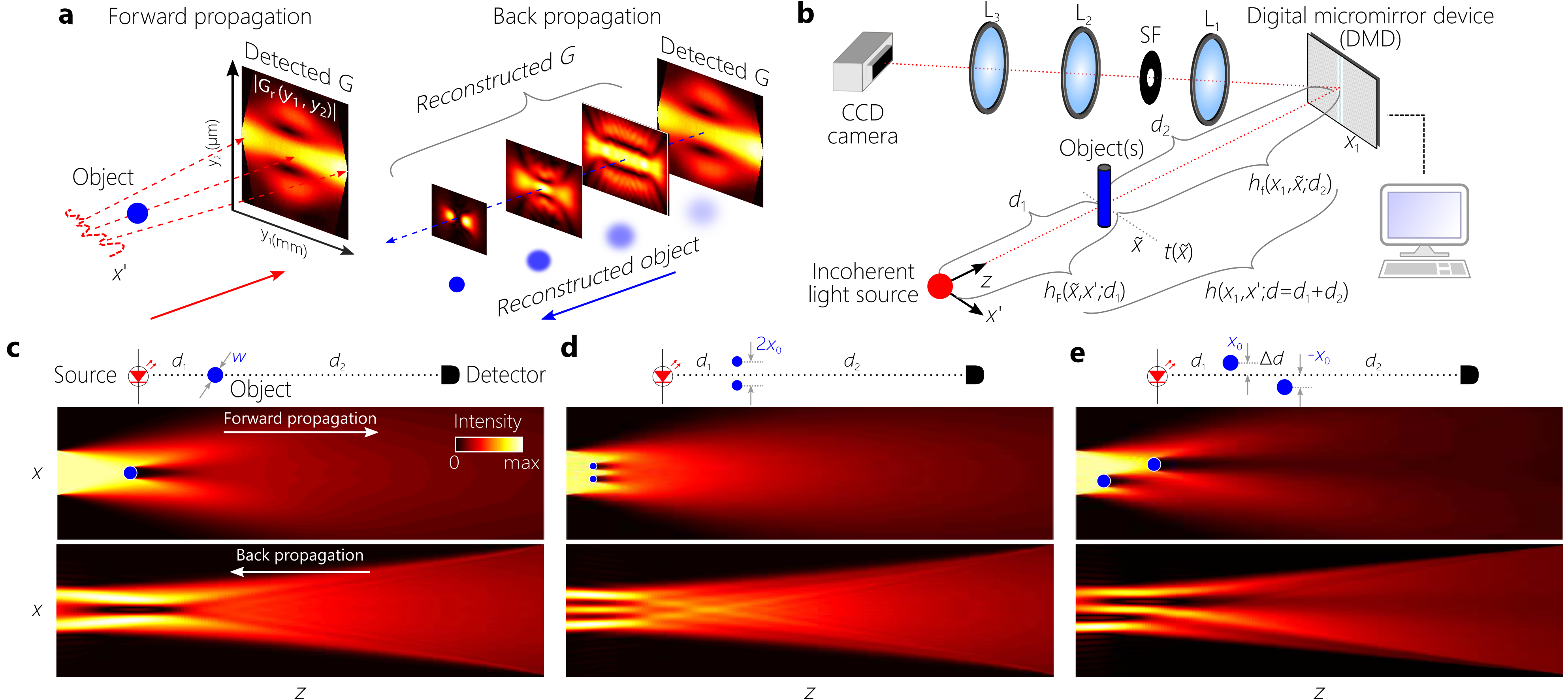 Figure 1
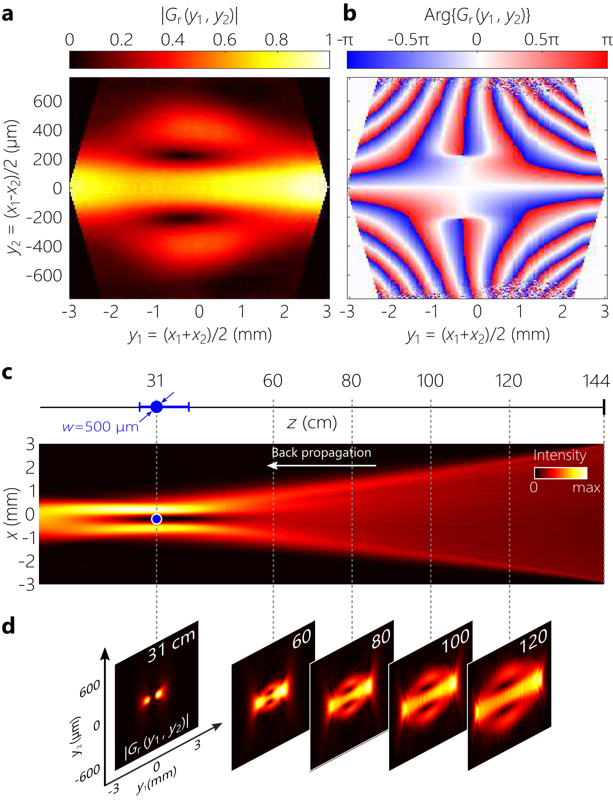 Figure 2
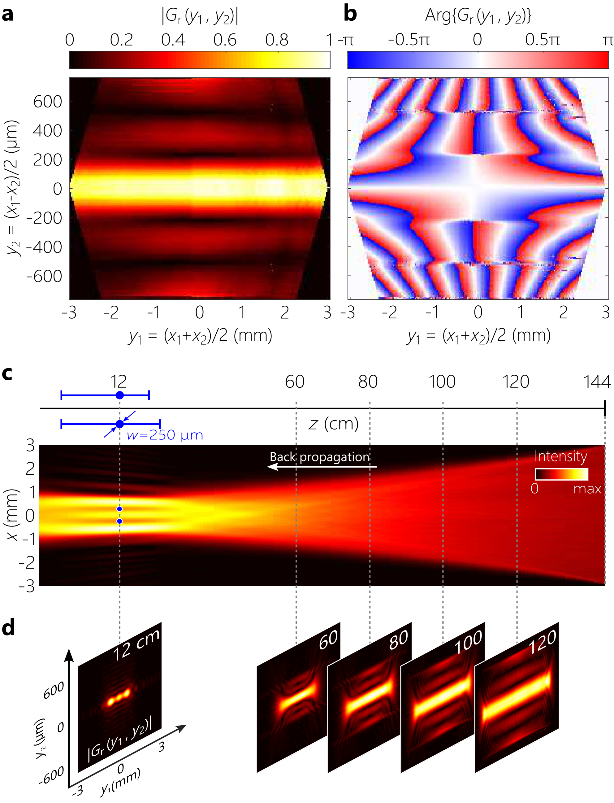 Figure 3
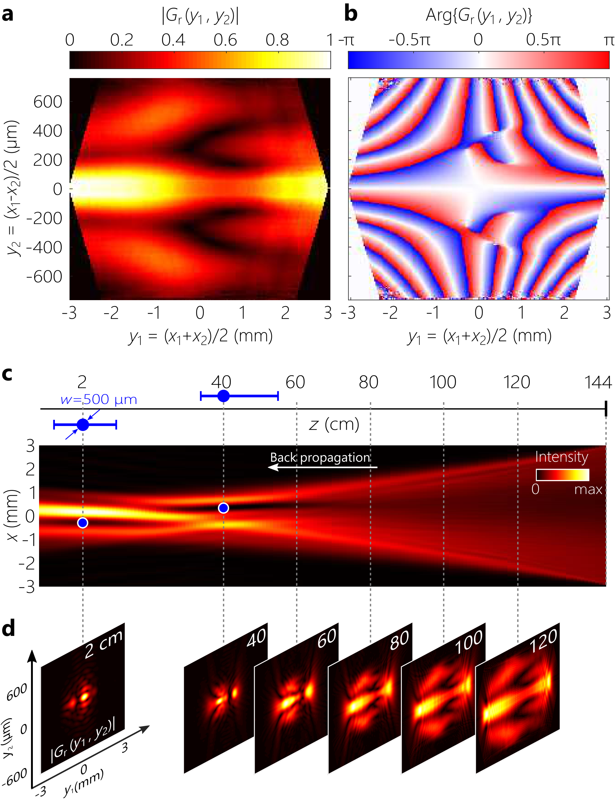 Figure 4
Peer Reviews
No public reviews on file for this paper yet. If you reviewed it on a platform where reviews are public (OpenReview, ICLR, NeurIPS, ICML), you can paste yours below so the community can read it here.
Videos
No videos yet. Explain this paper in a talk, walkthrough, or lecture? Add one.
††thanks: These two authors contributed equally††thanks: These two authors contributed equally
Incoherent lensless imaging via coherency back-propagation
Ahmed El-Halawany
CREOL, The College of Optics & Photonics, University of Central Florida, Orlando, Florida 32816, USA
Andre Beckus
Department of Electrical and Computer Engineering, University of Central Florida, Orlando, FL 32816, USA
H. Esat Kondakci
Morgan Monroe
Nafiseh Mohammadian
CREOL, The College of Optics & Photonics, University of Central Florida, Orlando, Florida 32816, USA
George K. Atia
Department of Electrical and Computer Engineering, University of Central Florida, Orlando, FL 32816, USA
Ayman F. Abouraddy
CREOL, The College of Optics & Photonics, University of Central Florida, Orlando, Florida 32816, USA
Abstract
The two-point complex coherence function constitutes a complete representation for scalar quasi-monochromatic optical fields. Exploiting dynamically reconfigurable slits implemented with a digital micromirror device, we report on measurements of the complex two-point coherence function for partially coherent light scattering from a ‘scene’ comprising one or two objects at different transverse and axial positions with respect to the source. Although the intensity shows no discernible shadows in absence of a lens, numerically back-propagating the measured complex coherence function allows estimating the objects’ sizes and locations – and thus the reconstruction of the scene.
The complex field amplitude associated with a coherent monochromatic scalar optical field provides a complete representation ( stands for the spatial coordinates) 1. Once the amplitude and phase of are measured – by digital holography 2; 3, acquiring the intensity in two planes 4; 5; 6; 7, or wavefront sampling 8, for example – the field can be computed in any other plane using the diffraction propagator. When spatially incoherent light scatters off an object, the far-field intensity no longer retains distinctive features. Although the transfer function representing free propagation of incoherent light has no zeros 9, it nevertheless decays sharply with spatial frequency, thus significantly diminishing the contrast of far-field intensity variations and reducing the potential of identifying a scattering object. However, the two-point field correlations for pairs of points and in a quasi-monochromatic scalar field at a wavelength provides a complete representation 10: determining at a plane allows evaluating it at any other plane. Measuring can be accomplished via wavefront sampling 11; 12 or lateral-shear interferometry 13; 14, among other possibilities 15; 16; 17; 18; 19; 20. Other approaches to incoherent lensless imaging of an object include interferometric tomography 21 and rotational-shear interferometry 22.
In this paper, we measure the coherence function of the optical field from an LED that is intercepted by a ‘scene’ comprising one or more obstacles. The partially coherent field evolves after the scene until intensity variations representative of the objects (shadows) are no longer discernible. The coherence function is measured by implementing dynamically reconfigurable double slits 23 using a digital micromirror device (DMD) 24. For simplicity, we consider fields with one transverse coordinate (assuming all fields are uniform along the other coordinate) and obtain the magnitude and phase of at the detection plane from the visibility of the interferogram and the shift of the central fringe with respect to a fixed reference, respectively 11, and then back-propagate towards the source to discover the scene and locate the scattering objects (we drop for convenience). We recently demonstrated that measuring along the axis helps identify the transverse location and subtended angle (object width divided by its distance to the detection plane) of a single scattering object 25. To identify the width and axial location separately, along with the transverse location, and – furthermore – to reconstruct a more complex scene, a measurement of the full coherence function becomes necessary – as we proceed to demonstrate.
The field correlations between two points and in a plane at a distance along the propagation axis can be described by a spatial coherence function , where is a realization of a stochastic electric field and indicates an ensemble average, with the intensity laying along the diagonal . Starting from a planar source having a coherence function , the coherence function at points and in a plane at after traversing a linear system having an impulse response function is
[TABLE]
Here, need not be unitary, so that systems including obstructions can be described in this way. In our experiments, comprises free-space propagation and interaction with opaque objects; see Fig. 1. Propagation a distance is represented with a Fresnel integral of kernel 1. In one configuration, comprises a sequence of free propagation a distance from the source, a thin opaque object represented by a transmittance , followed by propagation a distance to the detection plane [Fig. 1(a,b)]. This cascade is represented by the impulse response function
[TABLE]
and the coherence function at the detector is
[TABLE]
where is the coherence function immediately before the object. We also define a coherence function immediately after the object .
The specific form of the unitary operator for the Fresnel kernel 26 leads to the identity and a composition rule . By setting , becomes the inverse of : . Therefore, starting from the coherence function at the detector plane given in Eq. 3, we can back-propagate computationally a distance towards the object by applying the operator . When , the back-propagated coherence function becomes and the intensity , where is the intensity from the source immediately preceding the object.
Our strategy is thus to measure the complex coherence function and then carry out the back-propagation to reconstruct the scene. For convenience, we utilize a rotated coordinate system in lieu of , where and , such that . This basis rotation helps visualize and facilitates computing its evolution along by enabling a higher sampling efficiency in the -plane compared to that in the -plane. The intensity lies along the -axis , whereas the coherence properties are best gleaned along the -axis.
The coherence function is measured via dynamically reconfigurable double-slits implemented by a DMD (Texas Instrument DLP 6500) that has pixels with a pixel pitch of 7.56 m [Fig. 1(b)]. The width of each slit is m (3 pixels). The separation between the slits is varied in the range m, whereas their center spans the range mm with respect to the optical axis (DMD center) 25. Following the DLP is a imaging system (lenses L1 and L2 of focal lengths 10-cm and 20-cm, respectively, providing magnification) and a system comprising a spherical lens L3 of focal length 20 cm that produces interference patterns recorded by a CCD (The ImagingSource, DFK 31BU03), from which the magnitude and phase of are extracted 25; Fig. 1(b). The source is incoherent light from an LED (Thorlabs M625L3, peak wavelength of nm and FHWM-bandwidth nm) filtered through a 1.3-nm-bandwidth filter at a wavelength of 632.8 nm.
The experiment is initially carried out in absence of objects (unobstructed propagation from the ‘primary’ source to the detector) to calibrate the measurement system. The distance between the source and detector m is held fixed in all our experiments. We substitute the measured in the right-hand side of Eq. 1, replace by , and set the back-propagation distance to . A calibration phase is assessed that produces a maximum intensity profile at the source plane of the back-propagated signal. We now proceed to reconstructing ‘secondary’ sources – the scattering objects.
We first consider the case where an object (a metal wire of diameter mm at cm from the source) obstructs the field [Fig. 1(c)]. Diffraction after the object smears out the shadow, as predicted by a forward-model calculation [Fig. 1(c)] and confirmed in the measured [Fig. 2(a)]. By back-propagating the measured complex [Fig. 2(a,b)] and increasing the back-propagation distance , we construct the coherence function at planes preceding the detection plane axially and gradually approaching the object, samples of which are shown in Fig. 2(d). From we can extract the evolution of the intensity distribution along the propagation axis by setting at every plane [Fig. 2(d)]. Note the different scales along transverse (vertical) direction (4 mm) and longitudinal (horizontal) direction (1.44 m) in Fig. 2(c).
The back-propagation yields a localized ‘shadow’ of the object in the intensity profile that provides an estimate of the size and position (transverse and longitudinal) of the object [Fig. 2(c)]. For simplicity, we consider the ‘focal plane’ to be the plane in which the dip in the intensity profile reaches its minimum. The error in estimating the location of the object from the detection plane is . Note that the width of the intensity distribution decreases as we travel backwards and at the object plane is quite narrow; contrary to the extremely wide field produced from the LED. This is due to the finite size of the detection area: the source field far from the optical axis at the object plane does not contribute to the detection plane.
We next consider a scenario where two co-planar objects: two metal wires of equal diameters mm separated by mm and placed at a distance cm from the source [Fig. 3(a)]. The shadow cast by the two objects has mostly smeared out at the detector plane; see in Fig. 3(a). The measured complex [Fig. 3(a,b)] is back-propagated [Fig. 3(d)], and we extract the evolution of the intensity along the propagation axis as before [Fig. 3(c)]. The back-propagation yields two localized ‘shadows’ of the objects in the intensity profile from which we estimate the size and position of the two objects [Fig. 3(c)]. The error in estimating the location of the objects from the detection plane is .
Finally, we consider a scenario where two objects (metal wires of diameter mm each) are located in different planes along the propagation axis. The first object is at a distance cm from the source and is displaced to a position mm from the optical axis, and the second object follows it at a further distance along and is displaced to a symmetrically opposite transverse position [Fig. 1(e)]. Whereas the shadow cast by the first object (closest to the source) has mostly washed out, there is a remnant shadow from the second object (closest to the detection plane); see in Fig. 4(a). The measured complex [Fig. 4(a,b)] is back-propagated [Fig. 4(d)], and we extract the evolution of the intensity along the propagation axis as before [Fig. 4(c)]. Over the course of the back-propagation, two localized ‘shadows’ emerge. First, a shadow of the object closest to the detection plane emerges at cm in the intensity profile. We do not observe a shadow of the second object at this plane. By continuing the back-propagation procedure, the first observed shadow starts to smear out while a second shadow associated with the object closest to the source emerges. From these calculations, we can estimate the size and locations of the two objects [Fig. 4(c)]. The errors in estimating the location of the objects from the detection plane are and .
We now discuss some of the limitations of this approach. The back-propagation is exact only if the detector is of infinite size. The finite detector size leads to imperfections in reconstructing the scene; e.g., a finite resolution for distinguishing objects located at neighboring transverse or longitudinal positions. The results in Fig. 2 identify a limitation of this approach, namely that the region immediately behind the object (which is occluded from the perspective of the detector) represents a ‘null space’ for the procedure: a small object placed in the immediate vicinity behind the object will be difficult to observe. In general, when an object obstructs the light path, some information from the preceding planes is lost. For example, if two objects are placed in two different planes, the object closer to the detector will occlude the farther object. Finally, strictly speaking, the back-propagation procedure described above does not necessitate knowledge of the source for a successful reconstruction of the scene. We carried out a reference measurement for calibration only. An accurate measurement of suffices for the back-propagation procedure.
In conclusion, we have demonstrated that back-propagating the two-point complex coherence function measured in a plane can be utilized to reconstruct a scene containing scattering objects with no need for a lens. The coherence function need be measured at only one plane, even when the intensity in that plane lacks spatial variations indicative of the presence of objects. Acquiring the complex coherence function via wavefront sampling is made practical by utilizing a DMD that implements dynamically reconfigurable double slits. This work may be useful in imaging objects in turbid media where information lost in the intensity profile may still be glimpsed in the coherence domain.
Funding
Defense Advanced Research Projects Agency (DARPA), Defense Science Office under contract HR0011-16-C-0029.
Acknowledgments
We thank D. Mardani for suggesting improvements to the simulations. We also thank A. Tamasan, A. Dogariu, and A. Mahalanobis for helpful discussions.
The reference list from the paper itself. Each links out to its DOI / PubMed record.
- 1Saleh and Teich (2007) B. E. Saleh and M. C. Teich, Fundamentals of Photonics , 2nd ed. (Wiley-Interscience, 2007).
- 2Yamaguchi and Zhang (1997) I. Yamaguchi and T. Zhang, Opt. Lett. 22 , 1268 (1997).
- 3Kim (2011) M. K. Kim, Digital Holographic Microscopy (Springer, Berlin, 2011).
- 4Gerchberg and Saxton (1972) R. W. Gerchberg and W. O. Saxton, Optik 35 , 237 (1972).
- 5Fienup (1982) J. R. Fienup, Appl. Optics 21 , 2758 (1982).
- 6Abouraddy et al. (2006) A. F. Abouraddy, O. Shapira, M. Bayindir, J. Arnold, F. Sorin, D. S. Hinczewski, J. D. Joannopoulos, and Y. Fink, Nat. Mater. 5 , 532 (2006).
- 7Witte et al. (2014) S. Witte, V. T. Tenner, D. W. E. Noom, and K. S. E. Eikema, Light Sci. Appl. 3 , e 163 (2014).
- 8Vdovin et al. (2015) G. Vdovin, H. Gong, O. Soloviev, P. Pozzi, and M. Verhaegen, J. Opt. 17 , 1 (2015).