Exponential lower resolvent bounds far away from trapped sets
Kiril Datchev, Long Jin

TL;DR
This paper constructs examples of semiclassical Schrödinger operators with exponentially large resolvent norms far from trapped sets, revealing threshold radii where resolvent and wave decay behaviors change.
Contribution
It provides explicit radial examples demonstrating exponential resolvent growth far from trapped sets and analyzes the change in behavior at a critical radius.
Findings
Exponential lower bounds on resolvent norms far from trapped sets
Identification of a threshold radius affecting resolvent behavior
Application to wave equations showing change in decay properties
Abstract
We give examples of semiclassical Schr\"odinger operators with exponentially large cutoff resolvent norms, even when the supports of the cutoff and potential are very far apart. The examples are radial, which allows us to analyze the resolvent kernel in detail using ordinary differential equation techniques. In particular, we identify a threshold spatial radius where the resolvent behavior changes. We apply these results to wave equations with radial wavespeed, identifying a corresponding threshold radius at which wave decay properties change.
Click any figure to enlarge with its caption.
 Figure 1
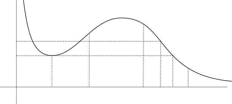 Figure 2
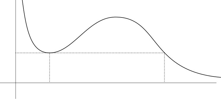 Figure 3
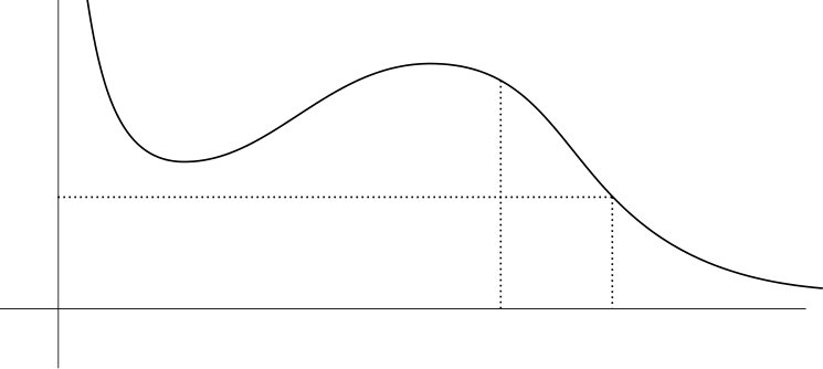 Figure 4
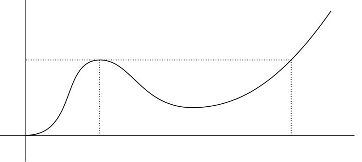 Figure 5
Peer Reviews
No public reviews on file for this paper yet. If you reviewed it on a platform where reviews are public (OpenReview, ICLR, NeurIPS, ICML), you can paste yours below so the community can read it here.
Videos
No videos yet. Explain this paper in a talk, walkthrough, or lecture? Add one.
Taxonomy
TopicsSpectral Theory in Mathematical Physics · Numerical methods in inverse problems · Advanced Mathematical Physics Problems
Exponential lower resolvent bounds far away from trapped sets
Kiril Datchev
Department of Mathematics, Purdue University, West Lafayette, IN, USA
and
Long Jin
Yau Mathematical Sciences Center, Tsinghua University, Beijing, China
(Date: July 6, 2018)
Abstract.
We give examples of semiclassical Schrödinger operators with exponentially large cutoff resolvent norms, even when the supports of the cutoff and potential are very far apart. The examples are radial, which allows us to analyze the resolvent kernel in detail using ordinary differential equation techniques. In particular, we identify a threshold spatial radius where the resolvent behavior changes. We apply these results to wave equations with radial wavespeed, identifying a corresponding threshold radius at which wave decay properties change.
The authors are very grateful to Semyon Dyatlov, Jeffrey Galkowski, Oran Gannot, Jason Metcalfe, Vesselin Petkov, Plamen Stefanov, and Maciej Zworski for helpful discussions. Thanks also to the anonymous referees for their comments and suggestions. KD was supported by the Simons Foundation through the Collaboration Grants for Mathematicians program, and by the National Science Foundation through grant DMS-1708511.
1. Introduction
In the first part of this paper we study semiclassical resolvent estimates, and in the second part we apply the results to wave decay and non-decay.
1.1. Semiclassical resolvent estimates
In this paper we investigate resolvent estimates for the semiclassical Schrödinger operator
[TABLE]
where , . Initially we suppose , but later we will relax this condition.
Question 1**.**
For which , and for which bounded and open sets , can we find an interval containing such that the incoming and outgoing cutoff resolvents obey
[TABLE]
for all sufficiently small?
It is well known that the answer depends upon dynamical properties of the classical flow in . Of particular importance is the trapped set at energy , which we denote ; this is the set of such that and is bounded as .
If is empty, that is to say if is nontrapping, then Robert and Tamura [RoTa1] show that the answer to Question 1 is that can be arbitrary. Analogous results hold in much more general nontrapping situations; see e.g. [Vo, HiZw] for some recent results, and see those papers and also [BoBuRa, Zw] for some pointers to the substantial literature on this topic.
But if is not empty, then Bony, Burq, and Ramond [BoBuRa] show that there is such that for any interval containing we have
[TABLE]
more specifically it is enough if contains an integral curve in . Moreover, as we discuss below, the right hand side can sometimes be replaced by .
Nevertheless, regardless of any trapping, for all there exists such that (1.1) holds whenever is disjoint from . Thus, if the distance between and is large enough, then all losses due to trapping are removed. This was first shown by Cardoso and Vodev [CaVo], refining earlier work of Burq [Bu2], and analogous results hold for much more general operators [CaVo, RoTa2, Vo, Da, DadH, Sh1].
It is not always necessary to cut off so far away: in [DaVa] it is shown that if trapping is sufficiently mild, then we have (1.1) whenever is disjoint from . (By ‘trapping is sufficiently mild’ we mean that the resolvent is polynomially bounded in ; see [DaVa] and also the survey [Zw, §3.2] and the book [DyZw, Chapter 6] for more details, including sufficient conditions on , and for references to some of the many known results of this kind.) Moreover, in that case (1.1) still holds if we replace by a microlocal cutoff vanishing only in a small neighborhood of in . If is normally hyperbolic, then the vanishing hypothesis can be weakened further: see [HiVa]. Propagation estimates play an important role in such results, and the connection between propagation estimates and polynomial resolvent bounds has been recently studied in [BoFuRaZe].
Our main result is that, when trapping is not mild, the situation can be dramatically different. Namely, losses due to trapping can show up very far away from the support of :
Theorem 1**.**
Suppose that is radial, , and . Let and let be a neighborhood of the sphere : see Figure 1. There is such that if
[TABLE]
then
[TABLE]
for all small enough.
The key point is that the distance between and (and hence, in particular, between and the trapped set ) can be arbitrarily large. This seems to be a new phenomenon.
Moreover, the conditions on and can be weakened, and in this nice radial setting we can say more. See Theorem 3 below for a stronger and more general result, and (4.11) for a more precise version of (1.3).
Lower bounds of the form (1.4) with stem from quasimodes, and they are well known to hold in radial situations or under a barrier assumption, namely when has a bounded connected component contained in . They have been recently investigated in [DaDyZw], where it is shown that, for satisfying a barrier assumption, can be replaced by , with only one of and containing . Lower bounds for the continuation of as crosses the positive real axis were recently studied in [BoPe, DyWa].
In the setting of Theroem 1, it is clear that no quasimodes can concentrate in because of the flow invariance of support of semiclassical measures. The quasimodes we use are concentrated in the set where is negative, and we show below (in Lemma 3) that their exponential decay away from this set is very slow. This is a key difference between our result and previous lower bounds as in [DaDyZw].
The form of the right hand side of (1.4) is essentially optimal: for any there is such that for any we have
[TABLE]
This was first shown by Burq [Bu1, Bu2] in a more general setting, and has been generalized still further in [CaVo, RoTa2, Vo, Da, DadH, Sh1, Ga].
We can define the value for more general potentials by
[TABLE]
As we mentioned previously, in [CaVo, RoTa2, Vo, Da, DadH, Sh1] it is shown that is finite for quite general and . In Theorem 1 we show that as for a family of examples, and in (4.11) we show that . Let us mention here that the finiteness of , in this setting as well as in more general ones, has been applied to a variety of problems in scattering theory: see e.g. [St, Mi1, GuHaSi, Ch]. There are also well-known consequences for Schrödinger and wave evolution: see §1.2 below. These applications motivate the following question.
Question 2**.**
What can we say about the value of for more general and ?
For example, it would be interesting to know if the hypothesis that is radial in Theorem 1 could be weakened. The lower bounds on resonance widths of [DaMa] make it seem unlikely that the radiality hypothesis could be removed altogether.
1.2. Wave decay and non-decay
We now give an application of the above results to decay and non-decay estimates for solutions to the wave equation with radial wavespeed, for simplicity restricting attention111See §1.4 for a discussion of why we do this. to the case . Thus, let be radial, so that , and suppose
[TABLE]
for some positive constants and . Given initial conditions , let be the solution to
[TABLE]
Then we have conservation of energy in :
[TABLE]
Our main result in this setting concerns energy on a bounded open set :
[TABLE]
This energy decays logarithmically in the sense that for all and there is such that
[TABLE]
In fact, these results are very robust. Proving the conservation of energy (1.8) is simple: one differentiates with respect to and integrates by parts, and so (1.8) clearly holds for very general symmetric operators. Proving the logarithmic decay (1.10) is more complicated, but it too has been established in great generality. The study of wave decay has a long history and we do not attempt to survey it here. We just mention that the first general logarithmic decay results are due to Burq [Bu1], and refer the reader also to [Bu2, Bo2, Mo, Ga, Sh2] for more recent results on logarithmic decay and for more references.
We now bring in an assumption which ensures (stable) trapping: namely we assume that
[TABLE]
Such a situation was considered by Ralston [Ra], who showed that then there are sequences of resonances converging exponentially quickly to the real axis, and it is well-known that in particluar this means (1.10) cannot be improved if contains the trapped set (see [HoSm, §7] for a recent version of such a result in the setting of general relativity). Note also that if instead we had then the problem would be nontrapping (see [Ra, p. 571].)
To state our result we will also need the threshold radius
[TABLE]
and we assume that
[TABLE]
Theorem 2**.**
Fix satisfying (1.7) and (1.13).
- (1)
If is disjoint from the closed ball , then there is such that
[TABLE]
for all . 2. (2)
If contains the sphere for some , then there is no such that (1.14) holds for all .
Remarks:
- (1)
One can check that (1.13) implies (1.11). We make the stronger assumption (1.13) because it simplifies our work, and because the most interesting examples have . 2. (2)
It is easy to construct families of examples such that with and fixed. One way is to take such that near [math] and put
[TABLE]
with . Then as . 3. (3)
We see that is a threshold at which wave decay behavior changes, just as in Theorem 3 we see that is a threshold at which resolvent norm behavior changes. Actually, by setting and we have (see §4 for more), and so is also a threshold for the behavior of the resolvent : see Lemma 6. 4. (4)
We expect that the second part of Theorem 2 can be strengthened to take into account a possible loss of derivatives as follows: if contains the sphere for some , then for any , there is no such that
[TABLE]
holds for all . (Thanks to Jason Metcalfe for suggesting this comment.)
We can interpret (1.14) as an ‘exterior’ wave decay estimate. Many variations of such estimates, including different types of smoothing and Strichartz estimates, have been established. See [BoTz, MaMeTa, MaMeTaTo, BuGuHa, Bo1, Mi2, ChWu, ChMe, RoTa2, MeStTa, BoChMePe] and references therein for results where behavior away from some compact set is better than behavior in sets which overlap trapping. Our result seems to give the first examples of ‘bad’ behavior extending arbitrarily far from the trapped set.
1.3. Outline of the rest of the paper
In §2 we state the main resolvent estimates of the paper, Theorem 3. In §3 we prove pointwise resolvent kernel bounds for a family of semiclassical ordinary differential operators, approximating the solutions by Airy functions using the remainder bounds of Olver [Ol]. In §4 we prove Theorem 3 and use it to prove Theorems 1 and 2.
1.4. Notation
In this paper is the Euclidean Laplacian on for some , is a (small) semiclassical parameter, is the characteristic function of , is a constant which may change from line to line, means that the closure of is a compact subset of , is the ball with center and radius , the sphere is its boundary, is the radial coordinate in , , and . and are Airy functions, see Appendix A.
The radius and wavespeed are defined in (1.7), and the radius is defined in (1.12). The potentials , , and are defined in (2.1) and the preceding sentences. The angular momentum and the radii and are defined in terms of the potential and the energy level in (2.2), (2.4), and (2.6) respectively: see also Figure 2 and Lemma 4 for more on these important quantities. The Schrödinger operator is defined in (3.1), its domain is defined in terms of the boundary condition immediately afterwards, and its resolvent kernel is then given in (3.2). We also sometimes use the domain given in (3.32). The angular momenta are defined in terms of the spherical eigenvalues in (4.2).
In §4.3 we use the homogeneous Sobolev space , defined to be the completion of with respect to the norm . When this is not a space of distributions and various technical difficulties arise (e.g. multiplication by a function in is not a bounded operator). For simplicity, in §1.2 and §4.3 we stick to the case (so that, in particular, Sobolev embedding implies ), but see [Sh2] for methods which cover the case . Note that in Theorems 1 and 3 these difficulties do not appear and we allow .
2. Main theorem
In this section we state our main semiclassical resolvent estimates. We begin with the assumptions, which are weaker but more complicated than the ones for Theorem 1.
Let , and let be radial, so that , and suppose222To keep things simpler while still capturing the interesting phenomena, one can restrict attention to the case . is bounded below and is bounded for all and .
Then is selfadjoint on a domain containing , and we fix such a domain. For we can define and study the incoming and outgoing resolvents using separation of variables as we recall in §4 below.
For , let
[TABLE]
This is the effective potential which arises when we write the Laplacian in polar coordinates; we think of as the angular momentum. For , put
[TABLE]
and suppose
[TABLE]
The trapping we use occurs at the angular momentum , and we will also need the following two radii. Put
[TABLE]
and suppose
[TABLE]
Put
[TABLE]
Note that if is compactly supported and , then the assumptions (2.3) and (2.5) are automatically satisfied for sufficiently small; we also have more explicit formulas for , , and , which we derive in §4.2 below. These assumptions imply that , so that the trapped set contains circular orbits in , and these are the trapped orbits that we will use (in Lemma 3) to prove exponential lower bounds. See Figure 2.
Theorem 3**.**
Let , , , and be as above.
If is bounded, open, and disjoint from a neighborhood of , then there is an interval containing and a constant such that
[TABLE]
for all small enough.
On the other hand, let and be bounded open sets in containing spheres and respectively, such that . Then there are constants and such that
[TABLE]
for all small enough. If in addition we have , then
[TABLE]
for tending to [math] along a sequence of positive values.
The main point is the value , which corresponds to from (1.6). Comparing (2.7) with (2.8) and (2.9) we see that is a threshold at which the behavior of the resolvent changes.
We now discuss the values of and , which come from Lemma 3 below. The former is related to an eigenvalue of an interior problem, and the latter to an Agmon distance, both for the effective potential . Such eigenvalues are known to approximate real parts of resonances near the real axis, while Agmon distances correspond to imaginary parts of the same resonances: see [HeSj] (especially §11 of that paper) and [FuLaMa] for results in a well-in-an-island setting, and [NaStZw, Corollary, §5] for an abstract statement. Let us emphasize that our lower bounds are in terms of an Agmon distance for rather than for , and the former may be much greater than the latter (for example, the latter vanishes if ). See also [Se] for one-dimensional resonance asymptotics using methods in some ways similar to ours, and [DaMa] for a more recent higher-dimensional result and more references.
An interesting special case is the one where has a unique local minimum, located at the origin, and moreover this minumum is nondegenerate and . Then , so that is a well-in-an-island type potential, and is at the bottom of the well. In that case, by [Na, Proposition 4.1], there is such that for any we have
[TABLE]
This upper bound shows that the form of the interval in (2.8) is optimal in general. See also [BoBuRa, §1] and [DaDyZw, §4] for further discussion.
3. Semiclassical ODE asymptotics
In this section we prove pointwise resolvent estimates, for energies near , for
[TABLE]
where is given by (2.1) with . Let be a domain for so that is selfadjoint and .
We briefly recall some facts about . By Proposition 2 and Theorems X.7, X.8, and X.10 of [ReSi, Appendix to X.I] we have , where is a boundary condition at [math] with real coefficients, and moreover unless . If , then we may have ; below we will not need further information about , but see [Re, BuGe] and [Ze, §10.4] for descriptions of the possibilities. Note finally that is preserved by complex conjugation because has real coefficients.
The outgoing resolvent kernel at energy is given by
[TABLE]
and it obeys , where and are certain solutions to
[TABLE]
and is their Wronskian. More specifically and satisfies , and is outgoing, that is to say it is asymptotic to a multiple of as . For convenience we assume without loss of generality that is real-valued.
In the remainder of §3 we prove three lemmas, each of which bounds for a different range of , , , and . The first two will be used to prove (2.7), and the third to prove (2.8) and (2.9).
In the first lemma is small enough that no turning point analysis is needed.
Lemma 1**.**
Fix , , and such that for all and . Then
[TABLE]
uniformly for all , , , and .
In §4 we will specify and ; they will be slightly larger than and respectively.
Before giving the proof we give the idea. We will use the fact that and are each oscillatory, rather than exponentially growing or decaying, since we are in the classically allowed region . So the upper bound follows from a lower bound on the Wronskian; this in turn follows from the fact that, roughly speaking, is like since it is outgoing, while is equal amounts and since it is real-valued.
Proof.
For any as above, by [Ol, §6.2.4] there are real constants and such that for we have
[TABLE]
where and satisfy
[TABLE]
when .
Again by [Ol, §6.2.4], we can normalize to be the outgoing solution of (3.3) given by
[TABLE]
for .
We compute the Wronskian
[TABLE]
where we dropped the remainder because is independent of . Combining this with (3.2), (3.5), and (3.7) gives (3.4). ∎
In the second lemma is large enough that a turning point analysis is needed. For our purposes the following bound which blows up near the turning point is sufficient, even though is of course continuous there. We state a result for all and , even though we only use a smaller range in our application, since the result for the full range is obtained with no extra effort. We remark that a closely related turning point analysis appears in a recent paper of Yafaev on semiclassical asymptotics for eigenfunctions in a potential well [Ya].
Lemma 2**.**
Fix such that for all , and fix containing such that for all and . Then
[TABLE]
uniformly for all , , and , where is given by (A.6).
Before giving the proof we give the idea. By rescaling, we can use as a new semiclassical parameter, and the turning point is roughly given by ; the classically forbidden region is and classically allowed region is . In the classically allowed region the bound holds for the same reason that it did in Lemma 1. In the classically forbidden region, the solutions are exponentially growing and decaying, rather than oscillatory, because there. But is forced to have only an exponentially decaying component and no exponentially growing one by the condition . Since we are estimating an expression of the form with , the decay from beats the growth from . The Wronskian cannot be very small for the same reason as in Lemma 1. Near the turning point these arguments break down, as can be seen from the weakness of (3.9) when or is close to .
Proof.
The proof proceeds in four steps. In the first we introduce some useful notation, including a change of variable in the manner of [Ol, §11.3]. In the second we express in terms of Airy functions, and compute asymptotics as and become large. In the third we do the same for , and in the fourth we compute the Wronskian and combine the previous results to conclude.
Put
[TABLE]
and note that
[TABLE]
see Figure 3.
Following [Ol, §11.3.1], we rewrite (3.3) as
[TABLE]
As we will see in (3.17) below, this decomposition leads to good asymptotic properties as .
Define an increasing bijection by
[TABLE]
Note that our differs from the one used in [Ol, §11.3] by a factor of .
We will need the following bound for : for sufficiently small we have
[TABLE]
By [Ol, §11.3.3], there are constants and such that
[TABLE]
where and are given by (A.1), and and satisfy
[TABLE]
and
[TABLE]
see Appendix B for more details. We use rather than in our definition of because this choice makes (3.17) hold uniformly for all , rather than merely uniformly on compact subintervals of : see Appendix B and also [Ol, §11.4.1 and §6.4.3].
Recalling that , and inserting (3.17), (A.2), and (A.3) into (3.15), we see that . Without loss of generality we normalize so that and
[TABLE]
We now derive the simpler and better asymptotics which hold for large ; these will ease the computation of the Wronskian later. If , then inserting (3.16) and (A.4) into (3.18) gives
[TABLE]
On the other hand, as in (3.5), there are real constants and such that for we have
[TABLE]
where and satisfy
[TABLE]
when . Setting (3.19) equal to (3.20) and applying (3.21) gives
[TABLE]
for large enough (depending on and ), where we used
[TABLE]
Hence
[TABLE]
Now we turn to . As in (3.7), we normalize it by setting
[TABLE]
for . Using [Ol, §11.3.3] again, there are constants and such that for we have
[TABLE]
Proceeding as in the proof of (3.22) gives
[TABLE]
Hence we have
[TABLE]
which implies
[TABLE]
We compute the Wronskian as in the proof of (3.8), and apply (3.23):
[TABLE]
Now (3.9) follows from inserting (3.18), (3.27), and (3.28) into (3.2), applying (3.16), (3.17), and (A.6), and observing that allows us to replace by in the final statement (actually, keeping gives a slightly better bound). ∎
In the third lemma the analysis is similar to that in the second, but slightly easier since we consider only a bounded range of . To obtain good lower bounds we consider only a particular energy level, rather than an interval of energies as in the previous two lemmas. We actually obtain an asymptotic, rather than merely a lower bound, with no extra effort.
Having information about in (3.30), rather than just , is important for our application to wave non-decay in Theorem 2, where we need a lower bound on .
Lemma 3**.**
Fix and fix . For any , there is an energy level , such that
[TABLE]
and
[TABLE]
where
[TABLE]
with . See Figure 4.
Moreover, it suffices to take to be an eigenvalue of as an operator on with domain
[TABLE]
Before giving the proof we give the idea. The operator has the same turning point behavior here as in Lemma 2, but this time we must take advantage of the trapping occuring at . We do this by finding an energy level which is also an eigenvalue of an interior problem (we use the Dirichlet problem on ) and then taking as the corresponding eigenfunction (this is our quasimode). This way both and grow exponentially in the classically forbidden region between and , giving the desired result.
Proof.
We begin by proving that has an eigenvalue as an operator on with domain . Note first that the spectrum of this operator is discrete since the domain is contained in , and let be the bottom of the spectrum. Then we have because by (2.2), the definition of . To see that , fix such that
[TABLE]
near , and let where is near and is supported inside the set where (3.33) holds. Then we have
[TABLE]
which concludes the proof that .
Let be a corresponding real-valued eigenfunction, and extend to solve (3.3) on all of .
Now we may again write in terms of Airy functions as in the proof of Lemma 2, with defined by (3.13), but now and are as in the statement of the present Lemma. The two main differences for our work here compared to that in the proof of Lemma 2 are that we have good remainder bounds only when , rather than for all , and that stays bounded.
More precisely, by [Ol, §11.3.3], there are real constants and such that for we have (3.15), where and satisfy (3.16) for and (3.17) for . We will need the following bounds on near the turning point :
[TABLE]
where we used .
Without loss of generality we normalize so that
[TABLE]
Since we have
[TABLE]
Now observe that by and (3.35) we have , and since , we obtain
[TABLE]
and combining with (3.36) gives
[TABLE]
When we have (3.20) with constants and , which we can compute as in (3.23) to find
[TABLE]
We take to be given by (3.24) for as before, where now (3.25) holds for with and given by (3.26). We now have (3.27) for . This time the Wronskian obeys
[TABLE]
where we used (3.38) and (3.37).
Inserting (A.2) and (A.3) into (3.15) and (3.25) and using (3.17) and (3.35) gives
[TABLE]
for , where . Then (3.30) follows from inserting (3.39) and (3.40) into (3.2) and using (3.26) and (3.37). We obtain (3.29) by the same argument with (3.24) in place of (3.40) for . ∎
4. Proofs of Theorems
4.1. Proof of Theorem 3
Let be the eigenvalues of the unit sphere of dimension , repeated according to multiplicity, and let be a corresponding sequence of orthonormal real eigenfunctions.
If is in the domain of , then
[TABLE]
where is given by (3.1) with
[TABLE]
Here is the usual surface measure on the unit sphere and for some as in §3.
Similarly, if is compactly supported, then so is and
[TABLE]
with the outgoing resolvent having integral kernel given by (3.2), and the incoming resolvent having integral kernel given by the complex conjugate of . (Actually, in (4.3) we could instead take in a weighted space but we will not need this.)
Hence if and are bounded and compactly supported functions on , then
[TABLE]
Proof of (2.8).
Suppose without loss of generality that . Then (2.8) follows from Lemma 3, applied with for any chosen such that , and with chosen such that for some and for some . ∎
Proof of (2.7).
Fix such that is disjoint from a neighborhood of . Fix and containing such that the hypotheses of Lemmas 1 and 2 are satisfied (it is enough if and the length of are sufficiently small). Then apply the Hilbert–Schmidt bound
[TABLE]
which holds uniformly for all . ∎
Finally, to prove (2.9), by Lemma 3 it suffices to show that is an eigenvalue of on , for some sequence such that obeys , for sufficiently large. This follows from a calculation very similar to that in (3.33) and (3.34), but note that now we will necessarily have ; this is reasonable because we are now assuming and hence by definition (2.2). We will first define the sequence , then prove that
[TABLE]
and then prove that
[TABLE]
We define for sufficiently large by demanding that be the bottom of the spectrum of
[TABLE]
as an operator on with domain
[TABLE]
Note that this operator is selfadjoint (that is, there is no need for an analogue of the condition as in the definition of in the beginning of §3) as long as , that is to say for all but possibly finitely many : see [Ze, Theorem 10.4.4] and also [ReSi, Theorem X.10]. The spectrum is discrete since the domain is contained . Also, will follow from (4.4). Hence, to show (2.9) it is enough to prove (4.4) and (4.5).
Proof of (4.4).
We have, for ,
[TABLE]
where we used the fact that by definition
[TABLE]
This implies and hence (4.4). ∎
Proof of (4.5).
Let , with as in (3.33) and as in the line after. Then, as in (3.34),
[TABLE]
This implies and hence (4.5). ∎
4.2. Proof of Theorem 1
To deduce Theorem 1 from 3, we begin with some useful formulas relating , , and . We define
[TABLE]
Lemma 4**.**
With the assumptions and notation of Theorem 3, we have
[TABLE]
[TABLE]
[TABLE]
[TABLE]
See Figure 5.
Proof.
To show (4.6) we compute
[TABLE]
and the right hand side is positive when by (2.5). To prove the other three statements we observe is the same as , with equality always holding simultaneously. ∎
Now suppose that is compactly supported in and . Then . If
[TABLE]
then , and we have moreover
[TABLE]
and
[TABLE]
as desired.
4.3. Proof of Theorem 2
It is convenient to work over the Hilbert space . Let
[TABLE]
Then is selfadjoint on with domain , and we will study the unitary wave propagator .
Theorem 2 follows from
Lemma 5**.**
Let and be as in Theorem 2.
- (1)
If has support disjoint from the closed ball , then there is such that
[TABLE]
for all . 2. (2)
If is positive on the sphere for some , then
[TABLE]
Indeed, to prove Theorem 2 from Lemma 5, we observe that if and near , then
[TABLE]
with , where for the first inequality we used Poincaré’s inequality
[TABLE]
To prove Lemma 5, we will need some facts about the resolvent of , based on the formula
[TABLE]
see [PoVo, p. 265], [Bu3, (2.13)], and [Sh2, (6.6)]. For any , the cutoff resolvent extends continuously from the lower, or upper, half plane to its closure, as an operator from to (see item 1 of [DadH, Lemma 4.1] for a proof using the Sjöstrand–Zworski black box theory [SjZw]). By (4.14) we see that has corresponding continuous extensions as an operator from to , and we denote these by , where .
Lemma 6**.**
Let and be as in Theorem 2.
- (1)
If has support disjoint from the closed ball , then there is such that
[TABLE]
for all . 2. (2)
If is positive on the sphere for some , then there are and a sequence such that
[TABLE]
Proof of Lemma 6.
We use the identity
[TABLE]
where and . To check this, note that if is compactly supported, and
[TABLE]
with and both outgoing, then (see [DyZw, Theorem 3.34 and Theorem 4.18]).
With and , we have, in the notation of Theorem 3 and Lemma 4, . Then
[TABLE]
and hence .
- (1)
By (2.7), for all having support disjoint from the closed ball , we have
[TABLE]
By a standard argument (see for example the proof of [Bu3, Proposition 2.4]), together with (4.14) this implies (4.15) for all such . 2. (2)
To prove (4.16), we argue similarly, but using the following refined version of (2.9):
[TABLE]
where is positive on the sphere for some , and is the same sequence appearing in (2.9). This refined version follows from (3.30) in the same way that (2.9) does, and it implies (4.16) with .
∎
Proof of Lemma 5.
This is a version of Kato smoothing [Ka]; see also [ReSi, §XIII.7] for another general presentation of the theory. We will use an argument as in [BuGéTz, §2.3] and [Bu3, §2]; see also [DyZw, §7.1]. We define the operator
[TABLE]
with adjoint
[TABLE]
Boundedness of from to is equivalent to boundedness of from to . We write
[TABLE]
Now let us suppose temporarily that there is such that
[TABLE]
so that in particular
[TABLE]
We use the equations
[TABLE]
to compute the Fourier–Laplace transforms
[TABLE]
where and . By Plancherel’s theorem,
[TABLE]
where we used (4.17) and (4.19), and where we allow the integrals to take the value . By density, (4.20) holds also without the assumption (4.18). Now (4.12) follows from (4.15).
To deduce (4.13) from (4.16), we must show that (4.16) implies
[TABLE]
But this is clear since is continuous by the discussion following (4.14) and unbounded by (4.16).
∎
Appendix A Airy functions
In this appendix we review some needed facts about the Airy functions given by
[TABLE]
These are solutions to satisfying , and as we have
[TABLE]
[TABLE]
[TABLE]
[TABLE]
These results can be found in [Ol, §11.1], among other places. In particular, there is a constant such that, for all real and satisfying , we have
[TABLE]
Appendix B Remainder bounds for Airy approximations
In this appendix we prove (3.16) and (3.17). By [Ol, Chapter 11, Theorem 3.1], it is enough to show that is uniformly bounded for all and , where
[TABLE]
with and as in (3.12) and
[TABLE]
We will first show that there is such that
[TABLE]
and then we will show that
[TABLE]
Proof of (B.3).
By Taylor’s theorem, for we have
[TABLE]
where we used and (these follow from (3.11)). Similar expansions hold for powers and derivatives of , and inserting the expansion for into (B.2) gives
[TABLE]
Hence
[TABLE]
[TABLE]
[TABLE]
Combining these and using gives
[TABLE]
which implies (B.3). ∎
Proof of (B.4).
To bound the first term in (B.4) we use
[TABLE]
and
[TABLE]
for . These imply
[TABLE]
for , which implies the bound on the first term in (B.4).
To bound the second term in (B.4), we use
[TABLE]
for (for the last term c.f. (3.14)), which implies
[TABLE]
Let , so that for we have
[TABLE]
for . Then, since , we have
[TABLE]
and inserting into (B.1) and combining with (B.6) gives the bound on the second term in (B.4). ∎
The reference list from the paper itself. Each links out to its DOI / PubMed record.
- 1[Bo Bu Ra] Jean-François Bony, Nicolas Burq, and Thierry Ramond, Minoration de la résolvante dans le cas captif . C. R. Math. Acad. Sci. Paris, 348:23–24 (2010), pp. 1279–1282.
- 2[Bo Fu Ra Ze] Jean-François Bony, Setsuro Fujiié, Thierry Ramond, and Maher Zerzeri, Propagation des singularités et résonances . C. R. Math. Acad. Sci. Paris, 355:8 (2017), pp. 887–891.
- 3[Bo Pe] Jean-François Bony and Vesselin Petkov, Semiclassical estimates of the cut-off resolvent for trapping perturbations . J. Spectr. Theory, 3:3 (2013), pp. 299–422.
- 4[Bo Ch Me Pe] Robert Booth, Hans Christianson, Jason Metcalfe, and Jacob Perry, Localized energy for wave equations with degenerate trapping . Math. Res. Lett. 26:4 (2019), pp. 991–1025.
- 5[Bo 1] Jean-March Bouclet, Strichartz estimates on asymptotically hyperbolic manifolds. Anal. PDE, 4:1 (2011), pp. 1–84.
- 6[Bo 2] Jean-Marc Bouclet, Low Frequency Estimates and Local Energy Decay for Asymptotically Euclidean Laplacians. Comm. Partial Differential Equations, 36:7 (2011), pp. 1239–1286.
- 7[Bo Tz] Jean-Marc Bouclet and Nikolay Tzvetkov, Strichartz estimates for long range perturbations . Amer. J. Math., 129:6 (2007), pp. 1565–1609.
- 8[Bu Ge] W. Bulla and F. Gesztesy, Deficiency indices and singular boundary conditions in quantum mechanics . J. Math. Phys., 26:10 (1985), pp. 2520–2528.