Energy statistics in open harmonic networks
Tristan Benoist, Vojkan Jak\v{s}i\'c, Claude-Alain Pillet

TL;DR
This paper investigates the long-term behavior of energy statistics in open harmonic networks, establishing a connection to the variance-gamma distribution and validating predictions with experimental data.
Contribution
It introduces a comprehensive analysis linking energy fluctuations in harmonic networks to the variance-gamma distribution and proves a full Large Deviation Principle.
Findings
Energy statistics follow a variance-gamma distribution asymptotically.
Theoretical predictions align with experimental data from electronic RC networks.
Large Deviation Principle is established for both Hamiltonian and stochastic dynamics.
Abstract
We relate the large time asymptotics of the energy statistics in open harmonic networks to the variance-gamma distribution and prove a full Large Deviation Principle. We consider both Hamiltonian and stochastic dynamics, the later case including electronic RC networks. We compare our theoretical predictions with the experimental data obtained by Ciliberto et al. [Phys. Rev. Lett. 110, 180601 (2013)].
Click any figure to enlarge with its caption.
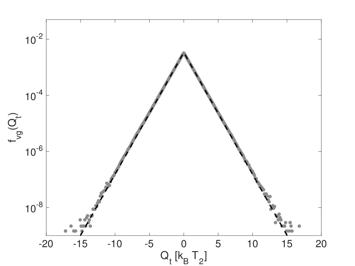 Figure 1
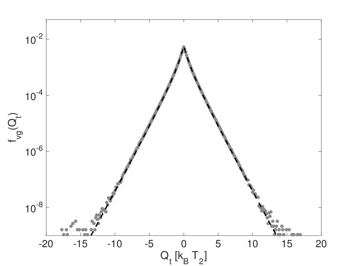 Figure 2
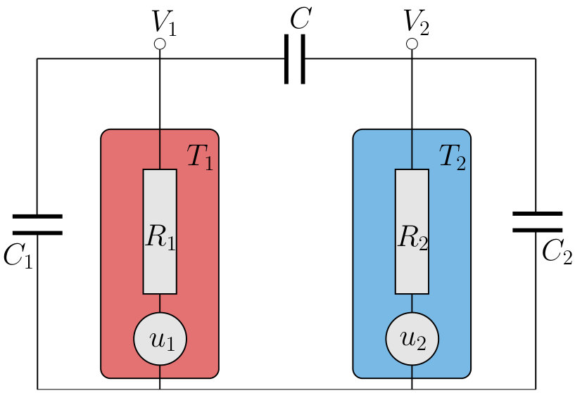 Figure 3
Peer Reviews
No public reviews on file for this paper yet. If you reviewed it on a platform where reviews are public (OpenReview, ICLR, NeurIPS, ICML), you can paste yours below so the community can read it here.
Videos
No videos yet. Explain this paper in a talk, walkthrough, or lecture? Add one.
Energy statistics in open harmonic networks
Tristan Benoist1, Vojkan Jakšić2, Claude-Alain Pillet3
1Institut de Mathématiques de Toulouse, Équipe de Statistique et Probabilités,
Université Paul Sabatier, 31062 Toulouse Cedex 9, France
2Department of Mathematics and Statistics, McGill University,
805 Sherbrooke Street West, Montreal, QC, H3A 2K6, Canada
3Aix Marseille Univ, Université de Toulon, CNRS, CPT, Marseille, France
Abstract. We relate the large time asymptotics of the energy statistics in open harmonic networks to the variance-gamma distribution and prove a full Large Deviation Principle. We consider both Hamiltonian and stochastic dynamics, the later case including electronic RC networks. We compare our theoretical predictions with the experimental data obtained by Ciliberto et al. [CINT].
1 Introduction
This note grew out of a set of remarks concerning energy fluctuations in thermal equilibrium for open harmonic Hamiltonian or stochastic networks made in [JPS1, JPS2] (see Remark 5 in Section 3.2 of [JPS1] and Remark 3.25 in Section 3.6 of [JPS2]) and our attempts to interpret the experimental results of [CINT] in this context. From a theoretical point of view, it turned out that for this very specific question one can go far beyond the large deviation results of [JPS1, JPS2] and the above mentioned remarks: one can compute the statistics of energy fluctuations in steady state network in a closed form in terms of the variance-gamma distribution. Equally surprisingly, for some specific electronic RC-circuit this statistics and the resulting variance-gamma distribution were precisely measured in experiments of Ciliberto, Imparato, Naert, and Tanase [CINT], although the result was not explicitly reported (the focus of the experiment was the measurement of the non-equilibrium entropy production statistics). The purpose of this note is to comment on the theoretical derivation of the heat and work statistics in harmonic networks and RC-circuits, and in the latter case compare the theoretical prediction with experimental results of [CINT].
To describe more precisely the line of thought that has led to this note, consider a stationary stochastic process , , and set
[TABLE]
Obviously, , where denotes expectation, and one may ask about order one fluctuations of . A standard way to approach the respective large deviations problem is to study the limit
[TABLE]
for in . Of course, if is almost surely bounded, then has no order one fluctuations and for all . However, in some physically important cases with unbounded , one has for and for , where the critical is finite. This was precisely the case in the above mentioned remarks in [JPS1, JPS2], where was related to the energy flux across a finite part of harmonic Hamiltonian network in thermal equilibrium. If the Large Deviations Principle for is controlled by the Legendre transform of , then for any open set ,
[TABLE]
where denotes the probability distribution of . The rigorous justification of this step in [JPS1, JPS2] required an application of a somewhat subtle extension of the Gärtner-Ellis theorem. The conclusion of the remarks is that a physically important quantity like energy variation per unit time in thermal equilibrium, which has expectation zero, may exhibit order one fluctuations due to the fact that the phase space space is unbounded.
The experimental results of [CINT] indicated that a similar phenomenon happens and can be precisely measured in a suitable electronic RC-circuit. In examining the connection we realized that the large deviation result (1.1) can be considerably refined and that one can express the large time statistics of the energy fluctuations in a finite part of an open harmonic network in closed form in terms of the variance-gamma distribution. That in turn reflected on the experimental findings of [CINT]. In their setting, the large time statistics of energy change turns into the large time statistics of the total power dissipated in the resistors and is also described by the variance-gamma distribution. This allowed us to compare the theoretical prediction of the variance-gamma distribution with the experimental results of [CINT]. The comparison is presented in Subsection 4.3. The theoretical prediction is nearly perfectly matched with experimental results.
Although the mathematical analysis presented in this note is elementary, the conclusions shed a new light on some important aspects of statistical mechanics of open system and can be viewed as a fine statistical characterization of the quantities entering the first law of thermodynamic for finite subsystems of extended harmonic systems. For example, we show that the total kinetic energy of a finite subsystem verifies a universal LDP (1.1) with . These points requires further study and we plan to return to them in the future.
The note is organized as follows. In Section 2 we review the derivation of the variance-gamma distribution and describe its basic properties. Hamiltonian harmonic networks are discussed in Section 3. Stochastic harmonic networks and electronic RC-circuits are discussed in Section 4.
Acknowledgments. We are grateful to Sergio Ciliberto and David Stephens for useful discussions. We also wish to thank Sergio Ciliberto for making available to us the raw data of the experiment reported in [CINT] which allowed one of us (T.B.) to analyze the data and plot the Figure 2 in Section 4.3. The research of T.B. was partly supported by ANR- 11-LABX-0040-CIMI within the program ANR-11-IDEX-0002-02 and by ANR contract ANR-14-CE25-0003-0. The research of V.J. was partly supported by NSERC. The work of C.-A.P. was partly funded by Excellence Initiative of Aix-Marseille University - A*MIDEX, a French “Investissements d’Avenir” programme.
2 Probabilistic setting
2.1 Variance-gamma distribution of Gaussian vectors
Let and be independent -valued Gaussian vectors with zero mean and covariance , and let be a matrix on . The probability distribution of the random variable
[TABLE]
is called variance-gamma distribution of the pair . We shall denote it by . Obviously,
[TABLE]
where denotes the standard (zero mean, unit covariance) Gaussian measure on and the matrix is given by
[TABLE]
In this subsection we shall compute the density of in terms of the modified Bessel functions of the second kind
[TABLE]
and the function
[TABLE]
where denote the repeated eigenvalues of the matrix (2.2).
Proposition 2.1
The density of is given by
[TABLE]
where denotes the Lebesgue measure on the unit sphere in .
Remark 1. Although this result is well-known, due to the lack of a convenient reference we give a proof below.
Remark 2. It follows immediately from the definition (2.3) that for and . Hence (2.4) implies that for . For in depth discussion of Bessel functions we refer the reader to Watson’s treatise [W]. In this note we shall make use of the following facts:
- (1)
The only singularity of is a logarithmic branching point at , with the leading asymptotics
[TABLE]
Moreover, the function is monotone decreasing. It follows that is a monotone decreasing function of satisfying
[TABLE] 2. (2)
For fixed the asymptotic expansion
[TABLE]
holds with and
[TABLE] 3. (3)
For half-integer , , one has
[TABLE]
where denotes the modified spherical Bessel function of the second kind
[TABLE]
Remark 3. If , where denotes the identity matrix on and , then the integrand in (2.4) is a constant and thus
[TABLE]
where is the area of .
Remark 4. In the special case and it follows from (2.7) and (2.6) that
[TABLE]
More generally, for , (2.4) reduces to
[TABLE]
with . Elementary manipulations lead to
[TABLE]
where
[TABLE]
Proof of Proposition 2.1. Setting and one has . Note that and are independent identically distributed Gaussian random vectors with zero mean and unit covariance. It follows that the characteristic function of can be written as
[TABLE]
Performing the Gaussian integral over and invoking the invariance of under orthogonal transformations further yields
[TABLE]
It follows that
[TABLE]
Performing the Gaussian integral over , we derive
[TABLE]
and passing to the spherical coordinates and we obtain
[TABLE]
The change of variable gives
[TABLE]
and comparison with (2.3) yields the result.
2.2 Variance-gamma distribution of a Gaussian process
Consider a stationary -valued Gaussian stochastic process , , with mean zero and covariance . Given a matrix on we set
[TABLE]
and denote by the law of .
Setting again and , , one has . The Gaussian random vectors and are identically distributed, with zero mean, but they do not need to be independent. To deal with this point we introduce the -matrix with entries
[TABLE]
and formulate
Assumption (A)
[TABLE]
Proposition 2.2
Suppose that (A) holds. Then weakly as . Moreover, this convergence is accompanied with the following Large Deviations Principle: for any open set ,
[TABLE]
where the rate function is given by
[TABLE]
Proof. In terms of the -valued random variable one has
[TABLE]
is Gaussian with mean zero and covariance
[TABLE]
where and are the matrices given by
[TABLE]
The characteristic function of is
[TABLE]
Assumption (A) gives that
[TABLE]
and comparing with (2.10) we deduce that for any ,
[TABLE]
The weak convergence then follows from Lévy’s continuity theorem.
To prove the LDP, it suffices to consider the case . If , then is an increasing function of and since has a strictly positive density, the weak convergence implies that
[TABLE]
for . Hence,
[TABLE]
and the result follows. So we may assume that . We consider the case , the other case is similar.
From the convergence (2.12) we infer that for large enough there exists such that
[TABLE]
Denoting by the Gaussian measure on with zero mean and covariance and setting
[TABLE]
it follows from (2.13) that
[TABLE]
for large enough . Further noticing that
[TABLE]
and as we conclude that it suffices to show that
[TABLE]
We proceed to prove (2.14).
Obviously,
[TABLE]
and from the asymptotic expansion (2.5) we infer that there is a constant such that for large enough, all , and all ,
[TABLE]
Since , the formula (2.4) and the upper bound in (2.15) give, for large ,
[TABLE]
from which the upper bound
[TABLE]
follows. To prove the corresponding lower bound, fix and pick a neighborhood of in such that
[TABLE]
Replacing integration over with integration over in (2.4), the lower bound in (2.15) gives
[TABLE]
from which we infer
[TABLE]
Taking we derive the result.
3 Hamiltonian harmonic networks
3.1 Setup
A Hamiltonian harmonic network is specified by a quadruple , where is a countable set describing vertices of the network, and are elements of describing the masses and frequencies of the oscillators, and is a non-negative bounded operator on describing the coupling between the oscillators. We denote by the matrix elements of w.r.t. the standard basis of .
We identify and with the induced multiplication operators on and assume that, as such, and are strictly positive111The operator acting on a Hilbert space is strictly positive whenever for all and some .. The finite energy configurations of the network are described by vectors in the Hilbert space
[TABLE]
where the pair describes the momenta and positions of the oscillators. The Hamiltonian of the network is
[TABLE]
which is the quadratic form associated to the linear map defined by
[TABLE]
is a bounded strictly positive operator on so that
[TABLE]
defines an inner product on . We denote by the Euclidean space equipped with this inner product.
The Hamilton equation of motion writes with
[TABLE]
Note that is a bounded skew-symmetric operator on . It follows that the finite energy trajectories of the network are described by the action of the one parameter group of orthogonal transformations of .
In the sequel we shall make use of the following dynamical assumption:
Assumption (B) The spectrum of the operator , acting on , is purely absolutely continuous
It follows from Assumption (B) that for all ,
[TABLE]
3.2 Internal and external work, heat
We fix a finite subset and define the total/kinetic/potential energy of the corresponding subnetwork by
[TABLE]
To avoid trivialities, we shall assume that there exists and such that .
The force acting on a vertex decomposes into an internal component
[TABLE]
and an external one
[TABLE]
The work done by the external forces over the time interval is equal to the change in internal energy of the subnetwork
[TABLE]
Adding to it the work done by the internal forces we get the total work done on the subnetwork which equals the change in its kinetic energy:
[TABLE]
The change in potential energy of the subnetwork is and it is the opposite of the work done by the internal forces,
[TABLE]
Thinking of the subnetwork as an open system connected to a reservoir, we can interpret Eq. (3.17) as a statement of the first law of thermodynamics: the increase of the internal energy of the subnetwork equals the amount of heat extracted from the reservoir.
3.3 The equilibrium case
In this subsection we assume that the network is in thermal equilibrium at temperature . This means that is a stationary Gaussian process over the Hilbert space with mean zero and covariance
[TABLE]
where is the Boltzmann constant.
Since
[TABLE]
Assumption (B) implies (recall (3.16)) that
[TABLE]
In the same way one shows that
[TABLE]
and so the process satisfies Assumption (A). Applying Proposition 2.2 to the quadratic form we infer that the increase in kinetic energy of the subnetwork converges in law, as , to the variance-gamma distribution of the pair . One easily shows that
[TABLE]
and so, by Remark 3, the limiting law has density (2.7) with and . The LDP that accompanies this convergence holds with the rate function
[TABLE]
Applying Proposition 2.2 to we deduce in the same way that the heat absorbed by the subnetwork over the time interval converges in law, as , to the variance-gamma distribution of the pair . In this case
[TABLE]
where and denote its restriction to with Dirichlet boundary conditions on the complement . The density of the limiting law is given by (2.4) and, in this case, depends on the details of the interaction. It is interesting to notice that, by Schur’s complement formula,
[TABLE]
so that the LDP for heat holds with rate function
[TABLE]
where .
3.4 The non-equilibrium case
Let
[TABLE]
be a finite partition of and
[TABLE]
the induced decomposition of Hilbert space . We restrict to by setting if and zero otherwise. This leads to (non-interacting) subnetworks . Suppose that the -th subnetwork is in thermal equilibrium at temperature , let be the corresponding covariance and set
[TABLE]
Suppose also that the full network was initially described by a Gaussian random field over with mean zero and covariance . The initial probability measure evolves under the interacting dynamics determined by and at time , is a Gaussian probability measure with mean zero and covariance
[TABLE]
Set
[TABLE]
where denotes the generator of the dynamics of the -th subnetwork. Assuming that is a trace class operator and that Condition (B) holds, a standard trace-class scattering argument [LS] gives that the strong limits
[TABLE]
exists. Hence,
[TABLE]
also exists and . The Gaussian measure over with mean zero and covariance is the non-equilibrium steady state of the network associated to the initial state determined by . Obviously, weakly as .
One can now repeat the analysis of the previous section for the stationary Gaussian process with mean zero and covariance . Both the change in kinetic and total energy of a finite subnetwork converge in law to a variance-gamma distribution as . However, in this case there is no simple expression for the ’s. These eigenvalues depend on detailed dynamical properties of the model encoded in the scattering matrix . Even in the simplest example of a harmonic crystal analyzed in [JPS2, Section 3.2], not much is known about the ’s outside perturbative regimes.
4 Stochastic networks
4.1 Preliminaries
In this section we shall consider -valued Gaussian stochastic processes that arise as solutions of SDE’s of the form
[TABLE]
where and are and matrices and a standard -valued Wiener process. The solution of the Cauchy problem (4.19) with initial condition is
[TABLE]
We shall assume that is stable, that is, that all its eigenvalues have strictly negative real part, and set
[TABLE]
Note that is non-negative and satisfies the Lyapunov equation
[TABLE]
The pair is called controllable if the smallest -invariant subspace that contains is equal to . If is controllable, then and the centered Gaussian measure on with covariance is the unique stationary measure for the process . Moreover
[TABLE]
satisfies Assumption (A).
We now turn to two examples of the above framework: stochastic harmonic networks and stochastic RC-circuit.
4.2 Stochastic harmonic networks
We start with a Hamiltonian harmonic network where the vertex set is assumed to be finite. To each we associate two parameters describing a thermal reservoir coupled to the oscillator at : the temperature and the relaxation rate ( meaning: no reservoir attached to ). The external force acting on the oscillator at has the usual Langevin form
[TABLE]
where the are independent standard white noises. The equation of motion of stochastic network is
[TABLE]
With and obvious notation it can be cast to the form (4.19) with
[TABLE]
The matrix is stable and we shall assume that the pair is controllable. Distributing according to the centered Gaussian measure with covariance given by (4.20) yields a stationary Gaussian process satisfying Assumption (A). Note that in the equilibrium case, for all , is given by (3.18) which is now a finite matrix.
The variations of the total/kinetic energy of the network can be analyzed in the same way as in Subsections 3.3 and 3.4. In particular, in both cases one has the convergence in law to an appropriate variance-gamma distribution. The advantage of the stochastic setting over the Hamiltonian setting described in Section 3 is that the covariances are finite-dimensional matrices and thus accessible to numerical computations. In some important examples they can be explicitly computed. In the next subsection we analyze one such example.
4.3 Stochastic RC-circuit
The RC-circuit subject of the experimental investigations of [CINT] is described in Figure 1. We set
[TABLE]
The circuit analysis gives that the voltages satisfy the SDE
[TABLE]
where and . One easily verifies that the matrix is stable and that the pair is controllable. The stochastic term is due to Nyquist’s thermal noise in the resistors. We denote by and the powers dissipated in the resistances and at time . They satisfy, in Stratonovich sense,
[TABLE]
We are interested in the total dissipated power defined by
[TABLE]
where we set . By direct integration,
[TABLE]
The eigenvalues of
[TABLE]
can be computed by diagonalizing and evaluating the integral. The eigenvalues are given by
[TABLE]
where
[TABLE]
Recalling Remark 4 after Proposition 2.1, we can now complete the theoretical analysis of the total dissipated power.
Thermal equilibrium case . Then and it follows from Proposition 2.2 and Eq. (2.8) that converges in law as to the probability distribution with density
[TABLE]
Non-equilibrum case . Then and Proposition 2.2 and Eq. (2.9) yield that converges in law as to the probability distribution with density
[TABLE]
where
[TABLE]
[TABLE]
Figure 2 summarizes the comparison of these theoretical predictions with the experimental data from [CINT].
The reference list from the paper itself. Each links out to its DOI / PubMed record.
- 1[CINT] Ciliberto, S., Imparato, A., Naert, A., Tanase, M.: Heat flux and entropy produced by thermal fluctuations. Phys. Rev. Lett. 110 , 180601 (2013).
- 2[JPS 1] Jakšić, V., Pillet, C-A., Shirikyan, A.: Entropic fluctuations in thermally driven harmonic networks. J. Stat. Phys. 166 , 926–1015 (2017).
- 3[JPS 2] Jakšić, V., Pillet, C-A., Shirikyan, A.: Entropic Fluctuations in Gaussian Dynamical Systems. Rep. Math. Phys. 77 , 335–376 (2016).
- 4[LS] Lebowitz, J.L., Spohn, H.: Stationary non-equilibrium states of infinite harmonic systems. Commun. Math. Phys. 54 , 97–120 (1977).
- 5[W] Watson, G.N.: A Treatise on the Theory of Bessel Functions. (2nd. ed.). Cambridge University Press, Cambridge, 1966.