Convergence of eigenvector empirical spectral distribution of sample covariance matrices
Haokai Xi, Fan Yang, and Jun Yin

TL;DR
This paper establishes improved convergence rates for the eigenvector empirical spectral distribution of sample covariance matrices to the deformed Marčenko-Pastur law, under weaker moment conditions and more general matrix models.
Contribution
It provides sharper convergence rate bounds for VESD to the deformed MP distribution, extending previous results to broader settings with weaker assumptions.
Findings
Expected VESD converges to deformed MP law at rate N^{-1+ε}.
Almost sure convergence rate of VESD is improved to N^{-1/2+ε}.
Results hold under finite 6th and 8th moment conditions, with general covariance matrices.
Abstract
The eigenvector empirical spectral distribution (VESD) is a useful tool in studying the limiting behavior of eigenvalues and eigenvectors of covariance matrices. In this paper, we study the convergence rate of the VESD of sample covariance matrices to the deformed Mar\v{c}enko-Pastur (MP) distribution. Consider sample covariance matrices of the form , where is an random matrix whose entries are independent random variables with mean zero and variance , and is a deterministic positive-definite matrix. We prove that the Kolmogorov distance between the expected VESD and the deformed MP distribution is bounded by for any fixed , provided that the entries have uniformly bounded 6th moments and for some constant . This result improves the previous…
Click any figure to enlarge with its caption.
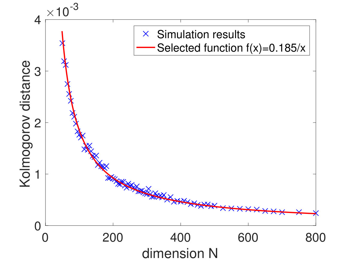 Figure 1
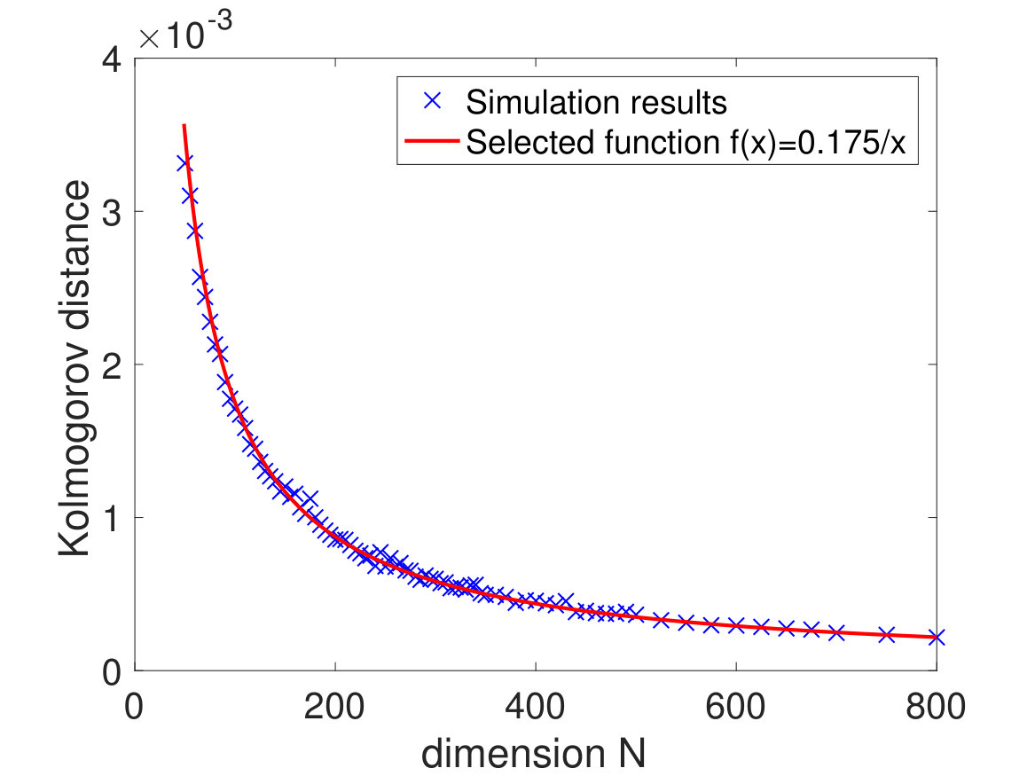 Figure 2
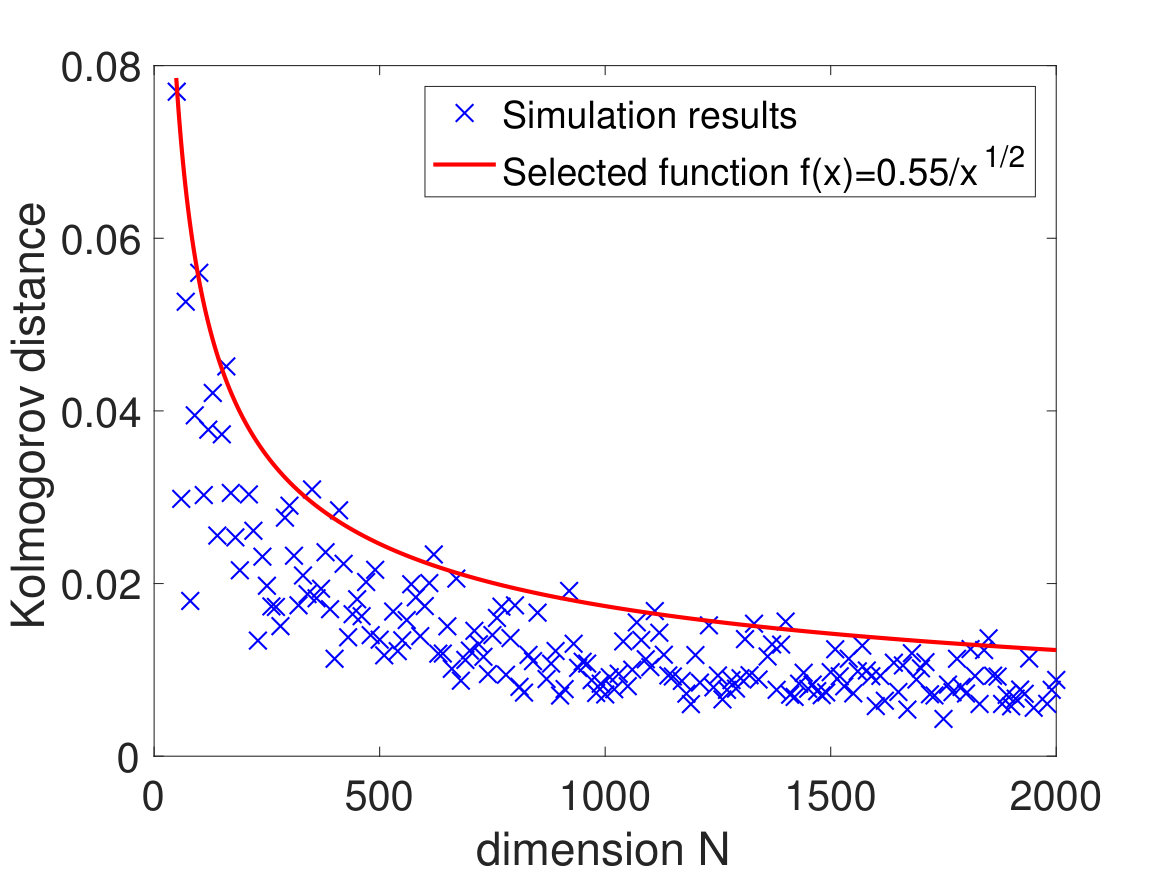 Figure 3
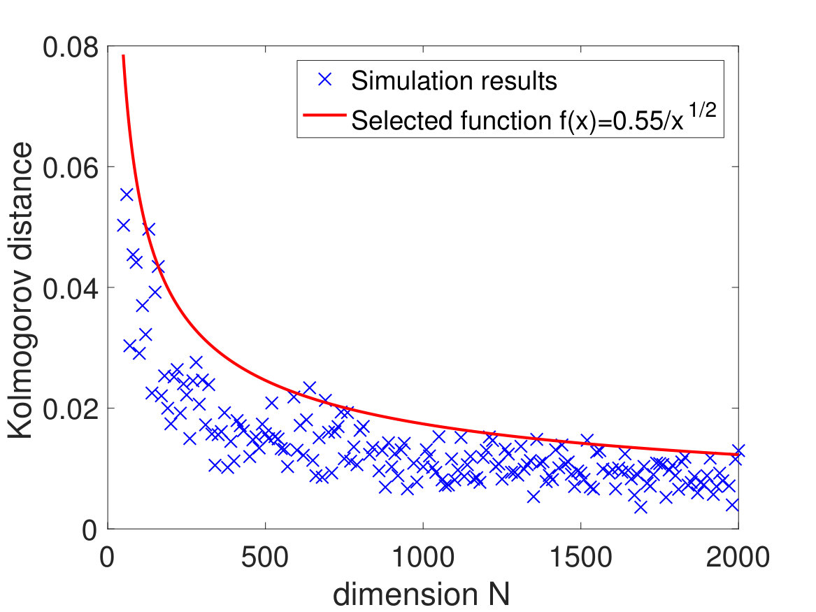 Figure 4
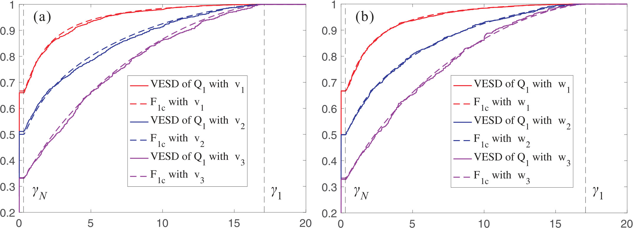 Figure 5
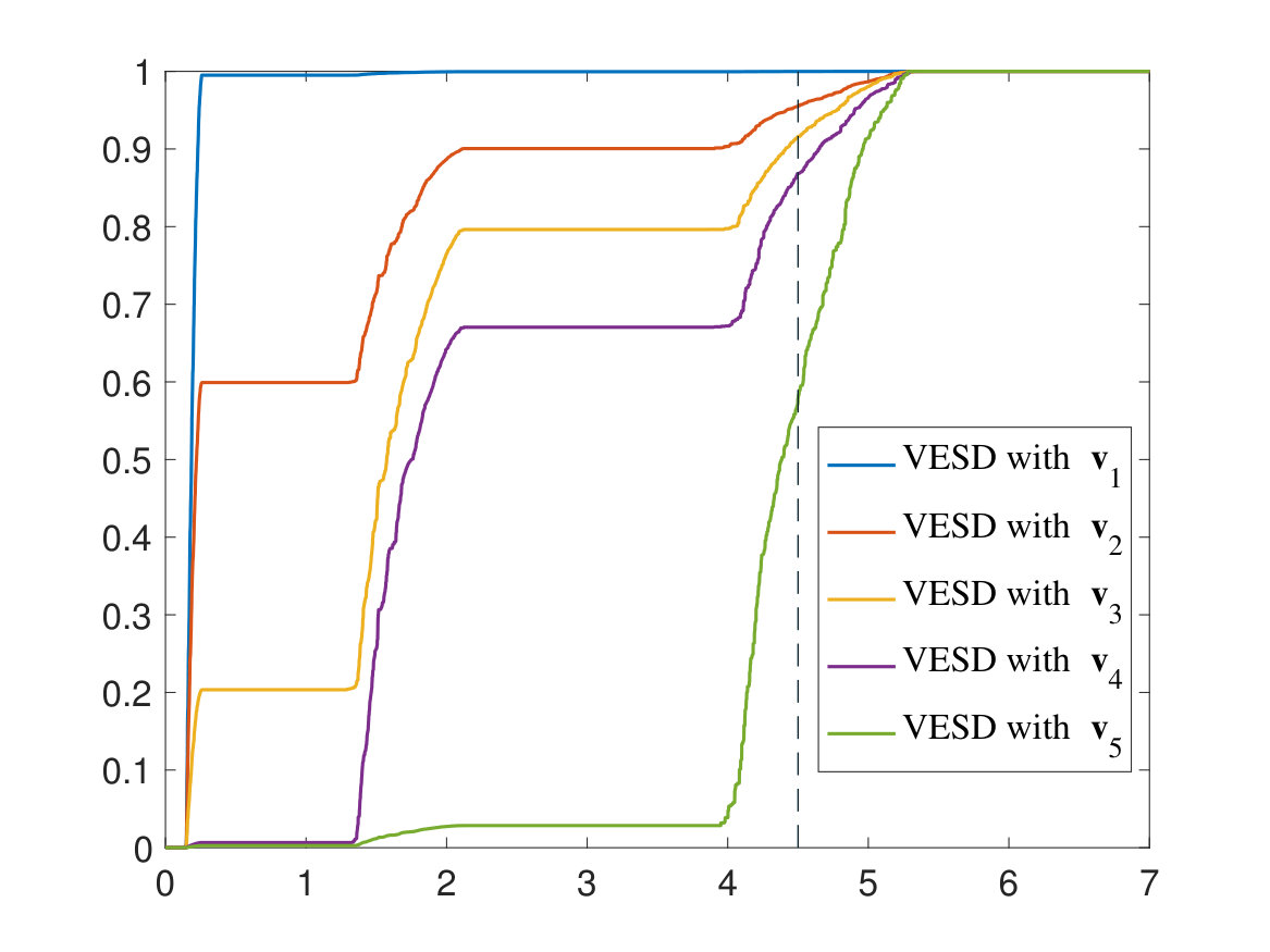 Figure 6
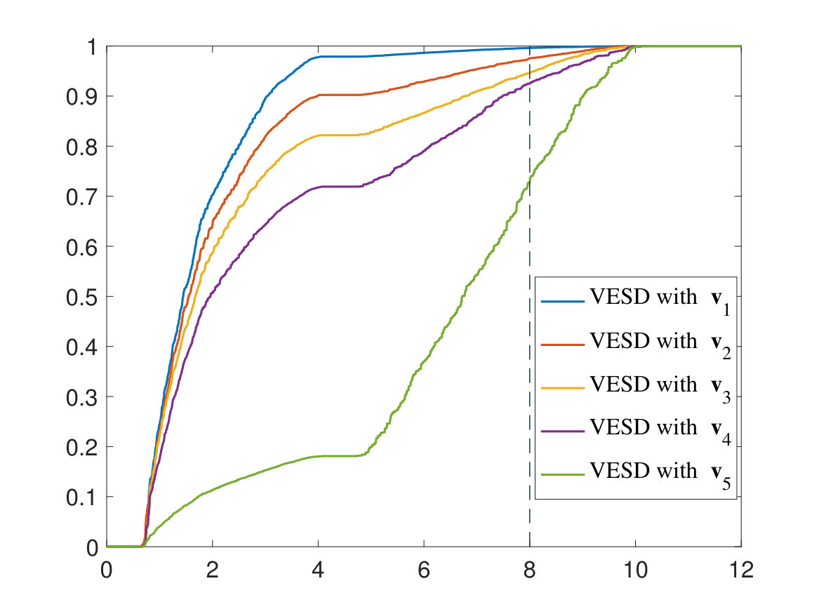 Figure 7
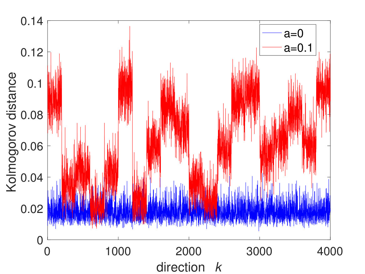 Figure 8
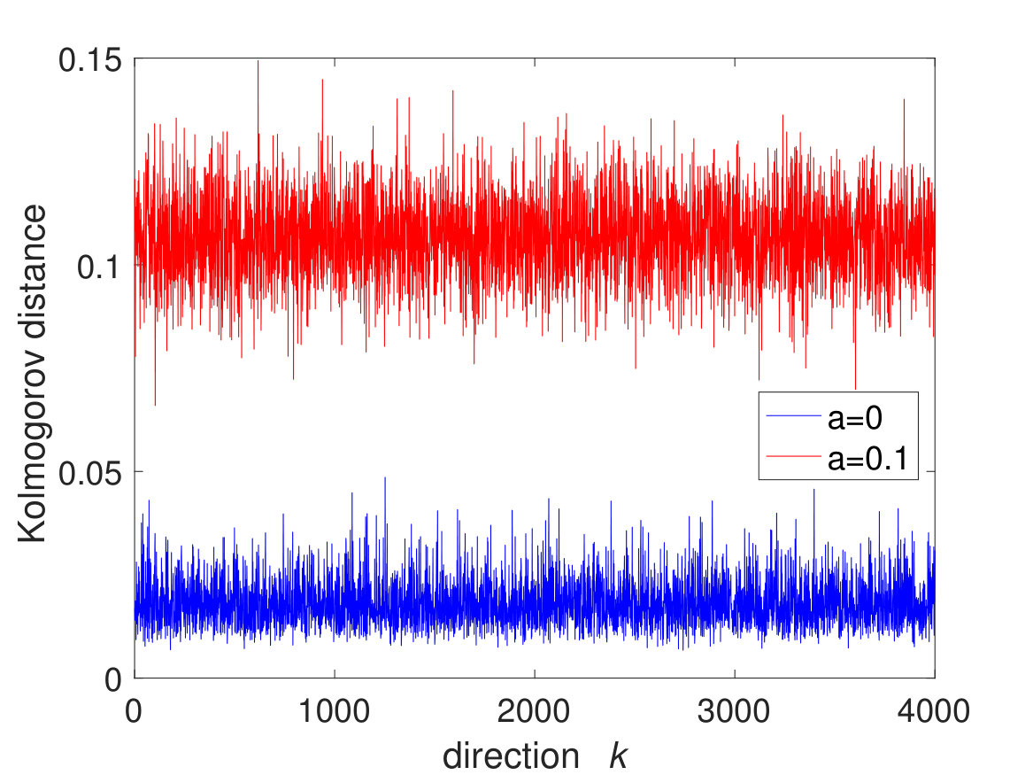 Figure 9
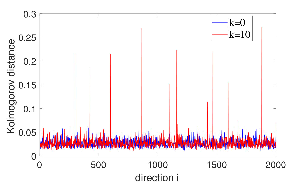 Figure 10
Peer Reviews
No public reviews on file for this paper yet. If you reviewed it on a platform where reviews are public (OpenReview, ICLR, NeurIPS, ICML), you can paste yours below so the community can read it here.
Videos
No videos yet. Explain this paper in a talk, walkthrough, or lecture? Add one.
Convergence of eigenvector empirical spectral distribution of sample covariance matrices
Haokai Xi label=e1][email protected] [
Fan Yang label=e2][email protected] [
Jun Yin label=e3][email protected] [ University of Wisconsin-Madison\thanksmarkm1 and University of California, Los Angeles\thanksmarkm2
Department of Mathematics
University of California, Los Angeles,
Los Angeles, CA 90095,
USA
E-mail: e3
Department of Mathematics
University of Wisconsin-Madison
Madison, WI 53706
USA
Abstract
The eigenvector empirical spectral distribution (VESD) is a useful tool in studying the limiting behavior of eigenvalues and eigenvectors of covariance matrices. In this paper, we study the convergence rate of the VESD of sample covariance matrices to the deformed Marčenko-Pastur (MP) distribution. Consider sample covariance matrices of the form , where is an random matrix whose entries are independent random variables with mean zero and variance , and is a deterministic positive-definite matrix. We prove that the Kolmogorov distance between the expected VESD and the deformed MP distribution is bounded by for any fixed , provided that the entries have uniformly bounded 6th moments and for some constant . This result improves the previous one obtained in [52], which gave the convergence rate assuming entries, bounded 10th moment, and . Moreover, we also prove that under the finite th moment assumption, the convergence rate of the VESD is almost surely for any fixed , which improves the previous bound in [52].
15B52,
62E20,
62H99,
Sample covariance matrix,
Empirical spectral distribution,
Eigenvector empirical spectral distribution,
Marčenko-Pastur distribution,
keywords:
[class=MSC]
keywords:
\startlocaldefs\endlocaldefs
,
and
T1Supported by NSF Career Grant DMS-1552192 and Sloan fellowship.
1 Introduction and main results
Sample covariance matrices are fundamental objects in multivariate statistics. The population covariance matrix of a centered random vector is . Given independent samples of , the sample covariance matrix is the simplest estimator for . In fact, if is fixed, then converges almost surely to as . However, in many modern applications, the advance of technology has led to high dimensional data where is comparable to or even larger than . In this setting, cannot be estimated through directly, but some properties of can be inferred from the eigenvalue and eigenvector statistics of . The large dimensional covariance matrices have more and more applications in various fields, such as statistics [13, 26, 27, 28], economics [40] and population genetics [41].
In this paper, we consider sample covariance matrices of the form , where is an real or complex data matrix whose entries are independent (but not necessarily identically distributed) random variables satisfying
[TABLE]
and the population covariance matrix , , is a deterministic positive-definite matrix. If the entries of are complex, then we assume in addition that
[TABLE]
Define the aspect ratio We are interested in the high dimensional case with . We will also consider the matrix , which share the same nonzero eigenvalues with .
A simple but important example is the sample covariance matrix with (i.e. the null case). In applications of spectral analysis of large dimensional random matrices, one important problem is the convergence rate of the empirical spectral distributions (ESD). It is well-known that the ESD of converges weakly to the Marčenko-Pastur (MP) law [36]. One way to measure the convergence rate of the ESD is to use the Kolmogorov distance
[TABLE]
The convergence rate for sample covariance matrices was first established in [2], and later improved in [23] to in probability under the finite 8th moment condition. In [44], the authors proved an almost optimal bound that with high probability for any fixed under the sub-exponential decay assumption.
The research on the asymptotic properties of eigenvectors of large dimensional random matrices is generally harder and much less developed. However, the eigenvectors play an important role in high dimensional statistics. In particular, the principal component analysis (PCA) is now favorably recognized as a powerful technique for dimensionality reduction, and the eigenvectors corresponding to the largest eigenvalues are the directions of the principal components. The earlier work on the properties of eigenvectors goes back to Anderson [1], where the author proved that the eigenvectors of the Wishart matrix are asymptotically normal and isotropic when is fixed and . For the high dimensional case, Johnstone [27] proposed the spiked model to test the existence of principal components. Then Paul [42] studied the directions of eigenvectors corresponding to spiked eigenvalues. In [35], Ma proposed an iterative thresholding approach to estimate sparse principal subspaces in the setting of a high-dimensional spiked covariance model. Using a reduction scheme which reduces the sparse PCA problem to a high-dimensional multivariate regression problem, [11] established the optimal rates of convergence for estimating the principal subspace for a large class of spiked covariance matrices. One can see the references in [11, 35] for more literatures on sparse PCA and spiked covariance matrices.
For the test of the existence of spiked eigenvalues, we first need to study the properties of the eigenmatrices in the null case. If , then the eigenmatrix is expected to be asymptotically Haar distributed (i.e. uniformly distributed over the unitary group). However, formulating the terminology “asymptotically Haar distributed” is far from trivial since the dimension is increasing. Following the approach in [46, 47, 3, 51, 52], we will use the eigenvector empirical spectral distribution (VESD) to characterize the asymptotical Haar property. Suppose
[TABLE]
is a singular value decomposition of , where
[TABLE]
are the left-singular vectors, and are the right-singular vectors. Then for deterministic unit vectors and , we define the VESD of as
[TABLE]
Now we apply the above formulations to the null case. Adopting the ideas of [46, 47], we define the stochastic process as
[TABLE]
If the eigenmatrix of is Haar distributed, then the vector is uniformly distributed over the unit sphere, and would converge to a Brownian bridge by Donsker’s theorem. Thus the convergence of to a Brownian bridge characterizes the asymptotical Haar property of the eigenmatrix. For convenience, we can consider the time transformation
[TABLE]
Thus the problem is reduced to the study of the difference between the VESD and the ESD. It was already proved in [3, 9] that also converges weakly to the MP law for any sequence of unit vectors . On the other hand, compared with ESD, much less has been known about the convergence rate of the VESD. The best result so far was obtained in [52], where the authors proved that if and the entries of are centered random variables, then under the finite 10th moment assumption, and almost surely under the finite 8th moment assumption. However, we find that both of these bounds are far away from being optimal, and can be improved with a different method. This is one of the purposes of this paper.
We will also extend the above formulation to include sample covariance matrices with general population . For a non-scalar , the eigenmatrix of is not asymptotically Haar distributed anymore. For its distribution, we conjecture that the eigenvectors of are asymptotically independent, and each is asymptotically normal with covariance matrix given by some . In fact, our results in this paper suggest that takes the form , where is defined in (1.15) to denote the classical location for , and is a matrix-valued function defined in (1.18) with the property that is the asymptotic distribution of the VESD for any . Again, since the dimension increases to infinity, the above property is hard to formulate. One way is to consider the finite-dimensional restriction in the following sense: given , for any fixed unit vector and , we should have asymptotically
[TABLE]
(In fact, for a nice choice of in the sense of Definition 1.2, is typically of order .) We can also adopt the approach as above, that is to investigate the stochastic process
[TABLE]
If , we conjecture that converges to the following Gaussian process for :
[TABLE]
where is a standard Brownian motion, is the asymptotic ESD of defined in (1.12), and denotes the quantile function. As before, we can study the process (1.6) through the time transformaton , where is the ESD of . Due to the rigidity of eigenvalues (see Theorem 3.7), we have for all ,
[TABLE]
with very high proability for any fixed . Thus we need to study the convergence rate of to , and this is our main goal. In fact, we will prove that the convergence rate of is for any fixed , which shows that the limiting process is centered, and the convergence rate of is , which partially verify the scaling.
1.1 Main results
We consider sample covariance matrices with a general diagonal , whose empirical spectral distribution is denoted by
[TABLE]
We assume that there exists a small constant such that
[TABLE]
The first condition means that the operator norm of is bounded, and the second condition means that the spectrum of cannot concentrate at zero. If converges weakly to some distribution as , then it was shown in [36] that the ESD of converges in probability to some deterministic distribution, which is called the deformed Marčenko-Pastur law. For any , we describe the deformed MP law through its Stieltjes transform
[TABLE]
We define as the unique solution to the self-consistent equation
[TABLE]
subject to the conditions that and for . It is well known that the functional equation (1.10) has a unique solution that is uniformly bounded on under the assumption (1.9) [36]. Letting , we can recover the asymptotic eigenvalue density (which further gives ) with the inverse formula
[TABLE]
Since share the same nonzero eigenvalues with and has more (or less) zero eigenvalues, we can obtain the asymptotic ESD for :
[TABLE]
In the rest of this paper, we will often omit the super-indices and from our notations. The properties of and have been studied extensively; see e.g. [4, 5, 7, 24, 31, 45, 48]. The following Lemma 1.1 describes the basic structure of . For its proof, one can refer to [31, Appendix A].
Lemma 1.1* (Support of the deformed MP law).*
The density is a disjoint union of connected components:
[TABLE]
where depends only on . Moreover, is an integer for any , which give the classical number of eigenvalues in the bulk component .
We shall call the edges of . For any , we define
[TABLE]
Then we define the classical locations for the eigenvalues of through
[TABLE]
where we abbreviate . Note that (1.15) is well-defined since the ’s are integers. For convenience, we also denote and .
To establish our main result, we need to make some extra assumptions on and , which takes the form of the following regularity conditions.
Definition 1.2* (Regularity).*
(i) Fix a (small) constant . We say that the edge , , is -regular if
[TABLE]
where .
(ii) We say that the bulk components is regular if for any fixed there exists a constant such that the density of in is bounded from below by .
Remark 1.3*.*
The edge regularity conditions (i) has previously appeared (in slightly different forms) in several works on sample covariance matrices [6, 15, 24, 31, 33, 39]. The condition (1.16) ensures a regular square-root behavior of near . The bulk regularity condition (ii) was introduced in [31], and it imposes a lower bound on the density of eigenvalues away from the edges. These conditions are satisfied by quite general classes of ; see e.g. [31, Examples 2.8 and 2.9].
For any and , we define
[TABLE]
Then is the Stieltjes transform of a distribution, which we shall denote by . From (1.17), it is easy to see that there exists a matrix-valued function depending on such that , i.e., we have
[TABLE]
It was already proved in [31] that for any sequence of unit vectors and , converges weakly to and converges weakly to . Now we are ready to state our main results, i.e. Theorem 1.5. We first give the main assumptions.
Assumption 1.4*.*
Fix a (small) constant .
(i) is an real or complex matrix whose entries are independent random variables that satisfy the following moment conditions: there exist constants such that for all , ,
[TABLE]
Note that (1.19)-(1.21) are slightly more general than (1.1) and (1.2).
(ii) and .
(iii) is a deterministic positive-definite matrix. We assume that (1.9) holds, all the edges of are -regular, and all the bulk components of are regular in the sense of Definition 1.2.
Theorem 1.5**.**
Suppose , and satisfy the Assumption 1.4. Suppose there exist constants such that
[TABLE]
Let and denote sequences of deterministic unit vectors. Then for any fixed (small) and (large) , we have
[TABLE]
for sufficiently large , and for ,
[TABLE]
As an immediate corollary of Theorem 1.5, we have the following result.
Corollary 1.6**.**
Suppose and satisfy the Assumption 1.4. Let be an random matrix whose entries are independent and satisfy (1.1) and (1.2). Suppose there exist constants such that
[TABLE]
for all . Let and denote sequences of deterministic unit vectors. Then for any fixed , if , we have
[TABLE]
for sufficiently large ; if , we have
[TABLE]
Proof of Corollary 1.6.
We use a standard cutoff argument. We fix and choose a constant small enough such that for some constant . Then we introduce the following truncation
[TABLE]
By the tail condition (1.26), we have
[TABLE]
Moreover, we have
[TABLE]
i.e. almost surely as . Here in the above derivation, we regard as a function depending on .
Using (1.26) and integration by parts, it is easy to verify that
[TABLE]
which imply that
[TABLE]
[TABLE]
Moreover, we trivially have
[TABLE]
Hence is a random matrix satisfying Assumption 1.4. Then using (1.24) and (1.29) with and , we conclude (1.27); using (1.25) and (1.30) with and , we conclude (1.28). ∎
Remark 1.7*.*
The estimates (1.27) and (1.28) improve the bounds obtained in [52], and relax the assumptions on moments and as well. The convergence rates in (1.27) and (1.28) are optimal up to an factor. In fact, it was proved in [3] that for an analytic function ,
[TABLE]
where denotes the Gaussian distribution with mean zero and variance . This shows that the fluctuation of is of order and suggests the bound in (1.28). Taking expectation of (1.31), one can see that the order of should be even smaller. Moreover, the fluctuation of eigenvalues on the microscopic scale will lead to an error of order at least by the universality of eigenvalues [6, 33, 44]. This shows that the bound (1.27) should be close to being optimal. We check the bounds (1.27) and (1.28) below with some numerical simulations; see Fig. 1.
Remark 1.8*.*
In [52], the authors only handle the (i.e. ) case for , while our proof works for both the and cases. However, in the case with , we will encounter some difficulties near the leftmost edge , which converges to [math] as and violates the regularity condition (1.16). We will try to relax this assumption in the future.
Remark 1.9*.*
In Theorem 1.5, we have assumed that is diagonal. But our results can be extended immediately to the case with a general non-diagonal population covariance matrix for multivariate normal data. More precisely, let be a random matrix with Gaussian entries and suppose has eigendecomposition . Then we have
[TABLE]
Hence for any unit test vector , our results can be applied to the VESD of with test vector .
For generally distributed data, under sufficiently strong moment assumptions, it is possible to prove the same results for the case with non-diagonal population covariance matrix . In particular, if the entries of have arbitrarily high moments, it can be proved that (1.27) and (1.28) hold for the VESD of . The main inputs for the proof will include: (a) the local law in [31, Theorem 3.6] (which generalizes the one in Theorem 3.4 to the non-diagonal case with generally distributed data), (b) Theorem 1.5 (proved for the diagonal case), (c) a comparison argument in [31, Section 7] (which extends Theorem 1.5 to the non-diagonal case through comparison with the diagonal case), and (d) the Helffer-Sjöstrand arguments in Section 3.2. However, under weaker moment assumptions as in Corollary 1.6, the proof will be much harder. For step (a), we need to use the local law proved in [53], which further generalizes the one in [31] to the heavy-tailed case. The main issue will be that the error bounds in steps (a) and (c) are not sharp enough, which does not give the optimal convergence rates as in (1.27) and (1.28). We would like to deal with this problem in the future, and focus on proving a sharp bound for the convergence rate of VESD in the diagonal case in this article.
Remark 1.10*.*
As discussed above, the convergence of the stochastic process defined in (1.6) to the Gaussian process in (1.7) is also a very important question, which is complementary to the results in Corollary 1.6. The convergence of to the Brownian bridge was first proved in the null case , for some special vectors of the form in [47]. The result was later extended to the case with a general fixed vector in [3]. More precisely, it was proved in [3] that for any fixed vector and analytic functions , the random vector
[TABLE]
converges to a Gaussian vector with mean zero and certain covariance function. We expect that combining the method in [3] and the new tools in this paper, one can prove a similar convergence result for in the case with a non-scalar . This will be studied in a future paper.
The rest of this paper is organized as follows. In Section 2, we check the results in Corollary 1.6 with some numerical simulations, and then introduce some applications of our results in high-dimensional statistical inference. We prove Theorem 1.5 in Section 3 using Stieltjes transforms. In the proof, we mainly use Theorems 3.4-3.6, which give the desired anisotropic local laws for the resolvents of and . Theorem 3.5 constitutes the main novelty of this paper, and its proof will be given in Section 4. The proofs of Theorem 3.4 and Theorem 3.6 will be given in the supplementary material.
2 Simulations and applications
In this section, we first check the convergence rate of the (expected) VESD to the deformed MP law with some numerical simulations. Then we will discuss briefly the applications of our results in high-dimensional statistical inference procedures.
2.1 Simulations
The simulations are performed under the following setting: , i.e. ; the entries are drawn from a distribution with mean zero, variance 1 and tail for large ; the unit vector is randomly chosen for each . In Fig. 1, we plot the Kolmogorov distances and for the following two choices of : with ESD , and
[TABLE]
For each , we take an average over 10 repetitions to represent and an average over repetitions to approximate . Under each setting, we choose an appropriate function to fit the simulation data. It is easy to observe that the convergence rate of the VESD is bounded by , while the convergence rate of the expected VESD has order . This verifies the results in Corollary 1.6.
As discussed before, the convergence of to for any sequence of deterministic unit vectors can be used to characterize the asymptotical Haar property of the eigenmatrix of (which also implies the asymptotical Haar property of the eigenmatrix of when ). On the other hand, for a general , the eigenmatrix of is not asymptotically Haar distributed anymore and the VESD of will depend on . Moreover, (1.17) gives an explicit dependence of on , which should be of interest to statistical applications. (For more details on the application of this principle, the reader can refer to the discussions in Section 2.2.3.) In Fig. 2(a), we plot for in (2.1) and different choices of , . One can observe a transition of when changes from the direction corresponding to the smaller eigenvalues of to the direction corresponding to the larger eigenvalues of . In Fig. 2(b), we take , where is as in (2.1), is a randomly chosen unitary matrix, and . One can see that even if is non-diagonal, the convergence of the VESD of still holds (see Remark 1.9).
2.2 Statistical applications
2.2.1 Detection of signals in noise
Consider the following model:
[TABLE]
where is an deterministic matrix, is a -dimensional mean zero signal vector, and is an -dimensional noise vector with centered entries. Moreover, the signal vector and the noise vector are assumed to be independent. In practice, suppose we observe such samples and set the matrix . This signal-plus-noise model is a standard model in classic signal processing [29]. A fundamental task is to detect the signals via observed samples, and the very first step is to know whether there exists any such signal, i.e.,
[TABLE]
The model (2.2) is also widely used in various other fields, such as multivariate statistics, wireless communications, bioinformatics, and finance. For example, in multivariate statistics one wants to determine whether there exists any relation between two sets of variables. To test the independence, we can adopt the multivariate multiple regression model (2.2), where and are the two sets of variables for testing [25]. Then we can test the null hypothesis that these regression coefficients are all zero:
[TABLE]
Another example is from financial studies [19, 20, 21]. In the empirical research of finance, (2.2) is the factor model, where is the common factor, is the factor loading matrix and is the idiosyncratic component. In order to analyze the stock return we first need to know if the factor is significant for the prediction. Then a statistical test can be also constructed as (2.4).
For the above hypothesis testing problems (2.3) and (2.4), under the null hypothesis , we have that for any unit vector independent of by our results. As an example, we perform a simulation under the following setting: , ; the entries are Gaussian with mean 0 and variance 1; the entries are Bernoulli random variables. We choose , where is a randomly chosen unitary matrix and is an matrix satisfying the following: all the entries of are zero except , and each is sampled uniformly from . Here , , are values sampled uniformly at random from the integers 1 to . In Fig. 3, we plot the Kolmogorov distances with respecto to , where denotes the standard unit vector along -axis. Comparing the case with the null case, we observe 10 obvious peaks. Moreover, the positions of the peaks correspond to the values of , and the heights of the peaks give the strengths of the signals. Note that if one use the bound in [52], then the estimated noise would be of order , which does not allow one to detect the smallest few signals.
For Gaussian noise, some classical statistical procedures to test the number of signals usually use the largest eigenvalue of the sample covariance matrix [8, 37, 38]. The key property is that the largest eigenvalue converges to the Gaussian distribution under the scaling if it is an outlier, and the Tracy-Widom distribution under the scaling otherwise. Onatski proposed to use the test statistic , which is asymptotically pivotal [40]. Our method is more general in the sense that it can be also applied in the case without outliers. For example, one can check numerically that the sample covariance matrices in Fig. 3 has no outliers.
2.2.2 Separable covariance matrices
Consider data matrices of the form
[TABLE]
where is an random matrix as in Corollary 1.6, and and are and deterministic positive-definite matrices, respectively. Then is called a separable covariance matrix, and it is widely used to model the spatio-temporal sampling data [16, 43, 49]. Without loss of generality, we shall call the spatial covariance matrix and the temporal covariance matrix. Suppose we want to determine whether the spatial identity holds, i.e.,
[TABLE]
For this hypothesis testing problem, under we have that for any unit vectors independent of . More generally, we can test whether for some given positive definite matrix by using . Similarly, the temporal identity can also be tested using the VESD of . Note that our error bound allows us to test very weak signals up to order with one sample. The precision can be further improved if one can take average over many samples.
We now illustrate this application with some numerical simulations. The simulations are performed under the following setting: ; the entries are Gaussian with mean 0 and variance 1. We consider separable covariance matrices of the form (2.5) with
[TABLE]
where
[TABLE]
or for sequence of random variables ,
[TABLE]
In Fig. 4, for , and the above two choices of , we plot the Kolmogorov distances with respecto to . We compare them with the results in the null case with , and observe very obvious signals. Note that if one use the bound in [52], then the estimated noise would be of order , which does not allow one to detect such “weak” signals.
For this problem, [6] proposed to use the largest eigenvalue as a test statistic. But it has the disadvantage that the limiting distribution of depends on the unknown matrices and , and hence is not asymptotically pivotal. Moreover, it was proved in [53] that the behavior of in the non-identity case is similar to the one in the identity case, which is not good for test purpose. On the other hand, our procedure tests the isotropic property of directly.
2.2.3 Eigenvectors of population covariance matrices
Now we go back to consider the sample covariance matrices . By Corollary 1.6, we know that the VESD converges to , which is defined through the Stieltjes transform (1.17). It is easy to observe that the matrix is diagonal in the eigenbasis of , and the diagonal entries depend on the eigenvalues of in an explicit way. This allows one to use the VESD of to detect the leading eigenvectors (or eigenspaces) of . More precisely, if is the eigenvector of with eigenvalue , then with (1.17) and the inverse formula we can get that
[TABLE]
where , is the density of , and we abbreviate . Near the right edge , we know that (see [31, Appendix A]). Hence it is easy to see that there exists a constant such that for , is monotone with respect to . In particular, is maximized if . Thus our results shows that measuring the density (i.e. the slope) of allows one to make some inference on the overlaps between the test vectors and the population eigenvectors corresponding to the leading eigenvalues of .
In Fig. 5, we give two examples of VESD of spiked covariance matrices. In the simulations, we take and the entries to be Gaussian with mean 0 and variance 1. One can take the population covariance matrix to be a general positive definite matrix, but for simplicity we assume that it is diagonal by properly rotating the test vectors; see Remark 1.9 and (1.32). In Fig. 5(a), we take , and
[TABLE]
In Fig. 5(b), we take , and
[TABLE]
Moreover, we take the following test vectors (up to normalization):
[TABLE]
For each choice of , we take an average over 10 repetitions to get .
Note that the flat parts of the curves in Fig. 5 correspond to the gaps between different components of the eigenvalue spectrum of . Hence the spectral densities in Fig. 5(a) and 5(b) have two and three components, respectively. The rightmost components can be formally regarded as the outlier component caused by the large eigenvalues of . It is easy to see that for near the right edge (e.g. the marked by the dashed line), the slope of the VESD increases as changes from 1 to 5. This verifies our previous conclusion, i.e. the density increases if has more overlap with the leading eigenvectors of . Note that since all the VESD curves reach 1 at the right edge , the lower curves have larger densities.
Here we have only considered examples with diagonal . However, our results is possible to be applied to more general and complicated sample covariance matrices with nonzero correlations between rows, i.e. non-diagonal population covariance matrix (see Remark 1.9). This gives much more insight into future applications of our results in high-dimensional statistical inference. We also remark that in [32], the overlaps between sample eigenvectors and population eigenvectors are studied through certain functionals that are closely related to VESD (with test vectors being specified to be the population eigenvectors). Based on the results in [32], certain estimator was proposed to estimate the population covariance [10]. However, this estimator does not provide much information about the population eigenvectors since it uses the same eigenvectors as the sample covariance matrix .
3 Proof of Theorem 1.5
For definiteness, we will focus on real sample covariance matrices during the proof. However, our proof also applies, after minor changes, to the complex case if we include the extra assumption (1.2) or (1.21).
3.1 Anisotropic local Marčenko-Pastur law
A basic tool for the proof is the Stieltjes transform. For any , we define the resolvents (the Green functions) of and as
[TABLE]
Then the Stieltjes transforms of the ESD of are equal to
[TABLE]
and the Stieltjes transforms of and are equal to and , respectively. The main goal of this subsection is to establish the following asymptotic estimate for :
[TABLE]
By taking the imaginary part, it is easy to see that a control of the Stieltjes transforms and yields a control of the VESD on the scale of order around . An anisotropic local law is an estimate of the form (3.2) for all . Such local law was first established in [30, 9, 31] for sample covariance matrices, assuming that the matrix entries have arbitrarily high moments. In Section 3.2, we will finish the proof of Theorem 1.5 with the (almost) optimal anisotropic local laws for and .
Our anisotropic local law can be stated in a simple and unified fashion using the following self-adjoint matrix :
[TABLE]
We define the resolvent of as
[TABLE]
Using Schur complement formula, it is easy to check that
[TABLE]
Thus a control of yields directly a control of the resolvents and . For simplicity of notations, we define the index sets
[TABLE]
We shall consistently use the latin letters , greek letters , and . Then we label the indices of as
We will use the following notion of stochastic domination, which was first introduced in [17] and subsequently used in many works on random matrix theory, such as [9, 31]. It simplifies the presentation of the results and their proofs by systematizing statements of the form “ is bounded with high probability by up to a small power of ”.
Definition 3.1* (Stochastic domination).*
(i) Let
[TABLE]
be two families of nonnegative random variables, where is a possibly -dependent parameter set. We say is stochastically dominated by , uniformly in , if for any (small) and (large) ,
[TABLE]
for large enough .
(ii) If is stochastically dominated by , uniformly in , we use the notation . Moreover, if for some complex family we have , we also write or .
(iii) We say that an event holds with high probability if for any constant , for large enough .
The following lemma collects basic properties of stochastic domination, which will be used tacitly throughout the proof .
Lemma 3.2* (Lemma 3.2 in [9]).*
(i) Let and be families of nonnegative random variables. Suppose that uniformly in and . If for some constant , then uniformly in .
(ii) If and uniformly in , then uniformly in .
(iii) Suppose that is deterministic and satisfies for all . Then if uniformly in , we have uniformly in .
Throughout the rest of this paper, we will consistently use the notation for the spectral parameter . In the following proof, we always assume that lies in the spectral domain
[TABLE]
for some small constant , unless otherwise indicated. Recall the condition (1.16), we can take to be sufficiently small such that . Define the distance to the spectral edges as Then we have the following estimates for :
[TABLE]
and
[TABLE]
for . The reader can refer to [31, Appendix A] for the proof.
We define the deterministic limit
[TABLE]
and the control parameter
[TABLE]
Note that by (3.7) and (3.8), we have for ,
[TABLE]
Definition 3.3* (Bounded support condition).*
We say a random matrix satisfies the bounded support condition with , if
[TABLE]
Here is a deterministic parameter and usually satisfies for some (small) constant . Whenever (3.12) holds, we say that has support . Obviously, if the entries of satisfy (1.23), then trivially satisfies the bounded support condition with .
Now we are ready to state the local laws for the resolvent . Here and throughout the following, whenever we say “uniformly in any deterministic vectors”, we mean that “uniformly in any deterministic vectors belonging to some fixed set of cardinality ”.
Theorem 3.4** (Local MP law).**
Suppose , and satisfy the Assumption 1.4. Suppose is real and satisfies (3.12) with for some constant . Then the following estimates hold for :
(1) the averaged local law:
[TABLE]
(2) the anisotropic local law: for deterministic unit vectors ,
[TABLE]
(3) for deterministic unit vectors or ,
[TABLE]
All of the above estimates are uniform in the spectral parameter and the deterministic vectors .
The proof for Theorem 3.4 will be given in the Supplementary material A. Here we make some brief comments on it. If we assume (1.1) (instead of (1.19) and (1.20)) and , then (3.13) and (3.14) have been proved in [31]. If we have (1.1) and , then it was proved in Lemma 3.11 and Theorem 3.14 of [14] that the averaged local law (3.13) and the entrywise local law
[TABLE]
hold uniformly in . With (3.16) and the moment assumption (1.22), one can repeat the arguments in [9, Section 5] or [50, Section 5] to get the anisotropic local law (3.14). The main novelty of this theorem is the bound (3.15), which is the main focus in the proof in supplementary material. Finally, if the variance assumption in (1.1) is relaxed to the one in (1.20), we can repeat the previous arguments to get the desired estimates (3.13)-(3.15). In fact, it is easy to check that the term leads to a negligible error at each step, and the whole proof remains unchanged. The relaxation of the mean zero assumption in (1.1) to the assumption (1.19) can be handled with the centralization Lemma 4.4.
After taking expectation, we have the following crucial improvement from (3.15) to (3.17), which is the main reason why we can improve the bound in [52] to the almost optimal one in (1.24). In fact, the leading order terms of and vanish after taking expectation, and hence leads to a bound that is one order smaller than the one in (3.15). The proof of Theorem 3.5 will be given in Sections 4, which constitutes the main novelty of this paper.
Theorem 3.5**.**
Suppose the assumptions in Theorem 3.4 hold. Then we have
[TABLE]
uniformly in and deterministic unit vectors or .
If , then (3.15) and (3.17) already give that
[TABLE]
which are sufficient to conclude Theorem 1.5. However, we find that the second bound on the expected VESD is still valid under a much weaker support assumption. More specifically, we have the following theorem, whose proof will be given in the supplementary material.
Theorem 3.6**.**
Suppose the assumptions in Theorem 3.4 hold. Then we have
[TABLE]
uniformly in and deterministic unit vectors or .
As a corollary of (3.13), we have the following rigidity result for the eigenvalues. The reader can refer to [31, Theorem 3.12] for the proof. Recall the notations in (1.14) and (1.15).
Theorem 3.7** (Rigidity of eigenvalues).**
Suppose Theorem 3.4 and the regularity condition (1.16) hold. Then for , we have
[TABLE]
3.2 Convergence rate of the VESD
In this subsection, we finish the proof of Theorem 1.5 using Theorems 3.4-3.7. The following arguments have been used previously to control the Kolmogorov distance between the ESD of a random matrix and the limiting law. For example, the reader can refer to [22, Lemma 6.1] and [44, Lemma 8.1]. By the remark below (3.6), we can choose the constant such that . Also for simplicity, we will only prove the bounds for and . The bounds for and can be proved in the same way.
Proof of (1.24).
The key inputs are the bounds (3.18) and (3.19). Suppose is the Stieltjes transform of . Then we define
[TABLE]
and , . Hence we would like to bound
[TABLE]
For simplicity, we denote and its Stieltjes transform by
[TABLE]
Let be a smooth cutoff function with support in , with for and with bounded derivatives. Fix and . Let be a smooth function supported in such that if , and , if . Using the Helffer-Sjöstrand calculus (see e.g. [12]), we have
[TABLE]
Then we obtain that
[TABLE]
By (3.18) with , we have
[TABLE]
Since and are increasing with , we obtain that
[TABLE]
Moreover, since , the estimates (3.18) and (3.25) also hold for .
Now we bound the terms (3.21), (3.22) and (3.23). Using (3.18) and that the support of is in , the term (3.21) can be bounded by
[TABLE]
Using and (3.25), we can bound the terms in (3.22) by
[TABLE]
Finally, we integrate the term (3.23) by parts first in , and then in (and use the Cauchy-Riemann equation ) to get
[TABLE]
We bound the term in (3.28) by using (3.18) and . The first term in (3.29) can be estimated by as in (3.26). For the second term in (3.29), we again use (3.18) and to get that
[TABLE]
Combining the above estimates, we obtain that
[TABLE]
Obviously, the same estimate also holds for the part. Together with (3.26) and (3.27), we conclude that
[TABLE]
For any interval with , we have
[TABLE]
where in the last step we used the spectral decomposition
[TABLE]
which follows from (1.3). Then by (3.24) and Lemma 3.2, we get that
[TABLE]
On the other hand, since is bounded, we trivially have
[TABLE]
Now we set . With (3.30), (3.32) and (3.33), we get that for any ,
[TABLE]
Note that by (3.19), the eigenvalues of are inside with high probability. Hence we have that with high probability,
[TABLE]
Together with (3.34), we get that
[TABLE]
This concludes (1.24) since can be arbitrarily small. ∎
Proof of (1.25).
The proof for (1.25) is similar except that we shall use the estimate (3.15) instead of (3.18). By (3.15), we have for any ,
[TABLE]
uniformly in . Then we would like to bound (recall (3.20))
[TABLE]
where is defined in (3.20). We denote
[TABLE]
Then for defined above, we can repeat the Helffer-Sjöstrand argument with the estimate (3.37) to get that
[TABLE]
which, together with (3.31) and (3.35), implies that
[TABLE]
This concludes (1.25) by the Definition 3.1. ∎
4 Proof of Theorem 3.5
We first collect some useful identities from linear algebra and some simple resolvent estimates. For simplicity, we denote .
Definition 4.1* (Minors).*
For , we define the minor obtained by removing all rows and columns of indexed by . Note that we keep the names of indices when defining , i.e. . Correspondingly, we define the Green function
[TABLE]
and the partial traces
[TABLE]
where we adopt the convention that if or . For simplicity, we will abbreviate and .
Lemma 4.2* (Resolvent identities).*
- (i)
For and ,
[TABLE]
- (ii)
For and , we have
[TABLE]
- (iii)
For and , we have
[TABLE]
- (iv)
All of the above identities hold for instead of for .
Proof.
These identities can be proved using Schur complement formula. The reader can refer to e.g. [9, Lemmas 3.6 and 3.8] or [31, Lemma 4.4]. ∎
Lemma 4.3*.*
Suppose is a deterministic function on satisfying for some constant . Suppose uniformly in and . Then for any with , we have uniformly in ,
[TABLE]
Proof.
The bound (4.4) can be proved by repeatedly applying the first resolvent expansion in (4.1) with respect to the indices in . ∎
For satisfying the assumptions in Theorem 3.4, we write where is a real random matrix satisfying (1.20), (1.22) and
[TABLE]
and is a deterministic matrix such that
[TABLE]
The next lemma shows that is very close to in the sense of anisotropic local law. Its proof will be given in the supplementary material.
Lemma 4.4*.*
If (3.14) holds for , then we have
[TABLE]
uniformly in and deterministic unit vectors .
4.1 Sketch of the proof for Theorem 3.5
In this subsection, we start proving our main resolvent estimate (3.17). For simplicity, we denote . By Lemma 4.4, we can assume that the entries of are centered without loss of generality. We will only prove (3.17) for , while the proof in the case of is exactly the same. Also by polarization, it suffices to prove the following estimate
[TABLE]
We can obtain the more general bound (3.17) by applying (4.8) to the vectors and , respectively. Note that (3.15) gives the a priori bound
[TABLE]
We will show that after taking expectation, the leading order term in vanishes and leads to the better estimate (4.8). We deal with the diagonal and off-diagonal parts separately:
[TABLE]
For any , we define the variables
[TABLE]
where i.e. it is the partial expectation in the randomness of the -th row and column of , and we used (4.2) in the second step. If , we shall abbreviate . Note that by (3.15), (4.4) (with by (3.14)), and Lemma 3.2, we have
[TABLE]
for any with . Then using (4.2) we get that
[TABLE]
where in the second step we used (3.13), (4.4), (A.26), and
[TABLE]
which follows from (3.9) and (1.10). So we can bound the diagonal part by
[TABLE]
For the off-diagonal part, we claim that for ,
[TABLE]
Then using (4.13) and , we obtain that
[TABLE]
This concludes (4.8) together with (4.12).
To prove (4.13), we extend the arguments in [9, Section 5] and [50, Section 5]. We illustrate the basic idea with some simplified calculations. Using the resolvent identities (4.3) and (4.1), we get
[TABLE]
We now focus on the first term. Applying (4.2) gives that
[TABLE]
where we have
[TABLE]
by (4.11), (3.13), (4.4) (with ) and (A.26). We now expand the fractions in (4.15) in order to take the expectation. Note that the entries are independent of the entries in the -th rows and columns. Thus to attain a nonzero expectation, each entry must appear at least twice in the expression. Due to this reason, the leading and next-to-leading order terms in the expansion vanish. The “real” leading order term is
[TABLE]
where the constants depend on , and the 3rd moments of and (recall (1.22)). Here in the last step, we used (by (3.15) and (4.4)) and (by (3.8)), and bounded the terms by . Now applying (4.3) to , we get that
[TABLE]
where in the second step we used and
[TABLE]
which follow easily from (3.15) and (4.4), and in the last step the leading order term vanishes since the two entries are independent for . Then with (4.18), the terms in (4.17) can be bounded by .
In general, after the expansion of the two fractions in (4.15), we get a summation of terms of the form
[TABLE]
up to some deterministic coefficients of order . Since for (we can take small enough such that ), we only need to include the terms with and the tail terms will be smaller than . Note that in , the entries, entries and entries are mutually independent. Moreover, both the number of entries and the number of entries are odd. Thus to attain a nonzero expectation, we must pair the entries such that there are products of the forms and for some . As a result, we lose free indices, and this contributes an factor. On the other hand, for the product of entries, we have the following three cases: (1) if there are at least off-diagonal entries, then we bound them with ; (2) if there is only off-diagonal entry, then we can use the trick in (4.17) and the bound (4.18); (3) if there is no off-diagonal entry, then we lose one more free index and get an extra factor. This leads to the estimate (4.13) for the term in (4.15).
For the second term in (4.14), we again use Lemma 4.2 to expand the , and entries. Our goal is to expand all the entries into polynomials of the random variables
[TABLE]
so that the entries and entries are independent in the resulting expression. In particular, the maximally expanded terms (see (4.20)) can be expanded into variables directly through (4.2) and (4.3). However, non-maximally expanded terms are also created along the expansions in (4.3) and (4.1). Then we need to further expand these newly appeared terms. In general, this process will not terminate. However, we will show in Lemma 4.8 that after sufficiently many expansions, the resulting expression either has enough off-diagonal terms, or is maximally expanded. In the former case, it suffices to bound each off-diagonal term by . In the latter case, the expression will only consist of variables. Following the argument in the previous paragraph, the expectation over the entries produces an factor, while the expectation over the entries produces a factor.
Next we give a rigorous proof based on the above arguments.
4.2 Resolvent expansion
To perform the resolvent expansion in a systematic way, we introduce the following notions of string and string operator.
Definition 4.5* (Strings).*
Let be the alphabet containing all symbols that will appear during the expansion:
[TABLE]
We define a string to be a concatenation of the symbols from , and we use \left\llbracket\bf s\right\rrbracket to denote the random variable represented by . We denote an empty string by with value \left\llbracket\emptyset\right\rrbracket=0.
Remark 4.6*.*
It is important to distinguish a string from its value \left\llbracket\bf s\right\rrbracket. For example, and are different strings, but they represent the same random variable by (4.3).
We shall call the following symbols the maximally expanded symbols:
[TABLE]
A string is said to be maximally expanded if all of its symbols are in . We shall call the off-diagonal symbols and all the other symbols diagonal. By (3.15) and (4.4), we have \left\llbracket\mathbf{a}_{o}\right\rrbracket\prec\Phi if is off-diagonal (we have using (4.3)) and \left\llbracket\mathbf{a}_{d}\right\rrbracket\prec 1 if is diagonal. We use and to denote the number of non-maximally expanded symbols and the number of off-diagonal symbols, respectively, in .
Definition 4.7* (String operators).*
Let .
- (i)
We define an operator acting on a string in the following sense. Find the first or in . If is found, replace it with ; if is found, replace it with ; if neither is found, set and we say that is trivial for .
- (ii)
We define an operator acting on a string in the following sense. Find the first or in . If is found, replace it with ; if is found, replace it with ; if neither is found, set and we say that is null for .
- (iii)
The operator replaces each in the string with .
By Lemma 4.2, it is clear that for any string ,
[TABLE]
Moreover, a string is trivial under and null under if and only if is maximally expanded. Given a string , we abbreviate and . For any sequence with , we denote
[TABLE]
Then by (4.21) we have
[TABLE]
where the summation is over all binary sequences with length .
Lemma 4.8*.*
Consider the string . Let be any binary sequence with and such that . Then either or is maximally expanded.
Proof.
It suffices to show that any nonempty string with is maximally expanded. By Definition 4.7, a nontrivial reduces the number of non-maximally expanded symbols by , and keeps the number of off-diagonal symbols the same; a increases the number of non-maximally expanded symbols by or , and increases the number of off-diagonal symbols by . Hence implies that there are at most ’s in . Those operators increase at most by in total. On the other hand, there are at least [math]’s in , which is sufficient to eliminate all the non-maximally expanded symbols (whose number is at most in total since for the initial string). ∎
Now we choose . Then using , we have
[TABLE]
By Lemma 4.8, we see that to prove (4.13), it suffices to show that
[TABLE]
for any maximally expanded string with . Note that the maximally expanded string thus obtained consists only of the symbols
[TABLE]
By (4.2), we can replace with
[TABLE]
Note that by (4.16). Then we can expand as
[TABLE]
We apply the expansions (4.24) and (4.25) to the symbols in , disregard the sufficiently small tails, and denote the resulting polynomial (in terms of the symbols ) by . Then can be written as a finite sum of maximally expanded strings (or monomials) consisting of the symbols. Moreover, the number of such monomials depends only on . Hence we only need to prove that for any such monomial ,
[TABLE]
Let () be the number of times that appears as a lower index of the symbols in . We have for the initial string . From Definition 4.7, it is easy to see that the operators and do not change the parity of and . The expansions (4.24) and (4.25) also do not change the parity of and . This leads to the following key observation:
[TABLE]
4.3 A graphical proof
In this subsection, we finish the proof of (4.26). Suppose , where denotes a deterministic function of order for all . Then we write
[TABLE]
To avoid heavy expressions, we introduce the following graphical notations. We use a connected graph to represent the string , where the vertex set consists of the indices in (4.28) and the edge set consists of the and variables. The indices are represented by the black vertices in the graph, while the indices are represented by the white vertices. The edges are represented by the zig-zag lines and the edges are represented by the straight lines. One can refer to Fig. 6 for an example of such a graph.
We organize the summation in (4.28) in the following way. We first partition the white vertices into blocks by requiring that any pair of white vertices take the same value if they are in the same block, and take different values otherwise. Then we take the summation over the white blocks which take values in . Finally, we sum over all possible partitions. Note that the number of different partitions depends only on the total number of variables in , which in turn depends only on .
Fix a partition of the white vertices. We denote its blocks by , where gives the number of distinct blocks in . We denote by () the number of white vertices in that are connected to the vertex (). Let be the product of all the edges in the graph. Then we have
[TABLE]
where denotes the summation subject to the condition that all take distinct values. Note that , , and all depend on , and we have omitted the dependence for simplicity of notations.
From (4.28), it is easy to observe that the edges are independent of . Thus taking expectation of (4.29) gives that
[TABLE]
Note that we must have for , because we only consider nonempty blocks. On the other hand, if all are even, then must be even, which contradicts (4.27). Hence we can find some such that is odd and . Similarly, we can also find some such that is odd and . We abbreviate and From the above discussions, we see that
[TABLE]
Now using the moment assumption (1.22), we can bound (4.30) by
[TABLE]
Next we deal with . We consider the following cases separately: (i) there are at least off-diagonal -edges in ; (ii) there is only off-diagonal -edge in ; (iii) there is no off-diagonal -edge in .
In case (i), we trivially have . In case (ii), we use the same trick as in (4.17). Let the off-diagonal -edge be . For each diagonal , we replace it with Plugging these expansions into , we obtain that where we used (4.18) in the second step. Finally, in case (iii), we have . Moreover, is even for any . Take such that are odd and . If , then we must have , and hence
[TABLE]
Otherwise, if , then
[TABLE]
Now applying the above estimates and (4.31) to (4.32), we obtain that
[TABLE]
This concludes the proof of (4.26), and hence finishes the proof of (4.13).
Acknowledgements
The authors would like to thank Zongming Ma for valuable suggestions on statistical applications, which have significantly improved this paper. We are also grateful to the editors and referees for carefully reading our manuscript and suggesting several improvements.
Appendix A Supplementary Material
In the supplementary material, we would like to give the proof of Theorem 3.4, Theorem 3.6 and Lemma 4.4.
For , and an matrix , we abbreviate
[TABLE]
where denotes the standard unit vector in the coordinate direction . We shall call them the generalized matrix entries. We sometimes identify vectors and with their natural embeddings \left({\begin{array}[]{*{20}c}{\mathbf{v}}\\ 0\\ \end{array}}\right) and \left({\begin{array}[]{*{20}c}0\\ \mathbf{w}\\ \end{array}}\right) in . The exact meanings will be clear from the context.
Lemma A.1*.*
Given any matrix , the following estimates and identities hold for :
[TABLE]
for some constant , and for and ,
[TABLE]
These estimates remain true for instead of for any .
Proof.
These estimates and identities can be proved through simple calculations using the spectral decomposition of . The reader can also refer to, for example, [31, Lemma 4.6], [50, Lemma 3.5] and [14, Lemma A.3]. ∎
A.1 Proof of Lemma 4.4
For , we have
[TABLE]
where we abbreviate and V:=\left({\begin{array}[]{*{20}c}{0}&B\\ B^{*}&{0}\\ \end{array}}\right). Then we expand using the resolvent expansion
[TABLE]
We need to estimate the last three terms of the right-hand side. First, note that by (A.2)-(A.5) and (3.14), we have for ,
[TABLE]
for any and with .
For any unit vectors , we have
[TABLE]
where in the second step we used (3.14) for , in the third step the Cauchy-Schwarz inequality and (4.6), and in the last step (A.7). With a similar argument, we obtain that
[TABLE]
Combining (A.9) with the rough bound (A.1) for , we get that
[TABLE]
where we used for in the last step. Plugging the estimates (A.8)-(A.10) into (A.6), we conclude that
[TABLE]
for all deterministic unit vectors .
A.2 Proof of Theorem 3.4
By Lemma 4.4, we can assume that the entries of are centered without loss of generality. According to the comments below Theorem 3.4, we can repeat the proof in [14] to get the entrywise local law (3.16) and the averaged local law (3.13). Then combining (3.16), the moment assumption (1.22) for and the arguments in Section A.4 below, we can obtain the anisotropic local law (3.14) for . Hence we focus on proving the bound (3.15). In fact, (3.15) clearly follows from Lemma 4.4 and the next two lemmas combined with the polarization identity.
Lemma A.2*.*
Let be an real random matrix whose entries are independent random variables satisfying (4.5), (1.22), and the bounded support condition (3.12) with for some constant . If (3.16) and (3.13) hold uniformly in , then the following local law also holds uniformly in :
[TABLE]
Lemma A.3*.*
Suppose the assumptions in Lemma A.2 hold. Let be a deterministic function on satisfying for some constant . If we have
[TABLE]
uniformly in , then
[TABLE]
uniformly in and deterministic unit vectors or .
In next two subsections, we give the proof of Lemma A.2 and Lemma A.3. Note that if we suppose (3.16) holds, then using (A.2)-(A.5) and (4.4), it is easy to verify that for ,
[TABLE]
for any and with .
A.3 Proof of Lemma A.2
We only prove
[TABLE]
where . The proof for (A.12) with is exactly the same. First, we recall the following large deviation bounds proved in [18].
Lemma A.4* (Lemma 3.8 of [18]).*
Let , be independent families of centered and independent random variables, and , be families of deterministic complex numbers. Suppose the entries and have variance and satisfy (3.12) with for some fixed . Then for , we have the following bounds:
[TABLE]
where and
In fact, these bounds are stated in slightly stronger forms in [18] with a different notion for high probability events. Here we choose to present (A.17)-(A.19) in the form of stochastic domination, which is more convenient for our use. Moreover, if we assume the fourth moment of is bounded for all as in (1.22), then we have a better bound for the LHS of (A.19).
Lemma A.5*.*
Suppose the assumptions in Lemma A.4 hold and , , satisfy (1.22). Then we have
[TABLE]
Proof.
We abbreviate . By Markov’s inequality, it suffices to prove that for any fixed ,
[TABLE]
Note that by the assumption, we have
[TABLE]
Now we expand the LHS of (A.21) as
[TABLE]
where we denote for and for . To organize the summation over the indices , we look at the partitions of the set of the labels according to the equivalence relation that are in the same class if and only if . We use , , to denote the equivalence classes of and to denote the size of . Obviously, , and all depend on , but we will omit this dependence in the following expressions. Moreover, since the random variables are centered, we must have for all to attain a nonzero expectation. Hence we have
[TABLE]
where denotes the summation subject to the conditions that are all distinct, for all , and . Note that under these conditions, we trivially have .
Using (A.22), we obtain that
[TABLE]
Since the number of partitions of is finite and depends only on , (A.23) can then be bounded by
[TABLE]
where in the last step, and can be obtained from the extreme cases and , respectively. This concludes (A.21). ∎
Now using (4.3) and (A.17), we get that for ,
[TABLE]
where we used (3.16), (4.4) and the bound (A.15). For the diagonal estimate, we need to control the variables
[TABLE]
Using (A.18) and (A.20), we get that
[TABLE]
where we used (3.16), (4.4) and (A.15) again. Then with (4.2), we get that
[TABLE]
where in the second step we used (A.26), (3.13) and (4.4) (with ). Together with (A.24), we conclude (A.16).
A.4 Proof of Lemma A.3
We only prove (A.14) for . The proof for the case with is exactly the same. Note that by (A.13), we immediately get . Hence it remains to prove that
[TABLE]
By Markov’s inequality, it suffices to show that
[TABLE]
for any fixed . The proof of (A.27) is similar to the ones in [9, Section 5] and [50, Section 5]. The main difference is that in [9, 50], the matrix entries are assumed to have arbitrarily high moments, while here we assume that the entries have finite third moment and support bounded by . In particular, for any fixed , we have
[TABLE]
(Note that we have a stronger moment assumption in (1.22). However, the finite fourth moment condition will not be used in the proof below. We only need the weaker bound (A.28).) We remark that some of the basic ideas have been illustrated in Section 4 of the main article.
We first rewrite the product in (A.27) as
[TABLE]
where ranges over all partitions of the set of labels with the restriction that cannot be in the same equivalence class for all , is the set of equivalence classes for a fixed , is regarded as a mapping from the set of labels to the set of equivalence classes, and denotes the summation subject to the condition that all take distinct values and for all . Since the number of such partitions is finite and depends only on , it suffices to prove that for any fixed ,
[TABLE]
We abbreviate
[TABLE]
For simplicity, we shall omit the overline for complex conjugate in the following proof. In this way, we can avoid a lot of immaterial notational complexities that do not affect the proof.
For , we denote by the number of times that appears as an index of the entries in , i.e. . We define , i.e. is the number of ’s that only appear once in the indices of . Without loss of generality, we assume these ’s are . Then we have the following properties:
[TABLE]
Now we claim that
[TABLE]
Note that by and Cauchy-Schwarz inequality, we have and for . Then if (A.31) holds, we can bound the left hand side of (A.29) by
[TABLE]
Hence it suffices to prove (A.31).
We define the variables as
[TABLE]
for and . As in (A.24) and (A.26), we can verify that for using (A.13), (4.4) and Lemmas A.4-A.5. Then as in Section 3.3 of the main article, we keep expanding the entries in using the resolvent expansions in Lemma 4.2, until each monomial in the expression either consists of variables only or has sufficiently many off-diagonal terms. The following lemma has been proved in [9, Lemma 5.9] and [50, Lemma 5.9].
Lemma A.6*.*
After finitely many expansions, we can write as
[TABLE]
where depends only on and (recall that by our assumption), ’s are constants of order , and are monomials of variables only, where the number of variables in each depends only on and . Moreover, we have that
[TABLE]
for and , and the number of off-diagonal variables in is at least . Here denotes the number of times that appears as an index of the off-diagonal variables in , and (which is consistent with the previous definition since only contains off-diagonal entries).
Now given the expansion in (A.33), we see that to conclude (A.31), it suffices to show that for any ,
[TABLE]
In the following proof, we fixe one such and write
[TABLE]
where is the number of -variables in , ranges over all partitions of the set of indices , denotes the set of equivalence classes for a particular , is regarded as a symbolic mapping from the set of indices to the set of equivalence classes, and denotes the summation subject to the condition that all take distinct values. Note that the number of partitions depends only on . For a fixed partition , we denote
[TABLE]
Then to prove (A.35), it suffices to show that
[TABLE]
for any partition .
To facilitate the proof, we introduce the graphical notations as in Section 3.4 of the main article. We use a connected graph to represent , where the vertex set consists of black vertices and white vertices , and the edge set consists of edges representing and edges representing . We denote
[TABLE]
Note that to attain a nonzero expectation, we must have
[TABLE]
We also define
[TABLE]
Then we have
[TABLE]
By (A.30), (A.37) and the parity conservation due to (A.34), there exist edges such that is odd and , . Let be the set of these edges. Denote by the set of edge such that and . Denote
[TABLE]
for all and . By the above definitions, we have and (since the classes are nonempty), , and
[TABLE]
Note that there are off-diagonal edges in . Hence by (A.13) and (A.28), we have
[TABLE]
Now we consider the following four cases for .
- (i)
. In this case we have
[TABLE]
where in the third step we used , and in the fourth step we used
[TABLE]
where we used that for (recall that if , then is odd and hence at least one of the edges must come from the off-diagonal ).
- (ii)
, and . Then there is only one such that and is odd. Hence we have and we can bound as
[TABLE]
where in the last step we used
[TABLE]
since all the summands except one are [math].
- (iii)
, and . Then there is only one such that and . Thus the edges are expanded from the diagonal variables (otherwise must connect to at least two different ’s), which implies . Then we can bound by
[TABLE]
where, as in Case (i), we used for .
- (iv)
and . Then using , and , we get that
[TABLE]
where in the last step we used the definitions of and , for (since whenever ), and for .
Combining the above four cases, we obtain that
[TABLE]
Recall that . Then to prove (A.36), it remains to show that
[TABLE]
For , using (A.39) and (A.30) we get that
[TABLE]
For , using (A.38) and (A.34) we get that
[TABLE]
With (A.30), we then conclude (A.40), which finishes our proof.
A.5 Proof of Theorem 3.6
In this subsection, we prove Theorem 3.6. By Lemma 4.4, we can assume that the entries of are centered without loss of generality.
Our main strategy for the proof is a resolvent comparison method that was developed in [34, Section 6]. Given satisfying the assumptions in Theorem 3.6, we first construct a random matrix whose entries have the same first four moments as those of but have size of order .
Lemma A.7* (Lemma 5.1 of [34]).*
Suppose satisfies the assumptions in Theorem 3.6. Then there exists another matrix such that for some constant and the first four moments of the entries of and match, i.e.
[TABLE]
Taking in (3.17), we see that (3.18) holds for . Then due to (A.41), we expect that has “similar” properties as , so that (3.18) also holds for . This will be proved through a resolvent comparison approach that is developed in [34, Sections 6] and [14, Section 6]. More specifically, we will apply the Lindeberg replacement strategy, i.e., we change to entry by entry and show that the error (due to the resolvent expansion) appears at each step is negligible. In this subsection, we introduce some notations that will simplify the presentation of the proof.
Fix a bijective ordering map on the index set of ,
[TABLE]
For any , we define the matrix such that if , and otherwise. Note that , , and has bounded support for all . Correspondingly, we define
[TABLE]
where . Note that and differ only at and entries, where . Then we define two matrices and by
[TABLE]
such that and can be written as
[TABLE]
for some matrix satisfying .
For simplicity, for any , we denote the resolvents by
[TABLE]
We often omit the superscript if is fixed. By (A.43), we can write
[TABLE]
Thus we can expand using the resolvent expansion
[TABLE]
On the other hand, we can also expand in terms of :
[TABLE]
We can get similar expansions for and by replacing , with , in (A.48) and (A.49).
By the bounded support conditions for and , we have
[TABLE]
Note that , and satisfy the following deterministic bounds by (A.1):
[TABLE]
Then using expansion (A.49) in terms of with , the isotropic local law (3.14) for , and the bound (A.51) for , we can get that for any fixed unit vectors , with high probability. Thus there exists a uniform constant such that with high probability,
[TABLE]
From the definitions of and , one can see that it is helpful to introduce the following notations to simplify the expressions.
Definition A.8* (Matrix operators ).*
For matrices and , we define as
[TABLE]
We denote the -th power of under -product by , i.e.,
[TABLE]
Definition A.9* ( and ).*
For , and , we define
[TABLE]
where we abbreviate . If and are products of resolvent entries as above, then we define
[TABLE]
Note that and are not linear operators, but just notations we use for simplification.
Using Definition A.9, we may write, for example,
[TABLE]
For and , it is easy to verify that
[TABLE]
where . For the second equality, note that is a sum of the products of the entries, where each product contains entries.
Proof of Theorem 3.6.
Now we prove (3.18) with the resolvent comparison method. The basic idea is that we expand and in terms of by repeatedly applying the expansions (A.48) and (A.49), and then compare the resulting expressions. The main terms will cancel since and have the same first four moments, and the error terms are small since and have support bounded by .
The proof of Lemma A.10 is almost the same as the one for [34, Lemma 6.5]. In fact, we can copy their arguments almost verbatim, except for some notational differences. Hence we omit the details. In the following expressions, for any , we use to denote its -norm.
Lemma A.10*.*
Suppose and . Fix any and . Then for in (A.44), we have
[TABLE]
where , , depend only on , ’s are independent of , , and we have the bound
[TABLE]
It is obvious that a result similar to Lemma A.10 also holds for the product of entries. As in (A.58), we define the notation , as follows:
[TABLE]
[TABLE]
Since , , depend only on and , have the same first four moments, we get from (A.60) and (A.61) that
[TABLE]
where we abbreviate and .
Applying (A.62) with , and fixed unit vector , we obtain that
[TABLE]
Using (A.52) and (A.59), we can bound the sum in (A.63) by
[TABLE]
(Here we need to apply the Lemma 2.2 (iii) of the main article, and hence need a second moment bound for . This follows easily from (A.51).) Recall that is also a sum of the products of entries. Then applying (A.62) to and replacing with , we obtain that
[TABLE]
Together with (A.63) and (A.59), we get that
[TABLE]
Again using (A.52) and (A.59), we obtain that
[TABLE]
where we used that . Repeating this process, we can make the remainder term smaller and smaller. At the end, we obtain that
[TABLE]
where
[TABLE]
Using (A.59), we obtain that
[TABLE]
Now we complete the proof of (3.18) using the estimate (A.68) and the bound (3.18) for . We see that it suffices to control the terms
[TABLE]
for satisfying (A.67). By definition of , (A.69) is a sum of at most products of , and entries, where the total number of entries in each product is at most . Due to the deterministic bound (A.51), (A.69) is always bounded by , and hence Lemma 2.2 (iii) of the main article can be applied.
For each product in (A.69), there are two ’s in the indices of . These two ’s appear as in the product, where come from some and () via . Thus after taking the average and , the term contributes a factor by (A.15) and Cauchy-Schwarz inequality. For all other factors in the product with no ’s, we control them by using (A.52). Thus for any fixed , , we have proved that
[TABLE]
Then using (A.68) and (3.18) for , we obtain that
[TABLE]
This then concludes the proof of Theorem 3.6 by polarization. ∎
The reference list from the paper itself. Each links out to its DOI / PubMed record.
- 1[1] T. W. Anderson. Asymptotic theory for principal component analysis. The Annals of Mathematical Statistics , 34(1):122–148, 1963.
- 2[2] Z. D. Bai. Convergence rate of expected spectral distributions of large random matrices. part II. sample covariance matrices. Ann. Probab. , 21(2):649–672, 1993.
- 3[3] Z. D. Bai, B. Q. Miao, and G. M. Pan. On asymptotics of eigenvectors of large sample covariance matrix. Ann. Probab. , 35(4):1532–1572, 2007.
- 4[4] Z. D. Bai and J. W. Silverstein. No eigenvalues outside the support of the limiting spectral distribution of large-dimensional sample covariance matrices. Ann. Probab. , 26:316–345, 1998.
- 5[5] Z. D. Bai and J. W. Silverstein. Spectral Analysis of Large Dimensional Random Matrices , volume 2 of Mathematics Monograph Series . Science Press, Beijing, 2006.
- 6[6] Z. Bao, G. Pan, and W. Zhou. Universality for the largest eigenvalue of sample covariance matrices with general population. Ann. Statist. , 43:382–421, 2015.
- 7[7] Z. G. Bao, G. M. Pan, and W. Zhou. Local density of the spectrum on the edge for sample covariance matrices with general population. Preprint , 2013.
- 8[8] P. Bianchi, M. Debbah, M. Maida, and J. Najim. Performance of statistical tests for single-source detection using random matrix theory. IEEE Trans. Inform. Theory , 57:2400–2419, 2011.