MOA Data Reveal a New Mass, Distance, and Relative Proper Motion for Planetary System OGLE-2015-BLG-0954L
D.P. Bennett, I.A. Bond, F. Abe, Y. Asakura, R. Barry, A., Bhattacharya, M. Donachie, P. Evans, A. Fukui, Y. Hirao, Y. Itow, N., Koshimoto, M.C.A. Li, C.H. Ling, K. Masuda, Y. Matsubara, Y. Muraki, M., Nagakane, K. Ohnishi, C. Ranc, N.J. Rattenbury, To. Saito, A. Sharan, D.J.

TL;DR
This paper refines the properties of the planetary system OGLE-2015-BLG-0954 using MOA data, providing a more accurate relative proper motion and updated estimates of the planet's mass, host star, and system distance.
Contribution
It presents new MOA light curve data that improve the measurement of the relative proper motion and system parameters for the planetary microlensing event.
Findings
Revised relative proper motion of 11.8 mas/yr with MOA data
Updated planetary mass estimate of approximately 3.4 Jupiter masses
Determined the host star mass and system distance with improved accuracy
Abstract
We present the MOA Collaboration light curve data for planetary microlensing event OGLE-2015-BLG-0954, which was previously announced in a paper by the KMTNet and OGLE Collaborations. The MOA data cover the caustic exit, which was not covered by the KMTNet or OGLE data, and they provide a more reliable measurement of the finite source effect. The MOA data also provide a new source color measurement that reveals a lens-source relative proper motion of mas/yr, which compares to the value of mas/yr reported in the KMTNet-OGLE paper. This new MOA value for has an a priori probability that is a factor of times larger than the previous value, and it does not require a lens system distance of kpc. Based on the corrected source color, we find that the lens system consists of a planet of mass…
Click any figure to enlarge with its caption.
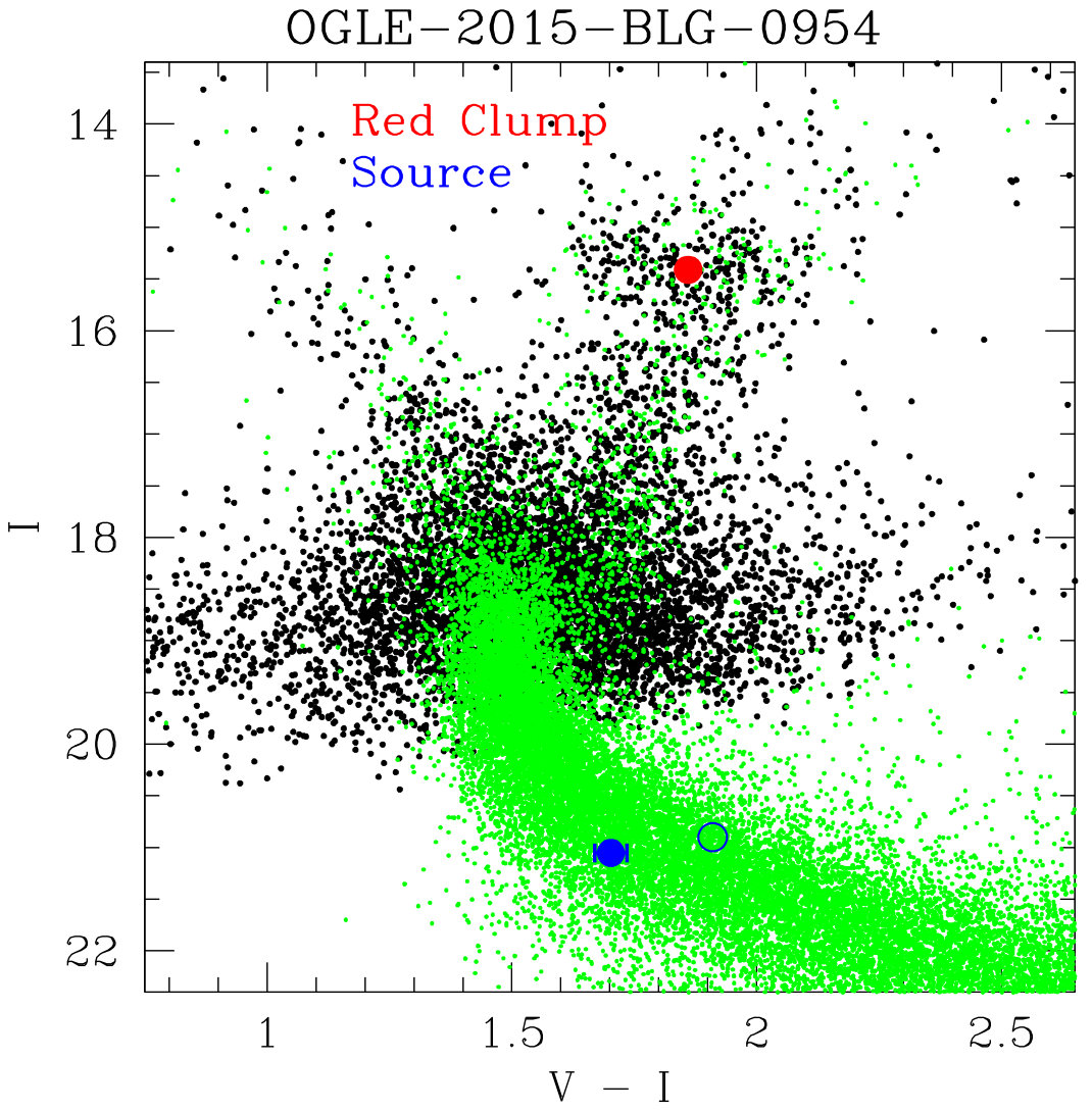 Figure 1
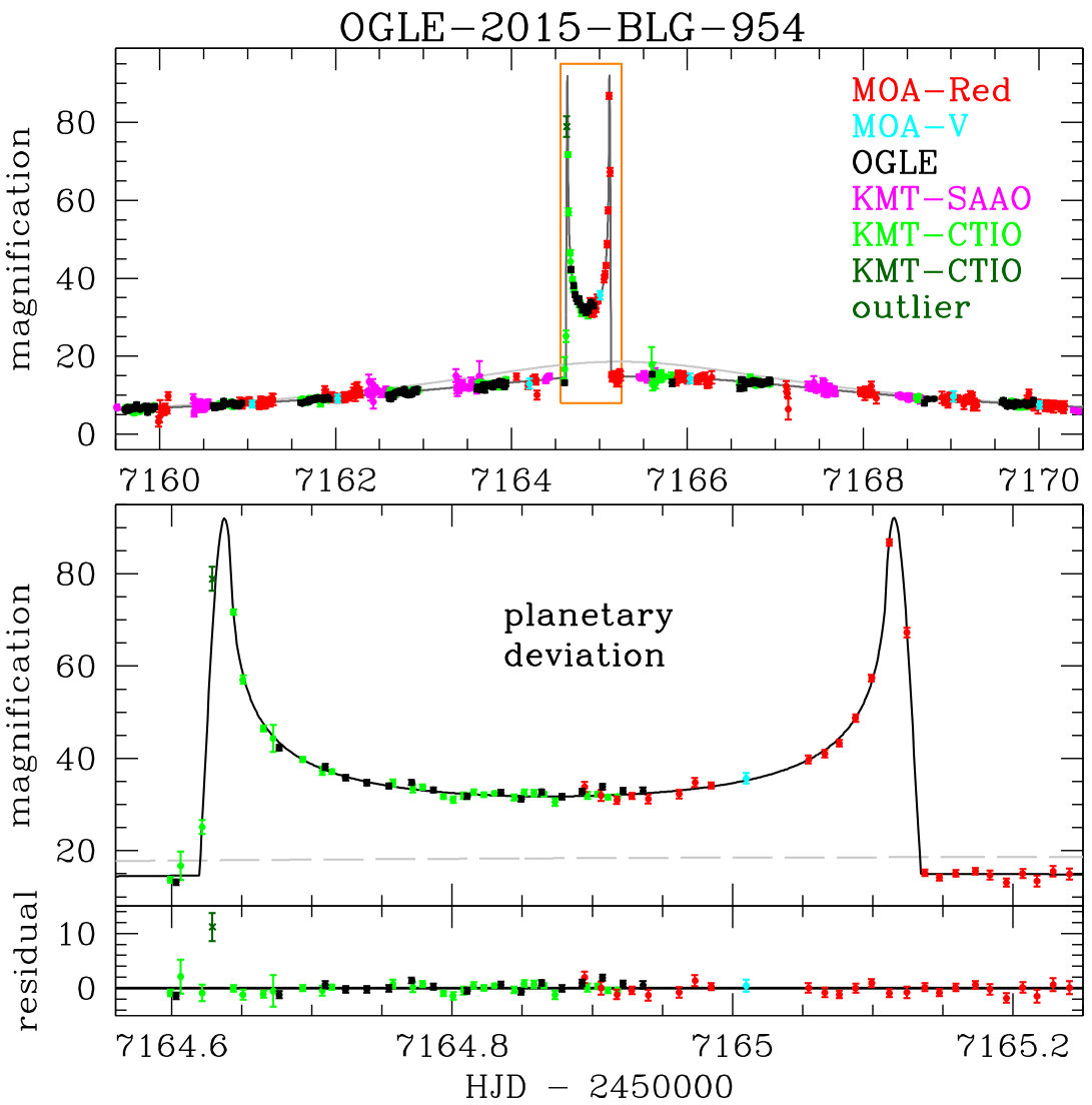 Figure 2
| MCMC averages | |||||
|---|---|---|---|---|---|
| parameter | units | ||||
| days | 39.603 | 39.386 | 39.5(1.2) | 39.4(1.2) | |
| 7165.2277 | 7165.1763 | 7165.227(9) | 7165.176(8) | ||
| 0.053803 | 0.047302 | 0.0541(20) | 0.0473(17) | ||
| 0.79750 | 1.35247 | 0.7977(32) | 1.3529(30) | ||
| radians | 1.40353 | 1.40857 | 1.4039(41) | 1.4085(39) | |
| 0.01031 | 0.01134 | 0.01035(26) | 0.01136(31) | ||
| days | 0.01153 | 0.01148 | 0.01152(28) | 0.01144(29) | |
| 21.053 | 21.038 | 21.047(33) | 21.037(32) | ||
| 1.702 | 1.702 | 1.702(31) | 1.702(31) | ||
| fit | 16820.62 | 16821.20 | |||
| Parameter | units | value | 2- range |
|---|---|---|---|
| kpc | 0.4-3.0 | ||
| 0.09-0.83 | |||
| 1.0-9.3 | |||
| AU | 0.5-4.5 | ||
| AU | 0.6-9.3 | ||
| mas/yr | 10.3-13.3 | ||
| mas | 1.12-1.44 | ||
| mag | 18.55-21.78 | ||
| mag | 16.27-18.12 |
Peer Reviews
No public reviews on file for this paper yet. If you reviewed it on a platform where reviews are public (OpenReview, ICLR, NeurIPS, ICML), you can paste yours below so the community can read it here.
Videos
No videos yet. Explain this paper in a talk, walkthrough, or lecture? Add one.
MOA Data Reveal a New Mass, Distance, and Relative Proper Motion for Planetary System
OGLE-2015-BLG-0954L
D.P. Bennett11affiliationmark: 22affiliationmark: , I.A. Bond33affiliationmark: ,
and
F. Abe4, Y. Asakura4, R. Barry1, A. Bhattacharya11affiliationmark: 22affiliationmark: , M. Donachie5, P. Evans5, A. Fukui6, Y. Hirao7, Y. Itow4, N. Koshimoto7, M.C.A. Li5, C.H. Ling3, K. Masuda4, Y. Matsubara4, Y. Muraki4, M. Nagakane7, K. Ohnishi8, C. Ranc1, N.J. Rattenbury5, To. Saito9, A. Sharan5, D.J. Sullivan10, T. Sumi7, D. Suzuki1,11, P.J. Tristram12, T. Yamada13, T. Yamada7, and A. Yonehara13
(The MOA Collaboration)
1Code 667, NASA Goddard Space Flight Center, Greenbelt, MD 20771, USA;
Email: [email protected]
2Deptartment of Physics, University of Notre Dame, Notre Dame, IN 46556, USA;
3Institute of Natural and Mathematical Sciences, Massey University, Auckland 0745, New Zealand
4Institute for Space-Earth Environmental Research, Nagoya University, Nagoya 464-8601, Japan
5Department of Physics, University of Auckland, Private Bag 92019, Auckland, New Zealand
6Okayama Astrophysical Observatory, National Astronomical Observatory of Japan, 3037-5 Honjo, Kamogata, Asakuchi, Okayama 719-0232, Japan
7Department of Earth and Space Science, Graduate School of Science, Osaka University, Toyonaka, Osaka 560-0043, Japan
8Nagano National College of Technology, Nagano 381-8550, Japan
9Tokyo Metropolitan College of Aeronautics, Tokyo 116-8523, Japan
10School of Chemical and Physical Sciences, Victoria University, Wellington, New Zealand
11Institute of Space and Astronautical Science, Japan Aerospace Exploration Agency, Kanagawa 252-5210, Japan
12University of Canterbury Mt. John Observatory, P.O. Box 56, Lake Tekapo 8770, New Zealand
13Department of Physics, Faculty of Science, Kyoto Sangyo University, 603-8555 Kyoto, Japan
Abstract
We present the MOA Collaboration light curve data for planetary microlensing event OGLE-2015-BLG-0954, which was previously announced in a paper by the KMTNet and OGLE Collaborations. The MOA data cover the caustic exit, which was not covered by the KMTNet or OGLE data, and they provide a more reliable measurement of the finite source effect. The MOA data also provide a new source color measurement that reveals a lens-source relative proper motion of mas/yr, which compares to the value of mas/yr reported in the KMTNet-OGLE paper. This new MOA value for has an a priori probability that is a factor of \lower 2.15277pt\hbox{;\buildrel>\over{\sim};}100 times larger than the previous value, and it does not require a lens system distance of kpc. Based on the corrected source color, we find that the lens system consists of a planet of mass orbiting a star at an orbital separation of AU and a distance of kpc.
gravitational lensing: micro, planetary systems
1 Introduction
Gravitational microlensing has a unique niche among methods for studying exoplanet systems (Bennett, 2008; Gaudi, 2012) because of its sensitivity to planets extending down to low masses (Bennett & Rhie, 1996) beyond the snow line (Mao & Paczyński, 1991; Gould & Loeb, 1992), where planet formation is thought to be the most efficient (Ida & Lin, 2005; Lecar, 2006; Kennedy et al., 2006; Kennedy & Kenyon, 2008; Thommes et al., 2008), according to the leading core accretion planet formation theory (Lissauer, 1993; Pollack et al., 1996). Statistical analyses of exoplanetary microlensing samples have indicated that planets with roughly Neptune masses are more common than Jupiters (Sumi et al., 2010; Gould et al., 2010; Cassan et al., 2012; Shvartzvald et al., 2016), and the recent analysis of a larger sample by the MOA Collaboration (Suzuki et al., 2016) has indicated a break and likely peak in the exoplanet mass ratio function at a mass ratio of . This is broadly consistent with the predictions of the core accretion theory (Laughlin et al., 2004).
Thus far, the statistical analyses of the exoplanets found by microlensing have focused on the planetary parameters that are most easily measured in microlensing events, the mass ratio, , and the separation, , in Einstein radius units. Fortunately, it is possible to measure additional parameters that can constrain the lens system mass, , and distance by making use of the following equations,
[TABLE]
where and and the lens and source distances, is the angular Einstein radius, and is the microlensing parallax (Gould, 1992; Alcock et al., 1995). For most planetary microlensing events, can be directly determined from finite source effects, which provides a measurement of the source radius crossing time, . When is known, then is determined from the expression , where is the Einstein radius crossing time and is the angular source size. Both and are normally determined from the model of the microlensing light curve, but generally requires a measurement of both the source brightness and color (Kervella et al., 2004; Boyajian et al., 2014). Measurement of and also yield the lens-source relative proper motion, , which can sometimes be used to constrain the lens mass and distance based on kinematic arguments that employ models of the stellar population of the Milky Way.
The source radius crossing time is determined for most planetary microlensing events, so that we can determine and use the first expression of equation 1 to constrain the lens mass and distance. For a subset of events, can be measured due to the orbital motion of the Earth (Gaudi et al., 2008; Bennett et al., 2010, 2008; Muraki et al., 2011) or observations from a satellite in a Heliocentric orbit (Street et al., 2016). When combined with a measurement of , this gives the direct measurement of the lens mass given by the last expression of equation 1. The lens mass can also be determined with a combination of a measurement and a measurement of the host star brightness in one or more passbands (Bennett et al., 2006, 2007, 2015; Batista et al., 2015; Fukui et al., 2015; Skowron et al., 2015). Alternatively, for events without measurements, it is possible to determine the lens mass by combining measurements of and the host star brightness (Koshimoto et al., 2017b). For complicated systems, like the OGLE-2007-BLG-349L circumbinary planetary system (Bennett et al., 2016), it is necessary to measure , , and the lens system brightness to resolve all the degeneracies in the interpretation. However, for simpler systems, the measurements of , , and the lens brightness provides redundancy that confirms that these methods are giving reliable results (Gaudi et al., 2008; Bennett et al., 2010; Beaulieu et al., 2016).
The next step in the statistical analysis of wide orbit sample exoplanetary microlens systems will be to include the constraints from measurements of , , and the host star brightness for large statistical samples, such as that of Suzuki et al. (2016). This will enable us to expand our analysis beyond the mass ratio and separation in Einstein radius units to determine the exoplanet mass function as a function of the host star mass, as well as a function of Galactocentric distance. This analysis will include not only those planetary systems with a full determination of their mass and distance, but also events with only a measurement of a single additional parameter, either or . These partial constraints can be useful in a Bayesian statistical analysis.
If we are going to include these additional constraints in statistical analyses of exoplanet properties, it is important to ensure that the measurements used are largely free of systematic errors. This is relatively straight forward to avoid mistakes in finding the basic microlensing parameters (Gould et al., 2013). There has been one recent modeling mistake (Udalski et al., 2015a; Han et al., 2016), but in fact, this was essentially identical to a much earlier modeling error (Bennett et al., 1999; Albrow et al., 2000; Jung et al., 2013) and not a sign of a fundamental problem with modeling methods. However, these basic modeling errors are not the only errors that concern us. Recent analyses have shown that it is quite possible to mistakenly attribute excess flux seen in the vicinity of the microlensed source star to the lens star. Koshimoto et al. (2017a) have used a Bayesian analysis to show that it is often possible for excess flux from binary companions to the lens or source stars or even ambient stars to be confused for the flux of the lens stars, although this effect is much smaller if stars have a much higher planet hosting probability than low-mass stars. Bhattacharya et al. (2017) have recently shown that the excess flux detected for the planetary microlensing event MOA-2008-BLG-310 (Janczak et al., 2010) does not have a relative proper motion consistent with the lens star. Most likely, the flux is due to an ambient star, unrelated to the microlensing event. In contrast, the excess flux seen in 4 passbands () for planetary microlensing event OGLE-2005-BLG-169 has been confirmed to have the value predicted by the microlensing light curve (Bennett et al., 2015; Batista et al., 2015).
There is statistical evidence of errors in the lens distance estimates for 31 published exoplanets. Penny et al. (2016) find an excess of planetary lens systems located close to the position of the Sun, with D_{L}\lower 2.15277pt\hbox{;\buildrel<\over{\sim};}1\,kpc. This excess is likely to be due to errors in measurement of or , as errors in both parameters tend to produce events with anomalously close distances. Microlensing parallax, , is quite difficult to measure for distant lenses, particularly those that reside in the Galactic bulge. So, a problem with the light curve photometry or modeling might result in a spuriously large value, which would imply a nearby lens. In fact, this is what happened with OGLE-2013-BLG-0723. The original model (Udalski et al., 2015a), which included a planet, had an anomalously large value. However, the paper describing the correct, planet-free model for this event (Han et al., 2016) shows that this anomalously large is the result of the incorrect model trying to account for a feature that the model cannot fully explain. MOA-2010-BLG-328 (Furusawa et al., 2013) is another example of an event with a suspiciously large value, although in this case the authors recognized the issue and considered the possibility that the signal could be false, a case of source orbital motion (referred to as xallarap). Another possible example is MOA-2007-BLG-192, which was published as possible brown dwarf plus planet event, with a planet of only a few Earth masses (Bennett et al., 2008). A analysis of adaptive optics (AO) follow-up data (Kubas et al., 2012) indicated the apparent detection of the host star near the bottom of the main sequence, but this analysis did not include a detailed analysis of the possibility that the excess flux may not be due to the lens tar.
MOA-2014-BLG-262 is the event with the situation most similar to the event that we discuss in this paper (Bennett et al., 2014). This was a relatively short duration event with a clear signal of a planetary mass ratio companion, but the best fit model implied a very large relative proper motion, mas/yr. This seemed to imply that the lens must be nearby, but the short event duration implied a small value. From equation 1, this implies a low mass host of only a few Jupiter masses if the host is as close as the large relative proper motion would suggest. So, this would imply an apparently isolated planet with a planetary mass ratio moon. However, a more careful analysis revealed another model with a value that was only slightly larger than the best fit, but with a larger value. This implied a significantly lower relative proper motion of mas/yr, which is consistent with a lens in the Galactic bulge. In fact, because of the small value for this event, a bulge lens is favored.
In this paper, we consider planetary microlensing event OGLE-2015-BLG-0954. The planetary signal was seen data both the data taken from Chile by the Optical Gravitational Lensing Experiment (OGLE) and Korean Microlensing Telescope Network (KMTNet). They show that their data can only be explained by a relatively high mass ratio planet with an unusually large relative proper motion of mas/yr by Shin et al. (2016), hereafter S16. Since the lower proper motion solution for MOA-2014-BLG-262 is strongly favored by its prior probability, this would be the highest relative proper motion ever seen for a planetary microlensing event, although a non-planetary event has an even higher relative proper motion (Gould et al., 2009). S16 conclude that the lens must be located close to us, as a distance of kpc.
Because of an error with the MOA alert system, MOA did not issue an alert on this event, but in fact, MOA had good coverage of this event, including coverage of the caustic exit in good observing conditions. This feature was not observed by OGLE or KMTNet. We model this event with MOA data in addition to the OGLE and KMTNet data, and we find results consistent with those of S16, except for the source color. We find a bluer source, which implies a smaller source radius, and .
This paper is organized as follows. In Section 2 we describe the published light curve data, as well as new MOA data and its photometry. In Section 3, we describe our light curve modeling. We describe the photometric calibration and the determination of the primary source star radius in Section 4, and then we derive the lens system properties in Section 5. Our conclusions are presented in Section 6.
2 Light Curve Data and Photometry
The microlensing event OGLE-2015-BLG-0954 at :00:44.24, :39:39.2, and Galactic coordinates , was discovered by the OGLE collaboration (Udalski et al., 2015b) Early Warning System (EWS) (Udalski et al., 1994), and the OGLE and KMTNet photometry was presented in the KMTNet-led discovery paper (S16). The observing cadence for both OGLE and KMTNet telescope at the Cerro Tololo Inter-American Observatory (CTIO) would normally be minutes and minutes, respectively. However, the weather at the time of the planetary caustic entrance was reportedly “unstable” at CTIO and was probably poor at the OGLE telescope at the Las Campanas Observatory (LCO), as well. As a result, the OGLE data does not cover the caustic crossing. The KMT-CTIO coverage was better, but some of the critical data was taken in poor observing conditions. This is probably the reason that the KMT-CTIO observation near the top of the caustic crossing is a - outlier as indicated in Figure 1.
The MOA Collaboration did not identify this event with its alert system, but we found a strong signal including coverage of the caustic exit, indicating that the event was missed due to an alert system (Bond et al., 2001) error, probably an oversight by the observer. We obtained optimized photometry via a reduction of and images obtained by extracting sub-images centered on the event (Bond et al., 2017). For this analysis, we used observations from April, 2012 through August, 2016. We used our own difference imaging implementation that incorporates a numerical kernel as described by (Bramich, 2008) with our own modification to allow for a spatial variation of the kernel across the field-of-view in a similar manner to that given by (Alard, 2000). The photometry for both the reference and difference images were measured using an analytic PSF model of the form used in the DoPHOT photometry code (Schechter, Mateo, & Saha, 1993). Trends in the photometry with seeing, airmass, and differential refraction (parameterized by the hour angle and airmass) were removed based on the observed trends in 2012-2014 and 2016. The MOA photometry consists of 252 observations in the passband and 9663 after removing 7 4- outliers from the best fit model, which were all separated by more than a week from the planetary signal. The MOA instrumental magnitudes were calibrated by cross referencing stars in the DoPHOT catalog to stars in the OGLE-III catalog which provides measurements in the standard Kron-Cousins and Johnson passbands (Szymański et al., 2011). This allows us to derive relations to calibrate the MOA photometry to standard magnitudes.
We obtained the KMTNet and OGLE -band light curve data from KMTNet group, and we used all of the OGLE and KMT-SAAO data that was provided. The KMT-CTIO data consisted of 3 separate light curves due to changes in the camera electronics. (This was the first year of the KMTNet survey.) Since the long term behavior of the light curve is well covered by MOA and OGLE, we include only the second portion of the KMT-CTIO light curve, which consists of 1187 observations. However, the data point closest to the peak of the light curve is a 4- outlier, so we do not include that data point in our modeling.
3 Light Curve Models
Our light curve modeling was done using the image centered ray-shooting method (Bennett & Rhie, 1996), and we employed the initial condition grid search method outlined in Bennett (2010) to search the binary lens parameter space for solutions. Unsurprisingly, we recovered solutions very similar to those presented in S16. The parameters of our best fit close and wide models are shown in Table 1, along with the Markov Chain Monte Carlo (MCMC) results for solutions centered on each best fit model. The model parameters that also apply to a single lens system are the Einstein radius crossing time, , and the time, , and distance, , of closest approach between the lens center-of-mass and the source star. Binary lens models also include the mass ratio of the secondary to the primary lens, , the angle between the lens axis and the source trajectory, , and the separation between the lens masses, . Figure 1 shows the light curve and best fit close model, which is slightly favored over the best fit wide model. The length parameters, and , are normalized by the Einstein radius of this total system mass, , where and and are the lens and source distances, respectively. ( and are the Gravitational constant and speed of light, as usual.)
For every passband, there are two parameters to describe the unlensed source brightness and the combined brightness of any unlensed “blend” stars that are superimposed on the source. Such “’blend” stars are quite common because there are usually several relatively bright, main sequence stars in each seeing disk. These stars generally are not microlensed because this requires lens-source alignment of \lower 2.15277pt\hbox{;\buildrel<\over{\sim};}\theta_{E}\sim 1\,mas. The source and blend fluxes are treated differently from the other parameter because the observed brightness has a linear dependence on them, so for each set of nonlinear parameters, we can find the source and blend fluxes that minimize the exactly, using standard linear algebra methods (Rhie et al., 1999).
The source radius crossing time, , is an important parameter because the both and depend on it. Because of KMTNet data had a 4- photometric outlier on the one caustic crossing resolved in the discovery paper (S16), we had expected a high probability that our best fit values would differ from the S16 values. However, our values are and days for the close and wide models, respectively. These compare to the S16 values of and days for the close and wide models, so our values are larger by only about 1-. Thus, our new values will not reduce the value reported by S16 by a significant amount.
4 Photometric Calibration and Source Radius
The measurement of the angular source radius, , can have a significant effect the lens-source relative proper motion measurement. This requires the determination of the extinction corrected source brightness and color. The first step is to convert our instrumental and magnitudes to calibrated OGLE-III magnitudes (Szymański et al., 2011). Using the photometry described in Section 2, we derive
[TABLE]
where we have used comparison stars with to derive the transformation. Although the MOA-red filter is roughly equivalent to Cousins plus Cousins , the high extinction of the bulge fields reduces the bluer flux and pushes the to be closer to Cousins rather than Cousins .
The next step is to determine the extinction. Figure 2 shows the color magnitude diagram (CMD) of the stars in the OGLE-III catalog within of OGLE-2016-BLG-0954 along with the Baade’s Window HST CMD (Holtzman et al., 1998) (in green) shifted to the extinction and bulge distance for the position of our target. We determine the red clump centroid to be located at , , whereas Nataf et al. (2013) predict the unextincted red clump centroid to be located at , at this Galactic longitude. This implies and -band extinctions of and . From Table 1, we see that the best fit source magnitude and color are and , so that the unextincted source magnitude and color are and . We determine the angular source radius using
[TABLE]
which comes from the Boyajian et al. (2014) analysis using a restricted set of data using only stars with (Boyajian, private communication, 2014). This gives as for the best fit model, which is a factor of 1.49 smaller than the S16 value of . This difference is due to the fact that we find the source 0.14 mag fainter and 0.28 mag redder than the values published by S16, as indicated by the open blue circle in Figure 2. Because the coefficient of the term in Equation 4 is a little more than twice as large as the coefficient of the term, we can see that % of this difference is due to the difference in color measurements, while the remaining % is due to our slightly larger value and fainter source.
This new implies an angular Einstein radius of , where the error bar includes only the contribution from the uncertainty. (The contribution from the model parameter uncertainties will be presented in Section 5.) This value is a factor of 1.46 smaller than the S16 value, but it is still much larger than average. From Equation 1, we can see that it implies a mass of for a source at kpc and a lens at kpc. However, the OGLE and MOA data are not compatible with a main sequence star any more massive than main sequence star at kpc at the position of the source (as we discuss below in Section 5).
4.1 Comparison of Source Color Measurements
Since there are many more measurements than measurements, the uncertainty in the color measurement is determined by the uncertainty of the source brightness in the band. Most of the magnified data responsible for our band measurements is shown Figure 1 as the cyan colored points. There is one observation per day in the relatively good observing conditions near the peak of this event. There are 7 data points with magnification , and these points have a total . This corresponds to a if we assume that these 7 data points control both the source and blend brightness parameters for the band. This small value is correlated with relatively small photometric error bars on these data points, which implies that the band data near the light curve peak should be reliable. There are many data points at low magnification, so we expect that neither the high magnification points nor the low magnification points should be affected by systematic errors due to photometric irregularities.
It is more difficult to investigate potential photometric problems with the OGLE and KMT-CTIO -band data, because we do not have access to the data. The OGLE -band data have similar scatter to data interior to the caustic crossing, but S16 report . Since this error bar is 2.3 times larger than the derived from the MOA data, it seems unlikely that OGLE has any -band observations interior to the caustic crossing.
The situation is different for the KMT-CTIO data, as S16 report that one out of every 6 images are taken in the -band by this telescope. Since the KMT-CTIO -band data set contains 27 data points above magnification 30 on the night of the caustic entry, we might expect that they also have -band at magnification . However, S16 report a KMT-CTIO color estimate of , so the error bar is also larger than the derived from the MOA data, despite the likelihood of many more -band observations than MOA. While we cannot be certain of the situation with the KMT-CTIO -band data, there are several causes for concern. First, the light curve data were reduced with DoPHOT instead of difference imaging. This is often adequate for bright sources in good observing conditions, but this event was quite faint, except for the night of the caustic crossing when weather conditions at CTIO were reportedly unstable.
Second, the color is not determined by a fit to the light curve. Instead, it is determined by a linear fit to and -band observations that are approximately simultaneous. This is a common method used when there is some uncertainty about the correct model. However, it is subject to large systematic errors if the magnification changes significantly during the time interval that is considered “approximately simultaneous.” S16 use the criteria that two observations can be consider simultaneous if they are separated by days, which is the interval between the tick marks in the lower two panels of Figure 1. This is a poor assumption for the night of the caustic entry. According to the best fit model, the event brightens by a factor of in the , and then drops by factors of 1.51, 1.13, and 1.055 over the intervals , , and , respectively. It is only after that the light curve variation over this 0.05 interval drops below the quoted 0.05 mag uncertainty of the color measurement, but two thirds of the KMT-CTIO observations were taken before on the night of the caustic crossing. For these reasons, we do not use the KMT-CTIO color estimate in our calculations.
We also have the option of using the OGLE color of , which is at most, marginally inconsistent with the MOA color. The weighted combination of these measurements is . This is only 1.1- above the MOA value of , so the inclusion of the OGLE measurement would have little effect on our conclusions.
The Bayesian analysis presented in the next section can also be used to compare the a priori probabilities for the MOA and KMTNet-OGLE values. This analysis indicates that mas/yr is 111 times more likely than mas/yr. Because both cases favor nearby lenses, these analyses are not dependent on the detailed structure of the Galactic bulge model, but they do depend on the high velocity tails of the velocity distribution for all the stellar components of the Galaxy, which our method is optimized for (Bennett et al., 2014).
5 Lens System Properties
Because we are lacking a microlensing parallax measurement and a lens brightness measurement, we are unable to use the expressions in Equation 1 to directly determine the lens mass and distance. Instead, we are limited to a Bayesian analysis using the mass-distance relation in Equation 1. This is similar to the situation for event MOA-2011-BLG-262 (Bennett et al., 2014) because the value is larger than for most microlensing events, so we use the Galactic model employed for the Bennett et al. (2014) analysis because it was designed to include the high velocity components of the galaxy, such as the thick disk and the spheroid (or stellar halo), while also enforcing the Galactic escape velocity as an upper limit on the velocities. The large value does favor nearby lenses, but for the MOA-2011-BLG-262 event, with a slightly larger , a lens location in the Galactic bulge received comparable probability to nearby lens locations. The situation for OGLE-2015-BLG-0954 is different because of its much larger and values. The mass-distance relation from Equation 1 implies that a bulge lens would have to be faint but also very massive. So, it could only be a stellar mass black hole. We do not consider black hole hosts in our analysis, but if we did, the probability of such a lens system would still be small because stellar mass black holes are known to be rare compared to main sequence stars even though their occurrence rate is not very well known.
The results or our Bayesian analysis are given in Table 2. The main difference with the S16 results is that the lens system is likely to be at a larger distance of kpc, compared to claimed by S16. (This is derived from their equation 14.) With our smaller and values, we find that this event is consistent with a large range of host star and planet masses. This new distance reduces the tension seen by Penny et al. (2016) in the number of planet discoveries estimated to be at small distances, kpc. Our 68% and 95% for the host mass are 0.16- and 0.09-, respectively. The 2- upper limit on the host mass is due to the observed upper limit on the host star flux (assuming a main sequence host star). S16 reported 2 different mass values: an upper limit of for a main sequence host and for a host of any type. These are an artifact of their apparent color measurement error, and the true range of host masses is much larger. This larger range of host masses implies a large range of planet masses with 68% and 95% confidence level ranges of 1.8- and 0.9-. The ranges of three-dimensional separations predicted for this event are 1.1-AU and 0.6-AU at the 68% and 95% confidence levels.
The and band brightness ranges for the lens (and host) star are also given in Table 2. The 95% confidence level ranges are and , which compare to the measured source brightness (from Table 1) of . This implies that the lens star will be somewhere between one half and and ten times as bright as the source in the -band, with a smaller range of brightness in the -band. The HST analysis of (Bhattacharya et al., 2017) implies that the lens-source separation can already be measured with HST images, while the two stars should be resolvable with Keck AO images by 2020 (Batista et al., 2015). The measurement of the host star brightness will allow the host mass to be determined through the combination of the mass distance relation (equation 1) and a mass-luminosity relation (Bennett et al., 2006).
6 Discussion and Conclusions
At present, all the statistical analyses of the properties of planetary systems found by microlensing (Sumi et al., 2010; Gould et al., 2010; Cassan et al., 2012; Shvartzvald et al., 2016; Suzuki et al., 2016) have characterized the distribution with the mass ratio, , and projected separation, , of the discovered planets, although Suzuki et al. (2016) did also look at the dependence. However, we now have a growing number of measurements off additional parameters that can be used to learn more details of the exoplanet properties beyond the snow line. For a growing number of events, we can determine masses from microlensing parallax measurements, either from the orbital motion of the Earth (Gaudi et al., 2008; Bennett et al., 2008, 2016; Muraki et al., 2011; Han et al., 2013; Furusawa et al., 2013; Skowron et al., 2015; Sumi et al., 2016; Koshimoto et al., 2017b) or from observations from a satellite in a Heliocentric orbit (Street et al., 2016). High angular resolution follow-up observations can allow the determination of the planet and host star masses using the mass-distance relation given in equation 1 and a mass-luminosity relation (Bennett et al., 2006, 2015; Batista et al., 2015; Dong et al., 2009; Fukui et al., 2015; Beaulieu et al., 2016). The combined results of these , , and host star brightness measurements will be to allow us to expand our statistical analysis beyond the simple mass ratio and separation measurements to include dependence of exoplanet properties on the host star mass and Galactocentric distance. So, microlensing had the potential to give us a comprehensive picture of planets that orbit beyond the snow line throughout the Galaxy.
In order to realize the potential of these additional measurements, it is important to ensure that these additional measurements are free of errors. Penny et al. (2016) noted a statistical indication of such errors in the large number of published planetary microlensing events with lens distances of kpc and especially kpc. The error that yielded one of these events has already been found (Udalski et al., 2015a; Han et al., 2016), as a large spurious parallax signal resulted from using the wrong lens model geometry. A different type of difficulty has been identified by Bhattacharya et al. (2017) and Koshimoto et al. (2017a). They have identified cases where excess flux on top of the source star could be mistakenly attributed to the lens star. The solution to this difficulty is to ensure that the lens-source relative proper motion matches the model prediction (Bennett et al., 2015; Batista et al., 2015).
The problem that we have identified with the S16 analysis of OGLE-2015-BLG-0954 is a problem with the source color measurement. We have not seen the -band data used for the S16 paper, so we can not be sure why our results disagree with theirs. However, the difference imaging method (Tomaney & Crotts, 1996; Alard & Lupton, 1998) has been the state-of-the-art crowded field photometry method for microlensing surveys for nearly two decades (Alcock et al., 1999; Udalski, 2003). For some difference imaging implementations, it has been difficult to put the light curve photometry on the same photometric scale as the photometry of the stars in the reference frame because different PSF models are used in each case. However, the OGLE Collaboration solved this problem with its pipeline back in 2003 (Udalski, 2003). Bennett et al. (2012) showed that it is straight forward to modify a DoPHOT-like (Schechter, Mateo, & Saha, 1993) code to produce photometry of difference images on the same photometry scale as the DoPHOT reference frame photometry, and the MOA collaboration has developed the code used in this paper for this task (Bond et al., 2017). We recommend that difference imaging photometry should always be used for color measurements in the future.
The implied properties of the OGLE-2015-BLG-0954Lb planet are not greatly effected by the change in the and values. The previous, relatively tight, limits on the mass of the host star and planet are now substantially weakened. The host star is no longer limited to be a low mass star with , and instead is in the range (at 95% confidence). Fortunately, if the lens is a main sequence star, it should be easily detectable with HST or AO observations.
D.P.B., A.B., D.S. and C.R. were supported by NASA through grants NASA-NNX13AF64G and NNX16AN59G. Work by C.R. was also supported by an appointment to the NASA Postdoctoral Program at the Goddard Space Flight Center, administered by USRA through a contract with NASA. The MOA project in Japan is supported by JSPS KAKENHI grants JSPS24253004, JSPS26247023, JSPS23340064, JSPS15H00781, JP16H06287, and JP17H02871.
The reference list from the paper itself. Each links out to its DOI / PubMed record.
- 1Alard (2000) Alard, C. 2000, A&AS, 144, 363
- 2Alard & Lupton (1998) Alard, C. & Lupton, R.H. 1998, Ap J, 503, 325
- 3Albrow et al. (2000) Albrow, M.D. 2000, Ap J, 534, 894
- 4Alcock et al. (1995) Alcock, C., Allsman, R. A., Alves, D., et al. 1995, Ap J, 454, L 125
- 5Alcock et al. (1999) Alcock, C., Allsman, R. A., Alves, D., et al. 1999, Ap J, 521, 602
- 6Batista et al. (2015) Batista, V., Beaulieu, J.-P., Bennett, D.P., et al. 2015, Ap J, 808, 170
- 7Beaulieu et al. (2016) Beaulieu, J.-P., Bennett, D. P., Batista, V., et al. 2016, Ap J, 824, 83
- 8Bennett (2008) Bennett, D.P, 2008, in Exoplanets, Edited by John Mason. Berlin: Springer. ISBN: 978-3-540-74007-0, (ar Xiv:0902.1761)