TL;DR
This paper introduces autoscaling Bloom filters, a flexible data structure that dynamically balances true positives and false positives by adjusting its capacity, supported by mathematical analysis and a minimization procedure.
Contribution
It proposes a novel autoscaling Bloom filter that generalizes counting Bloom filters with adjustable capacity and probabilistic bounds, enhancing control over false positives.
Findings
Mathematical analysis of autoscaling Bloom filter performance
Procedure for minimizing false positive rate
Demonstrated adjustable capacity with probabilistic guarantees
Abstract
A Bloom filter is a simple data structure supporting membership queries on a set. The standard Bloom filter does not support the delete operation, therefore, many applications use a counting Bloom filter to enable deletion. This paper proposes a generalization of the counting Bloom filter approach, called "autoscaling Bloom filters", which allows adjustment of its capacity with probabilistic bounds on false positives and true positives. In essence, the autoscaling Bloom filter is a binarized counting Bloom filter with an adjustable binarization threshold. We present the mathematical analysis of the performance as well as give a procedure for minimization of the false positive rate.
Click any figure to enlarge with its caption.
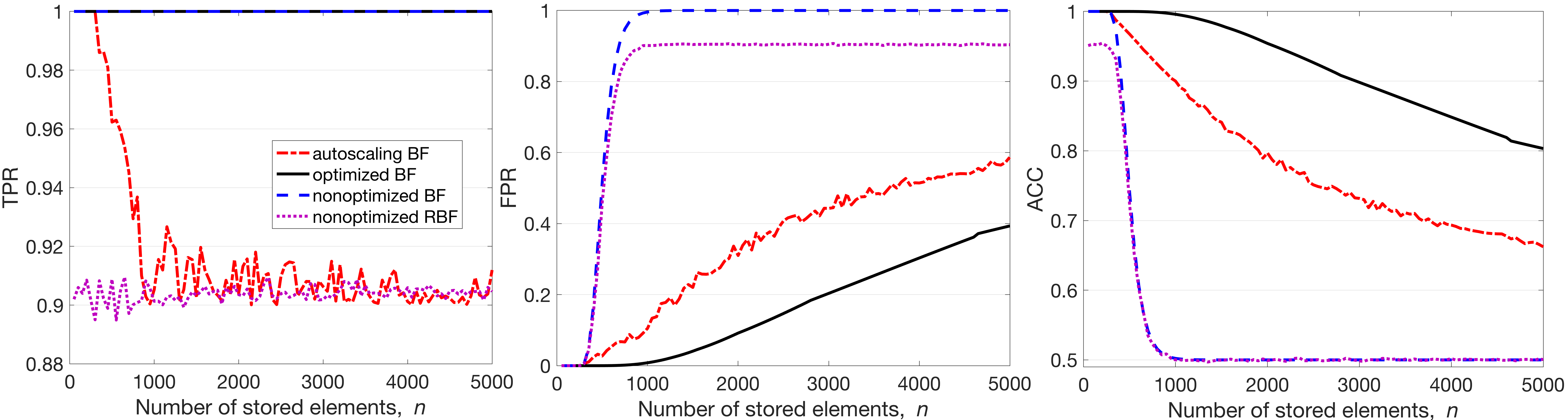 Figure 1
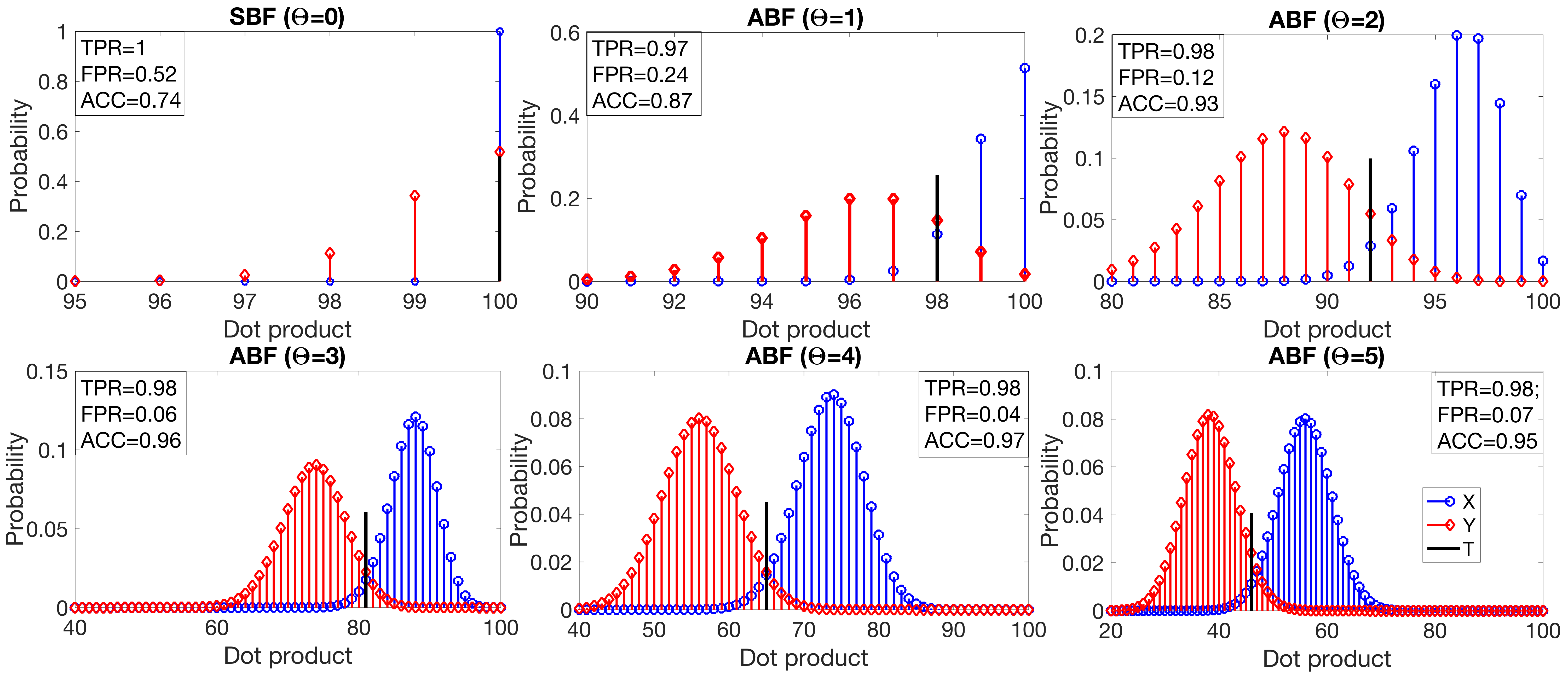 Figure 2
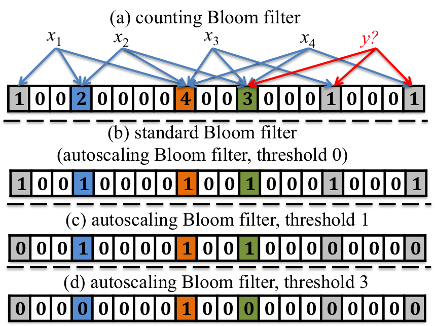 Figure 3
Peer Reviews
No public reviews on file for this paper yet. If you reviewed it on a platform where reviews are public (OpenReview, ICLR, NeurIPS, ICML), you can paste yours below so the community can read it here.
Code & Models
Videos
No videos yet. Explain this paper in a talk, walkthrough, or lecture? Add one.
11institutetext: 1 Luleå University of Technology, Luleå, Sweden.
11email: {denis.kleyko, evgeny.osipov}@ltu.se
2ETH Zurich, Zurich, Switzerland.
11email: [email protected]
3Independent Researcher, Melbourne, Australia.
11email: [email protected]
Autoscaling Bloom Filter
Controlling Trade-off Between True and False Positives
Denis Kleyko 11
Abbas Rahimi 22
Ross W. Gayler 33
Evgeny Osipov 11
Abstract
A Bloom filter is a simple data structure supporting membership queries on a set. The standard Bloom filter does not support the delete operation, therefore, many applications use a counting Bloom filter to enable deletion. This paper proposes a generalization of the counting Bloom filter approach, called “autoscaling Bloom filters”, which allows adjustment of its capacity with probabilistic bounds on false positives and true positives. In essence, the autoscaling Bloom filter is a binarized counting Bloom filter with an adjustable binarization threshold. We present the mathematical analysis of the performance as well as give a procedure for minimization of the false positive rate.
Keywords:
B
loom filter, counting Bloom filter, autoscaling Bloom Filter, true positive rate, false positive rate.
1 Introduction
Many applications require fast and memory efficient querying of an item’s membership in a set. A Bloom filter (BF) is a simple binary data structure, which supports approximate set membership queries.
The standard BF (SBF) allows adding new elements to the filter and is characterized by a perfect true positive rate (i.e. 1), but nonzero false positive rate. The false positive rate depends on the number of elements to be stored in the filter and on the filter’s parameters, including the number of hash functions and the size of the filter. However, SBF lacks the functionality of deleting an element. Therefore, a counting Bloom filter (CBF) [1], providing the delete operation, is commonly used. When the size of the CBF and the number of elements to be stored are known, the number of hash functions can be optimized to minimize the false positive rate.
Another practical issue is that the parameters of a BF (size of filter and number of hash functions) can not be altered once it is constructed. If the current filter does not satisfy the performance requirements (e.g. false positive rate) it is necessary to rebuild the entire filter, which is computationally expensive. Therefore, the optimization of a BF is problematic and costly when the number of elements to be stored is unknown or varies dynamically.
To address the issue of optimizing BF performance without rebuilding the filter, we propose the autoscaling Bloom filter (ABF), which is derived from a CBF and allows minimization of the false positive rate in response to changes in the number of stored elements without requiring rebuilding of the entire filter. The reduction in false positive rate is achieved by optimizing a threshold parameter used to derive the ABF from the CBF. ABF operates with fixed resources (i.e. fixed size storage array and fixed hash functions) for a wide dynamic range of number of input elements to be stored. The trade-off made by ABF for this flexibility is a slight reduction of the true positive rate (which is always 1 in CBF). It is important to note that a less than perfect true positive rate can be tolerated in many applications including networking [2], and generally in the area of approximate computing where errors and approximations are acceptable as long as the outcomes have a well-defined statistical behavior [3]. To the best of our knowledge, ABF is a novel simple construction of BFs, which makes them particularly useful in scenarios where a reduced true positive rate can be tolerated and where the number of the stored elements is unknown or changes dynamically with time.
ABF belongs to a class of binary BFs and is constructed by binarization of a CBF with the binarization threshold () as a parameter. Querying the ABF also uses a decison threshold () to determine whether there is sufficient evidence to respond that the query item is an element of the stored set. Both parameters, and , can be varied while the ABF is in use without requiring the filter data structure to be rebuilt. Figure 1 illustrates the main idea behind the ABF. Figure 1.a shows an example CBF of size 20, which stores four elements ( to ). Each element is mapped to three different positions of the filter; one position for each of the three hash functions. The value at each position is the number of elements mapped to that position by the three hash functions and varies between 0 and 4 (highlighted by different colors). The SBF (Figure 1.b) is formed by setting all nonzero positions of the CBF to one111 Note that the SBF is a special case of the ABF, arising when the binarization threshold is set to zero . The two lower parts of the figure present two examples of the ABF with different binarization threshold ( and respectively). In all four examples, the filter is queried with the unstored element , testing for membership of the set of stored elements. The correct answer in every case, obviously, is that is not a member of the stored set. In the SBF example all nonzero positions of are set to one, which is interpreted by the SBF algorithm as indicating that the query element is a member of the stored set, thus generating a false positive response. In contrast, in Figure 1.c, has only one position in common with the ABF while all elements have at least two positions. Thus, a decision threshold (for the number of activated positions) can be chosen such that will be correctly rejected by the ABF while all the stored elements are correctly reported as present. On the other hand, for the ABF in Figure 1.d, the binarization threshold () is too low and it is not possible to set a decision threshold such that all stored elements are reported as present.
Mathematically, the ABF has its roots in the theory of sparse distributed data representations [4]. ABF can also be interpreted in terms of hyperdimensional computing [5], where everything is represented as high-dimensional vectors and computation is implemented by arithmetic operations on the vectors. Both sparse distributed representations and hyperdimensional computing can be conceptualised as weightless artificial neural networks. From a neural processing point of view, BFs are a special case of an artificial neural network with two layers (input and output), where each position in a filter is implemented as a binary neuron. Such a network does not have interneuronal connections. That is, output neurons (positions of the filter) have only individual connections with themselves and the corresponding input neurons.
This paper explores a direct correspondence between BFs and hyperdimensional representations. BFs are treated as a special case application of distributed representations where each element stored in the BF is represented as a hyperdimensional binary vector constructed by the hash functions. The mathematics of sparse hyperdimensional computing [4] (SHC) is used for describing the behavior of the proposed ABF. The construction of the filter itself corresponds to the bundling operation [4] of binary vectors.
The main contributions of the paper are as follows:
- •
It proposes the ABF, which is a generalization of the CBF with probabilistic bounds on false positives and true positives;
- •
It presents the mathematical analysis and experimental evaluation of the ABF properties;
- •
It gives a procedure for automatic minimization of the false positive rate adapting to the number of the elements stored in the filter.
The paper is structured as follows: Section 2 presents a concise survey of the related approaches. Section 3 describes the ABF and introduces analytical expressions characterizing its performance. The evaluation of the ABF is presented in Section 4. The paper is concluded in Section 5.
2 Related Work
A recent probabilistic analysis of the SBF is presented in [6]. Detailed surveys on BFs and their applications are provided in [7] and [8]. Recent applications of BFs and their modifications include certificate revocation for smart grids [9]. An important aspect for the applicability of BFs in modern networking applications is the processing speed of a filter. In order to improve the speed of the membership check, the authors in [10] proposed a novel filter type called Ultra-Fast BFs. In [11] it was shown that BFs can be accelerated (in terms of processing speed) by using particular types of hashing functions.
This section overviews the approaches most relevant to the presented ABF approach. One direction of research is to propose new types of data structures supporting approximate membership queries. For example, recently proposed invertible Bloom lookup tables [12], quotient filters [13], counting quotient filters [14], TinySet [15], and cuckoo filters [16] support dynamic deletion. Another popular research topic is to improve the performance of the SBF via modifications of the original approach. The ternary BF [17] improves the performance of the CBF as it only allows three possible values of each position. The deletable BF [18] uses additional positions in the filter, which are used to support the deletion of elements from the filter without introducing false negatives. The complement Bloom Filter [19] uses an additional BF in order to identify the trueness of BF positives. The on-off BF [20] reduces false positives by including in the filter additional information about those elements that generate false positives. Fingerprint Counting BF [21] is a modification improving the CBF with the usage of fingerprints on the filter elements. In [9], the authors propose to use two BFs and an external mechanism in order to resolve cases when the membership is confirmed by both filters. In a similar fashion the cross-checking BF [22] constructs several additional BFs, which are used to cross-check the main BF if it issues a positive result. The scalable Bloom filter [23] can maintain the desired false positive rate even when the number of stored elements is unknown. However, it has to maintain a series of BFs in order to do so. The retouched BF (RBF) [2] is conceptually the most relevant approach to the ABF since it allows some false negatives as a trade-off for decreasing the false positive rate. The major difference to the proposed approach is that RBF eliminates false positives that are known in advance. When the potential false positives are not known in advance the RBF could randomly erase several nonzero positions of the filter.
In contrast to the previous work, the ABF is suitable for reducing the false positive rate even when the whole universe of elements is either unknown or is too large to use additional mechanisms for encoding the elements not included in the filter.
3 Autoscaling Bloom Filter
3.1 Preliminaries: BFs
At the initialization phase a BF can be seen as a vector of length where all positions are set to zero. The value of determines the size of the filter. In order to store in the filter an element , from the universe of elements, the element should be mapped into the filter’s space. This process is usually seen as application of different hash functions to the element. The result of each hash function is an integer between 1 and . This value indicates the index of the position of the filter which should be updated. In the case of the SBF, an update corresponds to setting the value of the corresponding position of the SBF to 1. If the position already has value 1 it stays unchanged. In the case of the CBF, an update corresponds to incrementing the value of the corresponding position of the CBF by 1. Thus, when storing a new element in the filter at most positions of the filter update their values. Note that there is a possibility that two or more hash functions return the same result. In this case, there would be less than updated positions. However, it is usually recommended to choose hash functions such that they have a negligible probability of returning the same index value. Therefore, without loss of generality, suppose that the results of hash functions applied to never coincide. That is, all indices pointing to positions in the filter are unique.
Instead of considering the result of mapping as the indices produced by the hash functions, it is convenient to represent the mapping in the form of the SBF that stores the single element . This SBF is sometimes called the individual BF. It is a vector with positions, where values of only positions are set to one, and the rest to zero. The nonzero positions are determined by the hash functions applied to . The representation of an element in this form is denoted as q. Note that throughout this section bold terms denote vectors. Given this vectorized form of representation, the CBF (denoted as CBF) storing a set of elements can be calculated as the sum of representations (denoted as ) of each individual element in the set:
[TABLE]
The SBF (denoted as SBF) representing the set of elements is related to the CBF representing the same set of elements as follows:
[TABLE]
where [] means 1 if true and 0 otherwise (applied elementwise to the argument vector).
Given the values of and , the value of that minimizes the false positive rate (see also [24], [25] for recent improvements) for the SBF (CBF) can be found as:
[TABLE]
When performing the set membership query operation with query element (represented by q) on an SBF containing , the dot product () between SBF and q must equal the number of nonzero positions in q, i.e. :
[TABLE]
3.2 Preliminaries: probability theory
Two probability distributions are useful for the analysis presented here. These are binomial and hypergeometric distributions. Both are discrete. They describe the probability of successes (draws for which the drawn entities are defined as successful) in random draws from a finite population of size that contains exactly successful entities. The difference between binomial and hypergeometric distributions is that the binomial distribution describes the probability of successes in draws with replacement while the hypergeometric distribution describes the probability of successes in draws without replacement.
Note that if 1 denotes a successful draw while 0 denotes a failure draw, then we can represent draws from a distribution as a binary vector of length . This binary vector corresponds to a realization of a (hypergeometric/binomial) experiment. The probability of a success in a particular position of the realization for both distributions is:
[TABLE]
The difference is that for the binomial distribution positions are independent while for the hypergeometric distribution they are not. For example, if the actual values of some positions are known for the realization of a hypergeometric experiment then the probability of a success for the rest of the positions should be updated accordingly. This is because draws from the population are done without replacement.
If the random variable is described by the binomial distribution (denoted as ), then the probability of getting exactly successes in draws is described by the probability mass function:
[TABLE]
As the probability mass function for the hypergeometric distribution is not used below it is omitted here.
3.3 Preliminaries: relation between BFs and probability theory
The hypergeometric distribution comes into play when considering the mapping of an element . Given the assumption that the results of hash functions do not coincide, the mapping q of an element is a binary vector of length with exactly positions having value 1 and the rest 0. Because hash functions map different elements into different indices, a mapping q can be seen as a single realization of the experiment from the hypergeometric distribution with draws from the finite population of size that contains exactly successes (positions set to 1). In this case . Therefore, the probability of exactly successes is 1 and all other probabilities are 0. The probability of a success in a particular position is:
[TABLE]
A value in th position of CBF (see (1)) can be seen as a discrete random variable (denoted as ) in the range . Because representations stored in CBF are independent realizations of the hypergeometric experiment, follows the binomial distribution: where , .
Given the parameters of the binomial distribution, the probability that takes the value can be calculated according to (6):
[TABLE]
According to (8), the probability of an empty position in the CBF (and also for SBF) is:
[TABLE]
It should be noted that the probability of an empty position in the CBF (SBF) when the results of hash functions can coincide, is:
[TABLE]
In fact, (9) differs from the standard expression (10) for . However, both produce different results only for small lengths of the filter (), which are not of practical importance.
Because each position in CBF can be treated as an independent realization of , the expected number of positions with value equals:
[TABLE]
3.4 Definition of Autoscaling Bloom Filter
Given a CBF, the derived ABF is formed by setting to zero all positions with values less than or equal to the chosen binarization threshold ; positions with values greater than are set to one:
[TABLE]
Note that when , the ABF is equivalent to the SBF.
In general, the expected dot product (denoted ) between the ABF and an element included in the filter is less than or equal to .222 It should be noted that the calculation of expected similarity (e.g., dot product) between two vectors, one of which may store the other, is a general problem formulation in hyperdimensional computing and can be seen as the ”detection” type of retrieval (see [26] for details). As the binarization threshold increases, more of the nonzero positions in the CBF are mapped to zero values in the corresponding ABF. This necessarily reduces the dot product of the ABF vector with the query vector. Therefore, there is a need for the second parameter of the ABF, which determines the lowest value of dot product indicating the presence of an element in the filter. Denote this decision threshold parameter as (), then an element of the universe is judged to be a member of the ABF if and only if the dot product between ABF and q is greater than or equal to .
3.5 Probabilistic characterization of the Autoscaling Bloom Filter
When the binarization threshold for the ABF is more than zero, the probability of an empty position in the ABF (denoted as ) is higher than in the SBF because some of the nonzero positions in the CBF are set to zero. For a given , the expected is calculated using (8) as follows:
[TABLE]
Then the probability of 1 in the ABF (denoted as ) is:
[TABLE]
The expected dot product for an element included in the ABF is calculated as:
[TABLE]
Note that when , which corresponds to the SBF (see (4)). In other words, the SBF can be seen as a special case of the ABF. The calculations in (15) when can be interpreted in the following way. The dot product between SBF and x is . A position in CBF with value contributes 1 to the values of dot products of stored elements. Thus, if this position is set to zero in the SBF, there will be elements with the dot product equal to while the dot products for rest of the elements still equal . Then the expected dot product between the filter and an element is decremented by . In fact, the number of positions with value is unknown but it is possible to calculate the probability of such position in CBF using (8). Then the expected number of such positions in CBF is determined via (11) and equals . When the ABF suppresses all such positions each of them decrements the expected dot product by . Then the total decrement of the expected dot product by the suppressed positions with value is expected to be . Because the ABF suppresses all positions with values less than or equal to , the decrements of the expected dot product introduced by each value should be summed up.
The expected dot product (denoted ) between the ABF and an element which is not included in the filter is determined by the number of nonzero positions in the filter and calculated as:
[TABLE]
Both dot products and are characterized by discrete random variables (denoted as and respectively) which in turn are described by binomial distributions: and .
The success probabilities ( and ) of these distributions are determined from the expected values of dot product as in (15) and (16):
[TABLE]
[TABLE]
3.6 Performance properties of ABF
Given the decision threshold , the true positive rate (TPR) of the ABF can be calculated using the probability mass function of as:
[TABLE]
Similarly, the false positive rate (FPR) is calculated using the probability mass function of as:
[TABLE]
4 Evaluation of ABF
4.1 Optimization of ABF’s parameters
In order to choose the best value of (or even both and ), an optimization criterion is needed. It is proposed to optimize the accuracy (ACC) of the filter. This is defined as the average value of true positive rate and true negative rate: . Note, that this definition of accuracy is also known as unweighted average recall. Note also, that the accuracy does not have to be the only choice for the optimization criterion. The choice of ACC implies that false positives and false negatives are treated as equally costly. However, in a practical application this may not be true. Instead, each of the four possible outcomes (True Positive, False Positive, True Negative, False Negative) will have an associated domain-dependent cost. The designer would then optimize the design parameters so as to minimize the cost in the application scenario. In the absence of a specific application we are forced to use a general performance summary. We have chosen to use accuracy as a general summary because it is simple and well understood.
In addition, an application may specify the lowest acceptable TPR (denoted as ). Then the optimal value of (for fixed ) is found as:
[TABLE]
In general, both parameters of the ABF, and , can be optimized as:
[TABLE]
4.2 An example: ABF in action
The behavior of ABF for different is illustrated in Figure 2. The length of the CBF (and all derived ABFs) is . It stores unique elements, each element is mapped to an individual BF with nonzero positions. Note that, the value of in this example is intentionally not optimized for the given and . The particular value of is chosen for demonstration purposes to clearly illustrate the situation when the SBF has a high false positive rate which can be significantly decreased by the ABF. Similar effects can be seen for other values of .
Six ABFs are formed from the CBF using different thresholds in the range . Each plot in Figure 2 corresponds to one ABF and depicts probability mass functions for (circle markers) and (diamond markers). where and denote random variables characterizing distributions of dot products for elements stored in the filter () and elements not included in the filter ().
The plot for corresponds to the SBF. In this case, is deterministic and located at as expected given nonzero positions for the SBF. Hence, the optimal value of is trivially equal to and . A large portion of the distribution for is also concentrated at , which leads to high . On the other hand, the ABFs with have better separation of the two distributions. Much lower FPR can be achieved by reducing the TPR below 100%. The optimal values of (indicated by black vertical bars) were found for each value of according to (21). The lowest acceptable value of TPR, was set to 0.97. This particular value was chosen to demonstrate that, in principle, a large reduction of the FPR can be achieved via a small reduction in the TPR. The best values of TPR, FPR, and ACC for each plot are depicted in the figure. For example, even changing from 0 to 1 allows FPR to be reduced from to at the cost of reducing TPR by only 3%. Overall, the accuracy is improved by 0.13. The best performance among the considered range is achieved for , resulting in , , , thus, improving the accuracy of the SBF by 31%.
4.3 Comparison with the optimized BF
Figure 3 demonstrates the results of comparison of four filters: the autoscaling BF (dash-dot line), the optimized BF (solid line), the nonoptimized BF (dashed line), and the nonoptimized RBF (dotted line). The nonoptimized RBF was created via randomly erasing 0.1% of nonzero positions in the nonoptimized BF. Each panel in Figure 3 corresponds to a performance metric: left - TPR; center - FPR; right - ACC. The performance was studied for a range of numbers of unique elements stored in the filter (). The length of the filters was the same as in Figure 2, . For the optimized BF, was calculated as in (3) for each value of and varied between 1 and 139. For three other BFs was fixed to 100. The ABF was formed from the CBF according to (12). Only two parameters ( and ) of ABF were optimized for each value of according to (22) with . Note that these two parameters do not change the hardware resources required for an ABF implementation since and are fixed, while an optimized BF implementation might require 40% more hash functions. This overhead directly translates to a larger silicon area or slower speed for the hardware implementation of the optimized BF compared to the ABF.
The TPR of the optimized and nonoptimized BFs is always 1, while for the ABF and nonoptimized RBF it can be less. In particular, the TPR of the ABF varies in the allowed range between and 1. For large values of (>1000) the TPR of the ABF is approximately equal to . In the case of nonoptimized RBF the TPR was around 0.9 over the whole range of . The FPR of all the filters grows with increasing . As anticipated, the nonoptimized BF soon (at ) achieves , and stays there until the end. A similar behavior is demonstrated by the nonoptimized RBF with the exception that the highest value of FPR is . Note that with RBF, the price one has to pay for the lower FPR is the decreased TPR. Two other filters, the ABF and the optimized BF, demonstrate a smooth increase in FPR. The FPR is lower than 1 for both filters even when (approximately 0.6 and 0.4 respectively). The accuracy curves aggregate the behavior for TPR and FPR. For most values of , the nonoptimized BF and RBF reach as their FPRs reach the maximal values. Their accuracies for large values of are the same because the gain in FPR equals the loss in TPR for the nonoptimized RBF. The accuracies of the ABF and the optimized BF smoothly decay with the growth of , being and when . Thus, the ABF significantly outperforms the nonoptimized BF and RBF when their FPRs are increasing. In general, the performance of the ABF follows that of the optimized BF with some constant loss. The increase in accuracy from ABF to optimized BF can be understood as the value delivered by being able to specify in advance precisely the number of elements to be stored in the filter. The best trade-off between TPR and FPR is in the region of where FPR of the nonoptimized BF is steeply increasing from 0 to 1. The important advantage of the ABF over the optimized BF is that it does not require the recalculation of the whole filter as the number of the stored elements is increasing, while the optimized BF must be rebuilt if a new value of is chosen. For example, in the experiments in Figure 3 the optimized BF was rebuilt 23 times. Furthermore, if the BF is implemented in hardware then the number of hash functions is most likely fixed by the implementation.
5 Conclusion
This paper introduced the autoscaling Bloom filter. The ABF is a generalization of the standard binary BF, derived from the counting BF, with procedures for achieving probabilistic bounds on false positives and true positives. It was shown that the ABF can significantly decrease the false positive rate at a cost of allowing a nonzero false negative rate. The evaluation revealed that the accuracy of the ABF follows the standard BF with the optimized number of hash functions with some constant loss. As opposed to the optimized BF, the ABF provides means for optimization of the filter’s performance without requiring the entire filter to be rebuilt when the number of stored elements in the filter is changing dynamically. This optimization can be achieved while the number of hash functions remains fixed.
The reference list from the paper itself. Each links out to its DOI / PubMed record.
- 1[1] L. Fan, P. Cao, J. Almeida, and A. Broder. Summary cache: A scalable wide-area web cache sharing protocol. IEEE/ACM Transaction on Networking , 8(3):281–293, 2000.
- 2[2] B. Donnet, B. Baynat, and T. Friedman. Retouched Bloom filters: Allowing networked applications to trade off selected false positives against false negatives. In ACM Co NEXT conference , pages 1–12, 2006.
- 3[3] V. Akhlaghi, A. Rahimi, and R. K. Gupta. Resistive Bloom Filters: From Approximate Membership to Approximate Computing with Bounded Errors. In Conference on Design, Automation and Test in Europe (DATE) , pages 1–4, 2016.
- 4[4] D. A. Rachkovskij. Representation and Processing of Structures with Binary Sparse Distributed Codes. Knowledge and Data Engineering, IEEE Transactions on , 3(2):261–276, 2001.
- 5[5] P. Kanerva. Hyperdimensional computing: An introduction to computing in distributed representation with high-dimensional random vectors. Cognitive Computation , 1(2):139–159, 2009.
- 6[6] F. Grandi. On the analysis of Bloom filters. Information Processing Letters , 129:35 – 39, 2018.
- 7[7] S. Tarkoma, C. E. Rothenberg, and E. Lagerspetz. Theory and Practice of Bloom Filters for Distributed Systems. IEEE Communications Surveys and Tutorials , 14(1):131–155, 2012.
- 8[8] A. Broder and M. Mitzenmacher. Network applications of Bloom filters: A survey. Internet mathematics , 1(4):485–509, 2004.
