Causal Inference with Two Versions of Treatment
Raiden B. Hasegawa, Sameer K. Deshpande, Dylan S. Small, Paul R., Rosenbaum

TL;DR
This paper introduces a simple, robust method for causal inference when treatments have multiple versions, enabling accurate effect estimation and control of error rates, demonstrated through a study on football-related head trauma.
Contribution
It proposes a widely applicable analysis technique for causal effects with treatment versions, maintaining power and providing insights into version-specific effects.
Findings
Method effectively estimates treatment effects with multiple versions.
Controls family-wise error rate in multiple comparisons.
Illustrated with a study on head trauma and dementia risk.
Abstract
Causal effects are commonly defined as comparisons of the potential outcomes under treatment and control, but this definition is threatened by the possibility that the treatment or control condition is not well-defined, existing instead in more than one version. A simple, widely applicable analysis is proposed to address the possibility that the treatment or control condition exists in two versions with two different treatment effects. This analysis loses no power in the main comparison of treatment and control, provides additional information about version effects, and controls the family-wise error rate in several comparisons. The method is motivated and illustrated using an on-going study of the possibility that repeated head trauma in high school football causes an increase in risk of early on-set dementia.
Click any figure to enlarge with its caption.
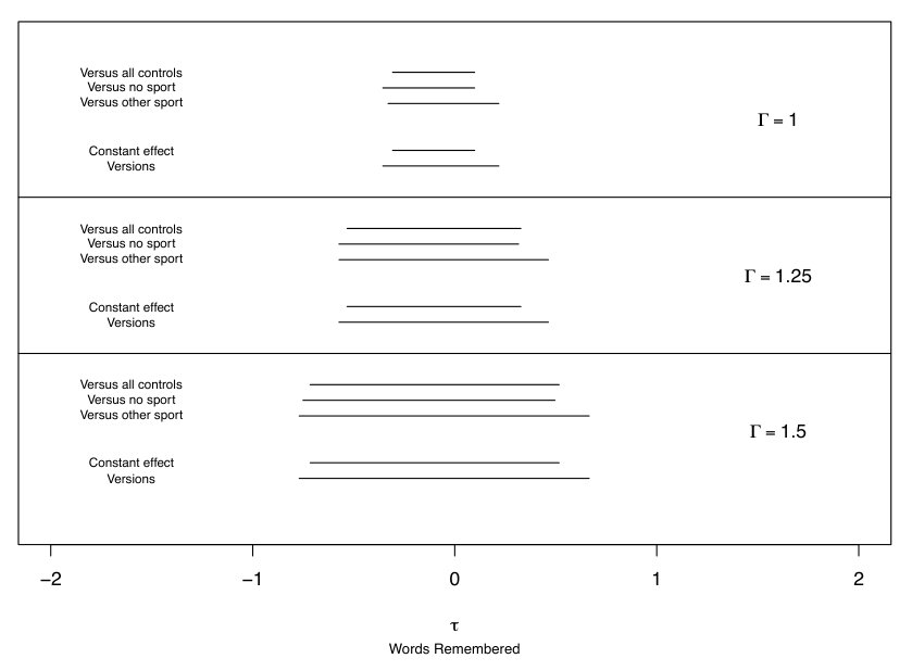 Figure 1
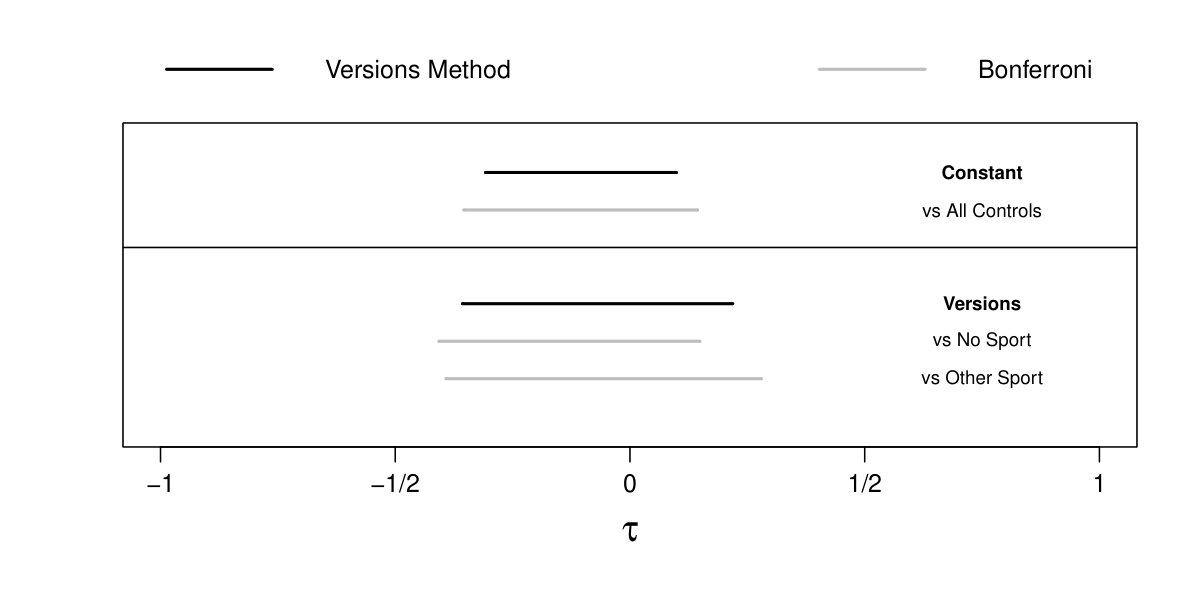 Figure 2
| Version | ||||
|---|---|---|---|---|
| 0.61 | 0.49 | 0.94 | 0.91 | |
| 0.58 | 0.47 | 0.93 | 0.88 | |
| 0.56 | 0.47 | 0.93 | 0.89 | |
| 0.51 | 0.43 | 0.89 | 0.85 | |
| 0.44 | 0.42 | 0.83 | 0.84 | |
| 0.44 | 0.44 | 0.83 | 0.86 | |
| 0.37 | 0.41 | 0.75 | 0.84 | |
| 0.27 | 0.55 | 0.58 | 0.95 | |
Peer Reviews
No public reviews on file for this paper yet. If you reviewed it on a platform where reviews are public (OpenReview, ICLR, NeurIPS, ICML), you can paste yours below so the community can read it here.
Videos
No videos yet. Explain this paper in a talk, walkthrough, or lecture? Add one.
Causal inference with two versions of treatment
Raiden B. Hasegawa, Sameer K. Deshpande, Dylan S. Small and Paul R. Rosenbaum111Raiden Hasegawa and Sameer K. Deshpande are PhD students and Dylan Small and Paul Rosenbaum are professors in the Department of Statistics, Wharton School, University of Pennsylvania, Philadelphia, PA 19104-6340 US. 31 May 2018. [email protected].
Abstract. Causal effects are commonly defined as comparisons of the potential outcomes under treatment and control, but this definition is threatened by the possibility that either the treatment or the control condition is not well-defined, existing instead in more than one version. This is often a real possibility in nonexperimental or observational studies of treatments, because these treatments occur in the natural or social world without the laboratory control needed to ensure identically the same treatment or control condition occurs in every instance. We consider the simplest case: either the treatment condition or the control condition exists in two versions that are easily recognized in the data but are of uncertain, perhaps doubtful, relevance, e.g., branded Advil vs. generic ibuprofen. Common practice does not address versions of treatment: typically the issue is either ignored or explicitly stated but assumed to be absent. Common practice is reluctant to address two versions of treatment because the obvious solution entails dividing the data into two parts with two analyses, thereby (i) reducing power to detect versions of treatment in each part, (ii) creating problems of multiple inference in coordinating the two analyses, (iii) failing to report a single primary analysis that uses everyone. We propose and illustrate a new method of analysis that begins with a single primary analysis of everyone that would be correct if the two versions do not differ, adds a second analysis that would be correct were there two different effects for the two versions, controls the family-wise error rate in all assertions made by the several analyses, and yet pays no price in power to detect a constant treatment effect in the primary analysis of everyone. Our method can be applied to analyses of constant additive treatment effects on continuous outcomes. Unlike conventional simultaneous inferences, the new method is coordinating several analyses that are valid under different assumptions, so that one analysis would never be performed if one knew for certain that the assumptions of the other analysis are true. It is a multiple assumptions problem, rather than a multiple hypotheses problem. We discuss the relative merits of the method with respect to more conventional approaches to analyzing multiple comparisons. The method is motivated and illustrated using a study of the possibility that repeated head trauma in high school football causes an increase in risk of early on-set cognitive decline.
Keywords: Causal effects, closed testing, full matching, intersection-union test, randomization inference, sensitivity analysis, versions of treatment.
1 What are versions of treatment?
Commonly, the effect on an individual caused by a treatment is defined as a comparison of the two potential outcomes that this individual would exhibit under treatment and under control; see Neyman (1923), Welch (1937) and Rubin (1974). Implicit in this definition is the notion that the treatment and control conditions are each well-defined. In particular, it is common to assume that there are “no versions of treatment or control”; see Rubin (1986).
By definition, versions of treatment are not intended additions to a study design, but rather potential flaws in the study design. Versions of treatment or control are often associated with finding treatments that occur naturally, rather than experimentally manipulating a tightly controlled, uniform treatment. Versions of one treatment should be distinguished from the intentional study of distinct, competing treatments. When an investigator discusses versions of one treatment, she is expressing a preference for the conception that there is a single treatment, but is acknowledging the possibility that her preferred conception is mistaken. Branded Advil and generic ibuprofen are versions of one treatment — possibly different, but very plausibly expected to be the same — whereas ibuprofen and aspirin are different competing treatments. The investigator and her audience prefer a primary analysis that does not distinguish versions of treatment, but both would be reassured by evidence that showed their preferred analysis does not embody a consequential error. Versions of control groups should also be distinguished from the deliberate use of two carefully selected control groups intended to reveal unmeasured biases if present; see, for instance, Rosenbaum (1987). In particular, Campbell (1969) suggested that two control groups should be deliberately selected to systematically vary a specific unmeasured covariate in an effort to demonstrate its irrelevance; however, versions of control are unintended flaws in study design, not purposeful quasi-experimental devices.
There are two versions of either the treatment condition or the control condition if we recognize in available data either two types of treated subjects or two types of controls, but we are uncertain about, or perhaps explicitly doubt, the relevance of this visible distinction. Versions refer to a visible but perhaps unimportant distinction, not to a distinction that is hidden or latent. There are important methodological issues in recognizing treatments that inexplicably affect some people but not others; however, this is practically and mathematically a different problem (Conover and Salsberg 1988; Rosenbaum 2007a).
In discussing randomized clinical trials, Peto et al. (1976, page 590-1) wrote: “A positive result is more likely, and a null result is more informative, if the main comparison is of only 2 treatments, these being as different as possible. … [I]t is a mark of good trial design that a null result, if it occurs, will be of interest.” This advice is equally relevant for observational studies, and it is part of the reason that we prefer a conception in which there is a single treated condition and a single control condition. Despite this, an investigator may seek some reassurance that the study’s conclusions cannot be undermined by the possibility of two versions of treatment.
In that spirit, our analysis focuses on the main treatment-control comparison, and subordinates the study of versions of treatment or versions of control. In particular, the main treatment-control comparison is unaffected by the exploration of versions of treatment — the usual confidence interval for a constant effect is reported — despite controlling the family-wise error rate in multiple comparisons that explore the possibility of versions of treatment with different effects. Two confidence intervals are reported, the usual interval for a constant effect and an interval designed to contain both effects if the two versions differ. If the effect is constant, then both intervals simultaneously cover that one effect with probability , but if there are two versions then the second interval covers both version effects with probability . The investigator always reports both intervals, valid under different assumptions. This is an unusual type of simultaneous inference: there is essentially one question, but there are two sets of assumptions underlying the answer, so one question is answered twice, as opposed to answering several different questions. There are multiple assumptions rather than multiple hypotheses. The two intervals together permit an investigator to report the conventional confidence interval for a constant effect, without lengthening it for multiple testing, yet the investigator also provides some information about whether the study’s conclusions depend on the absence of versions of treatment. The two intervals may possibly disagree, say about whether no effect is plausible, and if they do disagree then they demonstrate that the assumption about versions of treatment is playing an important role in the interpretation of the available data. Importantly, the method does not presume there is a single version of treatment by virtue of failing to reject the null hypothesis that the two versions are equal. That is, it entertains the possibility that there are versions of treatment even when the convetional interval assuming a constant treatment effect is not empty.
2 ** Possible versions of control in a study of football and dementia**
There is evidence that severe repeated head trauma accelerates the on-set of cognitive decline or dementia (Graves et al. 1990, Mortimer et al. 1991), with specific concern about the risks faced by professional football players and boxers (McKee et al. 2009, Lehman et al. 2012). It is unclear whether there is also increased risk from playing football on a team in high school, but there have been several recommendations against tackle football in high school (Bachynski 2016, Miles and Prasad 2016). Does high school football accelerate the on-set of cognitive decline?
A recent investigation used data from the Wisconsin Longitudinal Study, comparing cognition and mental health measured at age 65 and 72, recorded in 2005 and 2011, of men who played football on a high school team in the mid 1950’s to male controls of similar age who did not play football (Deshpande et al. 2017). Following the practice in clinical trials, and as is recommended for observational studies by Rubin (2007), the design and protocol for this study were published on-line after matching was completed but before outcomes were examined (Deshpande et al. 2016, arXiv preprint arXiv:1607.01756). The small number of people who engaged in sports other than football with high incidences of head trauma such as soccer, hockey, and wrestling were excluded from both the football and control groups. One outcome was the 0-10 score on a ten item delayed word recall (DWR) test at ages 65 and 72. The delayed word recall test was designed as an inexpensive measure of memory loss associated with dementia; see Knopman and Ryberg (1989). In this test, a person is asked to remember a list of words that is then read to the person. Attention then shifts to another activity, and after a delay, the person is asked to recall as many words from the list as possible. The DWR score is the number of words remembered. On average, in the Wisconsin Longitudinal Study, performance on the delayed word recall test declined by half a word from age 65 to age 72. It is useful to keep that half-word, 7-year decline in mind when thinking about the magnitude of the effect of playing football.
A comparison of football players to all controls is natural, and might be conducted without second thought. Among the controls, however, some played a non-collision sport like baseball or track while others played no sports at all. An investigator might reasonably seek reassurance that this natural comparison has not oversimplified these two version of “not playing football.” At the same time, the investigator does not want to sacrifice power to detect a constant treatment effect in the main comparison en route to obtaining this reassurance by subdividing the data into many slivers of reduced sample size and correcting for multiple comparisons. The method we propose achieves both of these objectives.
Our question concerns the effects of high school football. It is important to distinguish this question from questions about the effects of severe head trauma in general. It is at least conceivable that high school football is comparatively harmless, while severe head trauma is not, simply because severe head trauma is not common in high school football, and the benefits of exercise for all football players offset the harm of severe but rare trauma. Conversely, severe head trauma from automotive or other accidents may be difficult to prevent, but if high school football had grave consequences, then it could simply be banned, in the same way that most high schools do not have boxing teams. We ask about the effects of playing football in high school on subsequent cognitive function.
The Wisconsin Longitudinal Study describes a specific piece of the US over a specific period of time, and caution is advised about extrapolating its conclusions to other times and places. High School football may have changed since the 1950’s, and the demographic composition of Wisconsin in the 1950’s is not the demographic composition of the US. The Wisconsin Longitudinal Study is primarily a sequence of surveys, and it is impossible to use it to investigate questions not asked in those surveys. For instance, we cannot identify high school students who went on to play professional football, but we suspect they were few in number. Because many young people play high school football, the safety of high school football is an important question apart from the safety of professional football.
3 Full matching of football players and controls
We matched the 591 male football players to all 1,290 male controls who did not play football and did not play a contact sport. The match controlled for several factors that may affect later-life cognition, including the student’s IQ score in high school, their high school rank-in-class recorded as a percent, planned years of future education, as well as binary indicators of whether teachers rated him as an exceptional student, and whether his teachers and parents encouraged him to pursue a college education. We also accounted for aspects of family background like parental income and education.
The match was a “full match,” meaning that a matched set could contain one football player and one or more controls, or else one control and one or more football players. A full match is the form of an optimal stratification in the sense that people in the same stratum are as similar as possible subject to the requirement that every stratum contain at least one treated subject and one control; see Rosenbaum (1991). Although the proof of this claim requires some attention to detail, the key idea is simple: if a matched set contained two treated subjects and two controls, it could be subdivided into two matched sets that are at least as close on covariates and are typically closer. See Hansen and Klopfer (2006) for an algorithm for optimal full matching, Hansen (2007) for software, and Hansen (2004) and Stuart and Green (2008) for applications. The match was constructed using Hansen’s optmatch package in R with the ratio of controls to treated units constrained between 1:6 and 6:1 to avoid excessively large matched sets.
In a full match, there are matched sets, and individuals, , in set . If individual played on a football team in high school, write ; otherwise, write . The number of football players in set is , the total number of individuals is , and the total number of football players is . In a full match, for every .
To explore versions of treatment, we constructed three matched samples. Each sample used all football players. The first matched sample used all controls, that is, every male who played neither football nor another contact sport. The second matched sample used only controls who did not play any sport. The third matched sample used controls who played a non-collision sport, such as baseball. In each match, controls and football players belong to at most one matched set. Table 1 describes the structure of the three matched samples, giving the frequency of sets of size , as well as the number of sets, , the number of individuals, , and the number of football players, . Obviously, the samples overlap extensively, because they all use all football players and no controls were discarded in forming the optimal full matchings; however, the three matches differ in structure, partly because there were only controls who played a non-collision sport in the third match. In all three matches, adequate covariate balance was achieved with nearly all standardized differences in baseline covariates between football players and controls less than 0.2. Details of very similar matches can be found in Deshpande et al. (2017).
In studying the effects of a treatment — here, high school football — it is typically inappropriate to adjust for events subsequent to the start of treatment, as this may introduce bias even where none existed prior to adjustments, because part of the treatment effect may be removed (Rosenbaum 1984). However, there are certain adult health outcomes that may be different between football players and controls due to disparities in unmeasured baseline health characteristics rather than an effect of playing football. This may threaten the validity of our study if these baseline health characteristics also play a role in later-life cognitive health. Comparing these health outcomes may can be used, at least partially, to assess the comparability of the baseline health of the comparison groups. We checked on the health status of football players and matched controls at age 65 using the Mantel-Haenszel procedure, failing to find a difference significant at the 0.05 level for “ever had high blood pressure,” “ever had diabetes,” and “ever had heart problems”. Football players were more likely to report that they had “ever had a stroke,” with a -value of 0.03, and a 95% confidence interval for the odds ratio of . Extensive comparisons of this kind are reported in Deshpande et al. (2017).
4 Review of randomization inference without versions of treatment
If there were a single version of treatment or control, then individual would have two potential delayed word recall scores, if he played football and if he did not, where we observe only one of these, namely , and the effect caused by playing football, namely , is not observed for any individual; see Neyman (1923) and Rubin (1974). Fisher’s (1935) sharp null hypothesis of no effect says , , , which we henceforth abbreviate as , or as , . The treatment has an additive constant effect if there exists some constant such that , . The hypothesis specifies a particular numerical value for and asserts , , and it is manifested in the observable distribution of by a within-set shift in the distribution of by . If were true, then would satisfy Fisher’s hypothesis of no effect, , and it is commonplace to test by replacing by and testing .
Until §8, we restrict attention to random assignment of treatments within matched sets; however, §8 considers sensitivity of inferences to departures from this assumption. Of course, people do not decide to play football at random, so §8 is closer to reality than random assignment. Fisher (1935), Pitman and Welch (1937) used the randomization distribution of the mean difference to test Fisher’s , and we follow this approach with the short-tailed delayed word recall scores (DWR), only briefly comparing the mean to a robust -statistic. The mean is one -statistic, but not a robust one. Because the matched sets are of unequal sizes, , we compute the treated-minus-control mean difference in DWR scores within each set and combine them with efficient weights based on the matched set sizes; see Rosenbaum (2007b, §4.1) for discussion of these weights, which are implemented in the senfm function of the sensitivityfull package in R with option trim=Inf.
As is always true, a confidence interval for is formed by inverting a level- test, so is the shortest interval of values of not rejected by the test; see Lehmann and Romano (2005, §3) for general discussion. Typically, a two-sided confidence interval is the intersection of two one-sided confidence intervals; see Shaffer (1974).
Ignoring versions of treatment, using the first match in Table 1, and assuming that treatments are randomly assigned within matched sets, we obtain a randomization-based 95% confidence interval of for , that is, for a constant effect of playing football on the number of words remembered in the delayed word recall test. Because this confidence interval includes zero, the hypothesis of no effect is not rejected at the 0.05 level. Because this confidence interval excludes all with , constant effects of word remembered have been rejected as too large. It is important that “no effect” is plausible, but equally important that large effects, positive or negative, are implausible values for a constant effect, . Our goal is to avoid lengthening this interval for as we explore possible versions of the control, while controlling the family-wise error rate at , conventionally . This simultaneous inference is possible if the exploration of versions of treatment takes a specific form.
Incidentally, had we built the confidence interval for using the default -estimate in the senfm function, rather than the mean with option trim=Inf, then the 95% randomization interval for would have been . The default -estimate in senfm corresponds to Huber’s -function, i.e., for and for . Generally, use of robust procedures is advisable, but we do not do so in this example to simplify its presentation, as the robust procedures give similar answers in this short-tailed example.
5 Inference with versions of treatment
5.1 Structure of the problem
With two versions of control, say “playing no sport” and “playing a non-collision sport” like baseball, each person has two potential control responses, and , and hence two treatment effects, and . If , , then the two versions of control yield the same effects, , and so the versions need not be distinguished. This notation for potential outcome under versions of control follows Vanderweele and Hernan (2013) where potential outcomes are fixed by both treatment and version. If there are versions, the implied randomization distribution will have three arms when matched sets include both versions of control, which might complicate inference. However, we only use the matching with sets including both versions of control to conduct inference under the assumption that the versions are irrelevant, and thus the three arm randomization distribution collapses to the simpler two arm design.
Consider the two null hypotheses about additive effects for the two versions of control, , and , . Here, might be true when is false, or conversely. Define to be the hypothesis that both and are true, that is, , , so the two versions of control yield the same effect and need not be distinguished. By the definition of , if either or is false, then is false; that is, if there are two versions of treatment or control with different effects, then there is not a constant effect.
It is straightforward to test or using the methods in §4 simply by restricting attention to controls of one type or the other. These tests will be based on a smaller sample size than the test in §4 because not all of the controls are used. Moreover, if , and are each tested at level , then the chance of at least one false rejection would typically exceed unless something is done to control the family-wise error rate. Understandably, an investigator would like to avoid weakening the inference about by virtue of considering and , and the question is how to achieve the investigator’s goals.
Suppose there are two versions of a constant additive treatment effect, and for every . Let and . If , then and , so the versions do not matter. Our approach in §5.2 is to build two confidence intervals, one interval for and another interval designed to contain . If there is no need to consider versions of treatment or control because , implying that , then with probability at least , both intervals simultaneously cover the true . If , then is false for every , but with probability at least the second interval covers the interval . Moreover, the first interval for is the interval reported in §4 ignoring versions of treatment, so the investigator has ensured that under either the assumption of a constant treatment effect or the assumption of versions, the two intervals he reports control the family-wise error rate at , while paying no additional price in power to detect a constant effect for consideration of versions of treatment. The inference is simultaneous in that the two intervals provide the correct coverage for under the assumption of a constant effect and also the correct coverage for and under the presence of versions.
5.2 Inference when there may or may not be two versions of treatment
The theory in this section is derived for one-sided intervals but, as we will see shortly, is easily extended to the two-sided intervals described in the previous section. There is a valid, one-sided -value, say , testing against , so that if is true. In parallel, there is a valid one-sided -value , testing against , and a valid one-sided -value, , testing against . With a slight abuse of notation, write the probability that a random interval contains a fixed real number as . Under the assumption, perhaps incorrect, that the there is a single version of the treatment, , let be the usual one-sided confidence interval for formed by inverting the test of , so is the smallest set of the form containing . If there are no versions of treatment, so for some , then by the familiar duality of tests and confidence intervals; see Lehmann and Romano (2005, Chapter 3). The investigator would like to report this standard interval for a constant effect, without lengthening it for multiple testing, yet would like to also say something about the possibility that there are versions of treatment with . Of course, if there are versions of treatment with then is false for every and there is no true value of for to contain or omit.
The smallest set of the form containing will be denoted . Of course, .
The investigator does not know whether or not there are two versions of treatment, whether or not . The investigator would like to make two inferences appropriate for the two situations, or . The investigator would like to make an inference appropriate to this state of ignorance. The investigator says “I do not know whether there are two versions of treatment, whether or not ; however, (i) if there are not versions of treatment so that , then , and (ii) whether or not there are two versions of treatment, even if , then ; moreover, this method produces two true hypothetical statements with probability at least .” Statement (ii) cost nothing, in the sense that is the usual one-sided confidence interval for assuming there are not versions of treatment, yet both statements hold jointly without multiplicity correction. This is established in the following proposition.
Proposition 1
(i) If there is only one version of treatment, , then . (ii) In any event, whether there are two versions of treatment, , or only a single version, , we have .
Proof. By the definitions of and , we have . Then (i) follows because, if there are not versions of treatment, , then is a confidence interval for and . If there are not versions of treatment, , then , so , as required for (ii). So suppose there are two versions of treatment. If , then implies which occurs with probability at most . If , then implies which occurs with probability at most . So in all three cases, or or , we have , proving (ii).
By a parallel argument, we obtain analogous upper intervals, and , of the form for if or without restrictions for . Taking the intersections, and , of two one-sided intervals yields analogous two-sided intervals for if or without restrictions for the interval . In most cases, can be constructed by taking the union of and the two two-sided intervals constructed from the matched sets using each separate version of control. When this union is disjoint, is the shortest interval that contains all three intervals.
In case (ii), the proof above that is similar to, but not quite identical to, results in Lehmann (1952), Berger (1982) and Laska and Meisner (1989). These authors proposed tests that would invert to yield as a confidence interval the shortest interval containing , whereas is the shortest interval containing , thereby ensuring . Of course, , but unlike , our method ensures that and both simultaneously cover at rate when there is actually only a single version of treatment. Because is built using all of the data and under stronger assumptions, it is unlikely that will be much shorter than ; however, this logical possibility is the price for reporting the usual interval, , without multiplicity correction.
Why not report a single robust interval like instead of two intervals, and , that have slightly more nuanced coverage properties? A simple example may help illustrate the advantage of reporting and over . Suppose that and both contain zero but does not. If we choose to report then we have little additional information to determine why contains zero – is Fisher’s sharp null true or is the smaller of the the two versions of effect very close to zero? Or are there versions of the effect with different signs? However, if we report and we have evidence against Fisher’s sharp null, narrowing the plausible explanations for why zero is contained in , which we’ve noted will tend to be similar to .
5.3 Interval estimates in the football study
The upper third of Figure 1, marked , shows 95% intervals for the football study, assuming that treatments are randomly assigned within matched sets. First, there are the three conventional intervals for , , and , corresponding to the three comparisons in Table 1. Each of these intervals is a 95% confidence interval on its own, but each one runs a 5% chance of error, so the chance that at least one interval fails to cover its corresponding parameter is greater than 5%. Obviously, we could make the three intervals longer, say using the Bonferroni inequality, so that the simultaneous coverage is 95%, but many investigators would find this unattractive because it would reduce the power of the conventional, primary analysis focused on that uses all of the controls; that is, it would make the first interval longer.
In contrast, the intervals and in Figure 1 have simultaneous coverage of 95% in the sense of Proposition 1. Notably, is the interval for from §4, so consideration of has not reduced power to detect a constant effect. The versions is slightly longer than , but both intervals are compatible with no effect and both intervals are quite incompatible with an effect of half a word, . For comparison, recall from §2 that average performance on the delayed word recall test declined by half a word from age 65 to age 72. In Figure 1, the 95% interval for “all controls” equals , while is the union of the three intervals for “all controls”, “controls who played no sport”, and “controls who played another sport”.
6 Comparison to conventional approaches to multiple versions: F-tests and Bonferroni correction
The method described in §5.2 makes an important trade-off: it prioritizes the primary comparison against all controls under the assumption of a constant treatment effect, allowing us to report the corresponding confidence interval with no correction, in exchange for the ability to distinguish between versions if they do, in fact, exists. In other words, our method emphasizes detection of non-zero, constant treatment effects over detecting different versions of the effect. Conventional approaches to multiple comparisons, are often less focused and are designed to detect a broader range of departures from the null. For example, a simple Bonferroni correction places the primary comparison and the two versioned comparisons on equal footing. If the investigator does not suspect a priori that a particular alternative hypothesis is most likely, he may conduct an omnibus F-test, whose power is distributed over a broad range of alternative hypotheses.
The researcher’s scientifc aim should determine which method for multiple comparisons is most appropriate. With this guidance in mind, we compare our method to the omnibus F-test and Bonferroni corrected intervals.
The omnibus F-test
In exploratory analyses, the F-test can be a useful “prelude to subsequent examinations of unplanned contrasts” (Steiger, 2004). However, in many studies, the researcher will have a particular contrast in mind. Several authors have argued that the omnibus hypothesis in ANOVA studies be replaced with hypotheses that focus on a substantive research question, often involving just a single contrast (Rosenthal et al., 2000; Steiger, 2004). In the football study, we suspect a priori that versions are not terribly consequential and proceed first with our primary investigation of whether playing high school football accelerates the onset of cognitive decline. The hypotheses about versions are secondary to our main inquiry and are treated as such in our method.
The F-test does not lend itself to effect size estimates, but we can compare it to our method by evaluating it’s power to reject Fisher’s sharp null hypothesis and the probability that excludes under a variety of alternative hypotheses with vary degrees of “versioning.” If the primary goal of the study is less directed and detecting any departure from the null of no effect is of interest and the researcher suspects that versions may play an important role, the F-test may be more suitable. However, in a simulation study described in the Appendix, we find that when the versions differ by less than in magnitude and have the same sign our method has better power to reject Fisher’s sharp null than the F-test. Being an omnibus test, the F-test power is much less sensitive to the specific pattern of alternative hypothesis.
Bonferroni corrected intervals
In Figure 2, we compare the intervals returned by our version method to the three intervals returned by a Bonferroni correction (BC) to the comparison of the football players against all controls and each version of control. In the top panel, the BC interval using all controls is 22% longer than . In the bottom panel, is only 3% longer than the BC interval using only “no sport” controls and 15% shorter than the BC interval using “other sport” controls. In this particular case, where versions appear to be relatively innocuous, the cost of lengthening the primary interval is significant for what apears to be little if any gain from investigating each version separately. Bonferroni correction may be more appropriate when the investigator suspects the versions are important, and he may even replace the primary comparison with a comparison of the two versions of control themselves. However, if the versions are only modestly different, for which our method is designed, it is unlikely that Bonferroni would have sufficient power to detect such modest differences in the versions of control.
7 Versions, effect modification, and insufficient overlap
In the study of the effects of playing high school football on cognitive decline, the two versions of control and the football players have significant overlap in observed covariates. An anonymous reviewer suggested the following situation. Suppose that athletes who did not play football and non-athletes who did not play football differ noticeably on observed covariates such that a different set of football players were matched in the matchings using the different versions of control. If the treatment is heterogeneous, say it is modified by some observed covariate that differs between the two versions of control, does “this mean there are two versions of treatment or that there are two groups of individuals that are involved in the two comparisons.” In this setting, the potential for treatment heterogeneity is aliased with the potential for versions of the treatment effect. But does this matter? The logic of §5.2 is agnostic to why there may be different treatment effects between versions. Thus, can be interpreted as assessing how robust our primary analysis is to the existence of versions of treatment or to the existence of effect heterogeneity between the two groups defined by “versions” of control.
8 Sensitivity to departures from random assignment
So far, we have drawn inferences under the assumption that treatments are randomly assigned within matched sets. In an observational study, this assumption lacks support and is typically doubtful if not implausible. We examine sensitivity to bias from nonrandom assignment by assuming that two individuals with the same observed covariates may differ in their odds of treatment by at most a factor of due to differences in unobserved covariates; see Rosenbaum (2007b; 2017, §9). This yields hypothesis tests that falsely reject a true null hypothesis with probability at most when the bias in treatment assignment is at most . Then is varied to display the magnitude of bias that would need to be present to alter the conclusions of a study. How much bias, measured by , would need to be present to lead us to fail to reject the null hypothesis of no effect of football when, in fact, football causes substantial harm? In the current example where there is no evidence of a harmful effect of football, we may ask a parallel question that is related to equivalence testing: how much bias would need to be present to mask a substantial true effect of football on memory? For example, an increase or decrease of a DWR score by at least one word.
Aids to interpreting values of are discussed by Rosenbaum and Silber (2009) and Hsu and Small (2013). In particular, in a matched pair with , the value corresponds with an unobserved covariate that doubles the odds of playing football and doubles the odds of a worse memory score, while corresponds with an unobserved covariate that doubles the odds of playing football and quadruples the odds of a worse memory score; see Rosenbaum and Silber (2009) and Rosenbaum (2017, §9). Proposition 1 applies to the intervals obtained from upper bounds on -values from sensitivity analyses, providing the bias in treatment assignment is at most .
Figure 1 shows the expansion of and as increases from for randomization inferences to and . For , the intervals are and . For , the intervals are and . A bias of together with two versions of not playing football would be insufficient to mask an effect of one word on the memory test, . At , not shown in Figure 1, effects of word start to be included in the confidence intervals, with and . A bias of corresponds with an unobserved covariate that triples the odds of playing football and increases the odds of worse memory performance by five-fold.
In brief, there is no sign of an effect of high school football on memory scores. Could the absence of any sign of an effect reflect a substantial effect and bias in who plays football? To mask a true effect of word, an unobserved bias would have to be moderately large, . Even allowing for both moderate confounding due to unmeasured covariates and versions of treatment, large effects of high school football on memory scores are not consistent with the data.
9 **Discussion: Simultaneous inference about one question under different
assumptions**
Investigators sometimes candidly report two or more statistical analyses valid under different assumptions. In the process, they often lose the several advantages of a single, simple, primary analysis, that is, a single analysis with high power against a non-zero constant effect because it uses everyone and avoids needed corrections for multiple testing when several statistical tests are performed. With less candor, investigators sometimes perform several analyses and report some but not all analyses, a perhaps common practice that no one would publicly advocate.
Versions of treatment arise in observational studies when treatment or control conditions found in available data may not be uniform, as they would be in a tightly controlled experiment. The investigator would like follow the practice of clinical trials and report a single, primary analysis using everyone without multiplicity correction. Nonetheless, the investigator would like to speak to the possibility that there are versions of treatment or control conditions. The proposed method always reports two interval estimates. The first, shorter interval, , is precisely the interval that would be reported in a single primary analysis without versions of treatment. The second longer interval, , attempts to cover both treatment effects if there are two versions of treatment or two versions of control. If there is, in fact, only a single treatment effect, the same for both versions, then the probability that both and simultaneously cover that one effect is the stated rate of . If there are, in fact, two treatment effects that differ with the two versions, then the second interval, , covers both effects with the stated rate of . In that sense, the added information provided by reporting two intervals, \mathcal{I}_{c}\and , is free: the interval is clarified but not lengthened by examining . Although is always somewhat longer than , in the football example it is only slightly longer, thereby suggesting that the primary analysis is not greatly distorted by the two versions of the control condition.
References
Bachynski, K. E. (2016), “Tolerable risks? physicians and tackle football,” New England Journal of Medicine, 374, 405-407.
Berger, R. L. (1982), “Multiparameter hypothesis testing and acceptance sampling,” Technometrics, 24, 295-300.
Campbell, D. T. (1969), “Prospective: Artifact and Control,” in R. Rosenthal and R. L. Rosnow, eds., Artifact in Behavioral Research, New York: Academic Press, 351-382.
Conover, W. J. and Salsburg, D. S. (1988), “Locally most powerful tests for detecting treatment effects when only a subset of patients can be expected to respond to treatment,” Biometrics, 44, 189-196.
Deshpande, S.K., Hasegawa, R.B., Rabinowitz, A.R., Whyte, J., Roan, C.L., Tabatabaei, A., Baiocchi, M., Karlawish, J.H., Master, C.L., and Small, D.S. (2017), “High school football and later life cognition and mental health: An observational study,” JAMA Neurology, 74, 909-918. Protocol for study 2016: arXiv preprint arXiv:1607.01756.
Fisher, R. A. (1935), The Design of Experiments, Edinburgh: Oliver & Boyd.
Graves, A. B., White, E., Koepsell, T., Reier, B. V., Van Belle, G., Larson, E. B., and Raskind, M. (1990), “The association between head trauma and Alzheimer’s disease,” American Journal of Epidemiology, 131, 491-501.
Hansen, B. B. (2004), “Full matching in an observational study of coaching for the SAT,” Journal of the American Statistical Association, 99, 609-618.
Hansen, B. B. and Klopfer, S. O. (2006), “Optimal full matching and related designs via network flows,” Journal of Computational and Graphical Statistics, 15, 609-627. (R package optmatch)
Hansen, B. B. (2007), “Flexible, optimal matching for observational studies,” R News, 7, 18-24. (R package optmatch)
Hsu, J. Y. and Small, D. S. (2013), “Calibrating sensitivity analyses to observed covariates in observational studies,” Biometrics, 69, 803-811.
Knopman, D. S. and Ryberg, S. (1989), “A verbal memory test with high predictive accuracy for dementia of the Alzheimer type,” Archives of Neurology, 46, 141-145.
Laska, E. M. and Meisner, M. J. (1989), “Testing whether an identified treatment is best,” Biometrics, 45, 1139-1151.
Lehman, E. J., Hein, M. J., Baron, S. L., and Gersic, C. M. (2012), “Neurodegenerative causes of death among retired national football league players,” Neurology, 79, 1970-1974.
Lehmann, E. L. (1952), “Testing multiparameter hypotheses,” Annals of Mathematical Statistics, 23, 541-552.
Lehmann, E. L. and Romano, J. (2005), Testing Statistical Hypotheses (3rd edition), New York: Springer.
Miles, S. H. and Prasad, S. (2016), “Medical ethics and school football,” American Journal of Bioethics, 16, 6-10.
McKee, A. C., Cantu, R. C., Nowinski, C. J., Hedley-Whyte, T., Gavett, B. E., Budson, A. E., Santini, V. E., Lee, H.-S., Kublius, C. A., and Stern, R. A. (2009), “Chronic traumatic encephalopathy in athletes: progressive tauopathy after repetitive head injury,” Journal of Neuropathology and Experimental Neurology, 68, 709-735.
Mortimer, J. A., van Duijn, C. M., Chandra, V., Fratiglioni, L., Graves, A. B., Heyman, A., Jorm, A. F., Kokmen, E., Kondo, K., Rocca, W. A., Shalat, S. L., Soininen, H., and for the Eurodem Risk Factors Research Group (1991), “Head trauma as a risk factor for alzheimer’s disease: a collaborative re-analysis of case-control studies,” International Journal of Epidemiology, 20, S28-S35.
Neyman, J. (1923, 1990), “On the application of probability theory to agricultural experiments,” Statistical Science, 5, 463-480.
Peto, R., Pike, M., Armitage, P., Breslow, N. E., Cox, D. R., Howard, S.V., Mantel, N., McPherson, K., Peto, J. and Smith, P.G. (1976), “Design and analysis of randomized clinical trials requiring prolonged observation of each patient. I. Introduction and design,” British Journal of Cancer, 34, 585-612.
Pitman, E. J. (1937), “Statistical tests applicable to samples from any population,” Journal of the Royal Statistical Society, 4, 119-130.
Rosenbaum, P. R. (1984), “The consquences of adjustment for a concomitant variable that has been affected by the treatment,” Journal of the Royal Statistical Society, A, 147, 656-666.
Rosenbaum, P. R. (1987), “The role of a second control group in an observational study,” Statistical Science, 2, 292-306.
Rosenbaum, P. R. (1991), “A characterization of optimal designs for observational studies,” Journal of the Royal Statistical Society B, 53, 597-610.
Rosenbaum, P. R. (2007a), “Confidence intervals for uncommon but dramatic responses to treatment,” Biometrics, 63, 1164-1171.
Rosenbaum, P. R. (2007b), “Sensitivity analysis for m-estimates, tests and confidence intervals in matched observational studies,” Biometrics, 63, 456-464. (R package sensitivitymult; demonstration at https://rosenbap.shinyapps.io/learnsenShiny/)
Rosenbaum, P. R. and Silber, J. H. (2009), “Amplification of sensitivity analysis in observational studies,” Journal American Statistical Association, 104, 1398-1405. (amplify function in the R package sensitivitymult)
Rosenbaum, P. R. (2017), Observation and Experiment: An Introduction to Causal Inference, Cambridge, MA: Harvard University Press.
Rosenthal, R., Rosnow, R. L., and Rubin, D. B. (2000), Contrasts and effect sizes in behavioral research: A correlational approach, New York, NY: Cambridge University Press.
Rubin, D. B. (1974), “Estimating causal effects of treatments in randomized and nonrandomized studies,” Journal of Educational Psychology, 66, 688-701.
Rubin, D. (1986), “Comment: Which ifs have causal answers,” Journal of the American Statistical Association, 81, 961-962.
Rubin, D. B. (2007), “The design versus the analysis of observational studies for causal effects: parallels with the design of randomized trials,” Statistics in Medicine, 26, 20-36.
Shaffer, J. P. (1974), “Bidirectional unbiased procedures,” Journal of the American Statistical Association, 69, 437-439.
Steiger, J. H. (2004), “Beyond the F Test: Effect Size Confidence Intervals and Tests of CLose Fit in the Analysis of Variance and Contras Analysis, ” Psychological Methods, 9(2), 164-182.
Stuart, E. A. and Green, K. M. (2008), “Using full matching to estimate causal estimates in nonexperimental studies: examining the relationship between adolescent marijuana use and adult outcomes,” Developmental Psychology, 44, 395-406.
VanderWeele, T. J. and Hernan, M. A. (2013), “Causal Inference Under Multiple Versions of Treatment, ” Journal of Causal Inference, 1(1), 1-20.
Welch, B. L. (1937), “On the z-test in randomized blocks and Latin squares,” Biometrika, 29, 21-52.
Appendix: Simulation comparing the power of the omnibus F-test to
In this appendix, we compare the power of the omnibus F-test to the power of our version method to detect departures from Fisher’s sharp null hypothesis under varying degrees of “versioning.” The results can be found in Table 2. When the degree of versioning is modest, the version method is more powerful than the F-test.
Simulation settings
Let there be matched sets, with treated and controls in each set. The design is balanced over versions, i.e., there are two controls of each version in each matched set. In each set we generate outcomes as follows: if the -th subject in set receives treatment, if the -th subject receives control version , and if the -th subject receives control version. We let the individual and matched-set level terms, and , be distributed as independent standard normals. Finally, let and . If there are no versions, then . When conducting the F-test of the null of no treatment effect, we model as a linear effect.