Asymptotic Formulae for Mixed Congruence Stacks
Richard Frnka

TL;DR
This paper extends the circle method to derive asymptotic formulas for mixed congruence unimodal sequences, revealing their growth behavior and distribution properties.
Contribution
It introduces new asymptotic expansions for mixed congruence unimodal sequences using Wright's circle method and modular transformations.
Findings
Asymptotic formulas for mixed congruence unimodal sequences derived
Techniques include Wright's circle method and modular transformations
Provides detailed asymptotic behavior of these sequences
Abstract
Much like the important work of Hardy and Ramanujan proving the asymptotic formula for the partition function, Auluck and Wright gave similar formulas for unimodal sequences. Following the circle method of Wright, we provide the asymptotic expansion for unimodal sequences on a two-parameter family of mixed congruence relations, with parts on one side up to the peak satisfying r (mod m) and parts on the other side -r (mod m). Techniques used in the proofs include Wright's circle method, modular transformations, and bounding of complex integrals.
Click any figure to enlarge with its caption.
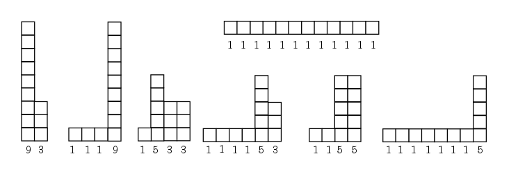 Figure 1
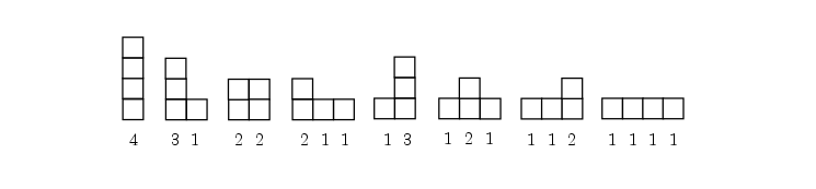 Figure 2
Peer Reviews
No public reviews on file for this paper yet. If you reviewed it on a platform where reviews are public (OpenReview, ICLR, NeurIPS, ICML), you can paste yours below so the community can read it here.
Videos
No videos yet. Explain this paper in a talk, walkthrough, or lecture? Add one.
Asymptotic Formulae for Mixed Congruence Stacks
Richard Frnka
Department of Mathematics
Louisiana State University
Baton Rouge, LA 70802
U.S.A.
Abstract.
Much like the important work of Hardy and Ramanujan [12] proving the asymptotic formula for the partition function, Auluck [6] and Wright [21] gave similar formulas for unimodal sequences. Following the Circle Method of Wright, we provide the asymptotic expansion for unimodal sequences on a two-parameter family of mixed congruence relations, with parts on one side up to the peak satisfying and parts on the other side . Techniques used in the proofs include Wright’s Circle Method, modular transformations, and bounding of complex integrals.
Key words and phrases:
false theta functions; stacks; unimodal sequences; Wright circle method
2010 Mathematics Subject Classification:
05A15, 05A16, 05A17, 11P81, 11P82.
1. Introduction and Statement of Main Results
Hardy and Ramanujan [12] provided an asymptotic expansion of the partition function for large , showing the exponential growth of :
[TABLE]
When adding restrictions to the parts so that each part is and letting count these partitions, an asymptotic formula given by Meinardus [16] is
[TABLE]
With the parts allowed to be and letting be the number of partitions, Livingood [15] showed
[TABLE]
The generating functions for these partition relations involve infinite -series and manipulations of the Circle Method are used in the proofs. Beckwith and Mertens [7] have also proven other variations involving the multiplicity of parts appearing in residue classes.
We extend these ideas to unimodal sequences, where the restriction on non-increasing ordering of parts for partitions is slightly relaxed.
Definition**.**
A unimodal sequence or stack of size is a sequence of non-zero parts , , and such that
[TABLE]
and
[TABLE]
We let be the number of stacks of size and show the unimodal sequences of size in Figure 1.
Questions about the asymptotics for the stack function were first introduced by the physicist Temperley [19] in 1951, who was studying particle configurations on specific lattices. The entropy of the system depends on the exponential bound of , which had not been previously discovered. This was provided by Auluck in 1951 [6], when he showed
[TABLE]
This was proved using a different method by Wright in 1971 [21] and he also gave a way to calculate lower order terms, providing the asymptotic expansion in powers of .
In [4], Andrews examined some interesting cases of concave and convex unimodal sequences. He defined a “mixed parity” case where on one side of the stack the parts are odd, with even parts on the other side. A detailed study of the combinatorial and asymptotic behavior of unimodal sequences with parity conditions will be the subject of a subsequent paper.
Definition**.**
A mixed congruence stack is a unimodal sequence satisfying (1.1) and (1.2), as well as congruence relations on the parts where for , gcd, and ,
[TABLE]
Letting be the number of mixed congruence stacks of size , the generating function is
[TABLE]
where we are following the standard -series notation
[TABLE]
The index in the generating function refers to the height of the peak at . Then we have parts up to on the left and parts up to on the right of the stack. Shown in Figure 2, we see the mixed stacks for the relation of size .
Theorem 1.1**.**
For ,
[TABLE]
Remark*.*
Note that Theorem 1.1 applies for , but when , there is a missing part of the congruence on the right side of the stack. In this case, the term is less than the peak at but is absent, creating a gap. The generating function that fills the gap when can be analyzed separately
[TABLE]
Remark*.*
In the case , a pole is introduced so it is excluded by adding the requirement . Note that the exponential term of Theorem 1.1 for matches (1.3) although the constant terms are different.
Remark*.*
The proof of Theorem 1.1 uses the Circle Method developed by Wright in [21] and [22]. It is important to note that Ngo and Rhoades have recently proven a general version of Wright’s approach. Propositions 1.8 - 1.10 of [17] are widely applicable to functions of the shape , where has an exponential singularity near , and has an asymptotic expansion. Read in the context of Proposition 1.8 from [17], the bulk of the work in Section 3 of this paper is devoted to verifying HYPO 4 from Ngo-Rhoades, as the infinite product that occurs here must be analyzed separately near roots of unity.
Example*.*
For the case and , we have
[TABLE]
Letting the first term in our asymptotic formula be
[TABLE]
we can see the accuracy of the theorem statement in Table 1 based on relative error.
The generating function is rewritten in terms of an infinite -series product and a false theta function. A modular transformation is established for the -series and an asymptotic expansion is given for the false theta function. Details are in Section 2.
Once we have the transformation formula, Section 3 proceeds to evaluate the coefficients by Cauchy’s formula. Wright’s Circle Method is used to give the asymptotic formula for the integral and thus mixed congruence stacks.
Acknowledgements
This work is a result of the author’s Ph.D. Thesis at Louisiana State University. Special thanks to Karl Mahlburg for advising on the project, providing knowledge on the subject, and pointing to excellent references. The author also thanks the two anonymous referees for their many helpful comments and thoroughness in reviewing this paper.
2. Hypergeometric -series and Theta Functions
As in the work of Wright [21] on ordinary unimodal sequences, we must transform the generating function.
Proposition 2.1**.**
[TABLE]
Proof.
One of the equations from Ramanunjan’s Lost Notebook representing the unimodal-rank generating function is explored in depth in [2] as Equation (1.1):
[TABLE]
This equation is a special case of Heine’s transformation formula for hypergeometric series. Sending and , multiplying by and reorganizing in (2.2) completes the proof. ∎
We wish to analyze individually the different pieces of the right hand side of (2.1), so we let
[TABLE]
where
[TABLE]
The term only offers a contribution of for high order terms, so letting be the main term, we have that for .
With the generating series in this particular form, we can turn our attention to each individual piece. The sum is a false theta function whose coefficients can be bounded, and the infinite -series satisfies a modular transformation formula. The transformation formula will provide a first term in the asymptotic expansion of that will be vital for the circle and function over which we will be integrating.
Proposition 2.2**.**
For and , as ,
[TABLE]
Proof.
The function can be expressed in terms of Jacobi’s theta function (see [10] for a good reference), which is
[TABLE]
and has an equivalent product form by the Triple Product Identity,
[TABLE]
The theta function satisfies the following transformation formulas:
[TABLE]
The Dedekind eta function satisfies the inversion formula
[TABLE]
We can express our function in terms of the theta functions under a nice transformation.
We have for and , that
[TABLE]
Letting and in (2.7),
[TABLE]
where by plugging in for and for in (2.5), we have
[TABLE]
Using the inversion formula (2.8), we also have that
[TABLE]
so
[TABLE]
Finally, plugging (2.11) and (2.13) into (2.9), we have
[TABLE]
∎
False theta functions do not satisfy the same functional equations as the typical theta function, although they have the same shape. Euler-Maclaurin summation can be used to expand out in desired powers of , but we use a result found in [14], where the authors explored the function
[TABLE]
and showed the following:
Lemma 2.3** (Kim, Kim, Seo (2015)).**
For , as with ,
[TABLE]
where .
If we let in (2.15), then
[TABLE]
Now letting and , we can find constants for the false theta function in powers of up to a desired degree , as in Lemma 1 of [21].
Lemma 2.4**.**
For where is some arbitrary constant, taking gives
[TABLE]
where
[TABLE]
3. Wright’s Circle Method and Proof of Theorem 1.1
The proof follows the notation and method of Wright in [21]. We let replace and send . Then the modular transformation in Proposition 2.2 becomes
[TABLE]
Defining
[TABLE]
the following term is critical for the Circle Method
[TABLE]
Using the Arithmetic-Geometric Mean Inequality on the exponent above gives
[TABLE]
where equality occurs when with
[TABLE]
The circle of radius centered at [math] will be the contour of integration. The major arc is defined to be where arg for small fixed . The minor arc is the rest of the circle , away from the pole at .
We can now use the Circle Method over , establishing the integral
[TABLE]
which will be approximated by with the constants from Lemma 2.18 and
[TABLE]
The main term of each will be shown to be where
[TABLE]
Proposition 3.1**.**
For , , and as ,
[TABLE]
Proof.
Breaking up the difference of the integrals into 3 pieces, we have
[TABLE]
Note that
[TABLE]
and letting on the circle , the real part of is , so
[TABLE]
Over , we see that . Along with Lemma 2.18,
[TABLE]
[TABLE]
The modular inversion formula in (3.1) shows that
[TABLE]
Asymptotically, (3.6) really tells us that on
[TABLE]
Hence we can bound by using (3.5), (3.8), and (3.9):
[TABLE]
As we move away from the pole at along the minor arc, there are still some problematic spots, specifically at th roots of unity. Firstly, suppose on is not close to a root of unity. Explicitly, we have that and want to insure that is sufficiently far away from a root of unity, thus we require for that
[TABLE]
Now we can use the logarithm for an asymptotic expansion:
[TABLE]
The Taylor Series Expansion for is
[TABLE]
so the above becomes
[TABLE]
The sum on the right is a geometric series, so
[TABLE]
Taking the absolute value, we can bound the log term:
[TABLE]
where we have pulled out the term and added and subtracted in a term. As , we rearrange the sum and see
[TABLE]
Now , so by our modular inversion formula (3.1),
[TABLE]
On , we know , so
[TABLE]
and by using the Taylor expansion of , one can approximate
[TABLE]
Plugging (3.14), (3.15), and (3.16) into (3.13), we have that
[TABLE]
Finally, we can bound :
[TABLE]
The goal was to beat the bound , hence we have motivated the choice for the constant and have successfully bounded under the assumption that was away from a root of unity.
Suppose now that is close to an th root of unity and (otherwise we can reduce the case down). Following the techniques used by Bringmann and Mahlburg in [9], we want to shift away from the root of unity by a small amount that still allows us to use the periodicity of the theta functions.
The th roots of unity for are near for . Thus we consider for some so that . With this shift in mind, we can rewrite
[TABLE]
where and . Then we can write in terms of :
[TABLE]
where is the fractional part (this will be nonzero since gcd). Then we can express this in terms of theta and eta functions:
[TABLE]
Now using the transformations of the theta (2.7) and eta (2.8) functions in (3.22), we have
[TABLE]
For the eta function, the approximation is
[TABLE]
and for the theta function,
[TABLE]
Putting (3.24) and (3.25) into (3.23), the main exponential term becomes
[TABLE]
Bounding this term and noticing that for ,
[TABLE]
hence we still receive our exponential savings over . ∎
Lastly, we need to bound the approximating integral , and calculate out the final asymptotic result.
Proposition 3.2**.**
For and ,
[TABLE]
Proof.
Let be the rectangle whose endpoints are (traversed counter-clockwise). Then we define
[TABLE]
since the integral over is exactly the image of in the plane, hence
[TABLE]
Sending , the integral representation for the modified Bessel function appears (obtained by using the transformation on the loop integral for found on page 355 of [20]):
[TABLE]
In the plane on the contour , the endpoints of the rectangle are now given by . Consider the integral on :
[TABLE]
If we let , then , so . This function is increasing on the interval, so it achieves a maximum value when . Thus
[TABLE]
Similarly on and , the integrals are . ∎
Remark*.*
As for all , the error term is indeed smaller than the main term.
We have . If we use Hankel’s approximation for the Bessel function (for a good reference, see [1]), we can write
[TABLE]
From Proposition 3.1,
[TABLE]
and plugging (3.26) into (3.27) and pulling out the first term,
[TABLE]
for constants . Finally, , and when , the coefficients , hence
[TABLE]
As , we have effectively determined the asymptotic expansion for mixed congruence stacks. The terms are insignificant compared to , so we can drop them, completing the proof of Theorem 1.1.
The reference list from the paper itself. Each links out to its DOI / PubMed record.
- 1[1] M. Abramowitz and I.A. Stegun,“Modified Spherical Bessel Functions.” §10.2 in Handbook of Mathematical Functions , 9 9 9 th printing. New York: Dover, pp. 443-445, 1972.
- 2[2] G. Andrews, “An Introduction to Ramanujan’s ‘Lost’ Notebook”, Ramanujan: Essays and Surveys (AMS) 22 , Providence, RI (2001) 165-184
- 3[3] G. Andrews, The Theory of Partitions , Cambridge University Press, Cambridge, 1998.
- 4[4] G. Andrews, “Concave and Convex Compositions,” Ramanujan J. 31 (2013), no. 1-2, 67-82.
- 5[5] G. Andrews, “Ramanujan’s ‘lost’ notebook I: Partial θ 𝜃 \theta -functions.” Adv. in Math. 41 (1981), no. 2, 137-172.
- 6[6] F. Auluck, “On Some New Types of Partitions Associated with Generalized Ferrers Graphs,” Math. Proc. Cambridge Philos. Soc. , 47 (1951) 679-686.
- 7[7] O. Beckwith and M. H. Mertens , “The Number of Parts in Certain Residue Classes of Integer Partitions”, Res. Number Theory 1 no. 11 (2015) 1-15.
- 8[8] K. Bringmann and K. Mahlburg, “Asymptotic Formulas for Stacks and Unimodal Sequences,” J. Combin. Theory Ser. A 126 (2014) 194-215.