Model Order Reduction for Rotating Electrical Machines
Zeger Bontinck, Oliver Lass, Sebastian Sch\"ops, Oliver Rain

TL;DR
This paper develops an adaptive model order reduction method using proper orthogonal decomposition for simulating non-symmetric rotating electrical machines efficiently, with error certification and demonstrated effectiveness.
Contribution
It introduces an adaptive reduction technique specifically tailored for non-symmetric machines, addressing challenges not covered by existing symmetric models.
Findings
Effective reduction of simulation costs for non-symmetric machines
Error estimator certifies solution accuracy
Numerical examples validate the method's efficiency
Abstract
The simulation of electric rotating machines is both computationally expensive and memory intensive. To overcome these costs, model order reduction techniques can be applied. The focus of this contribution is especially on machines that contain non-symmetric components. These are usually introduced during the mass production process and are modeled by small perturbations in the geometry (e.g., eccentricity) or the material parameters. While model order reduction for symmetric machines is clear and does not need special treatment, the non-symmetric setting adds additional challenges. An adaptive strategy based on proper orthogonal decomposition is developed to overcome these difficulties. Equipped with an a posteriori error estimator the obtained solution is certified. Numerical examples are presented to demonstrate the effectiveness of the proposed method.
Click any figure to enlarge with its caption.
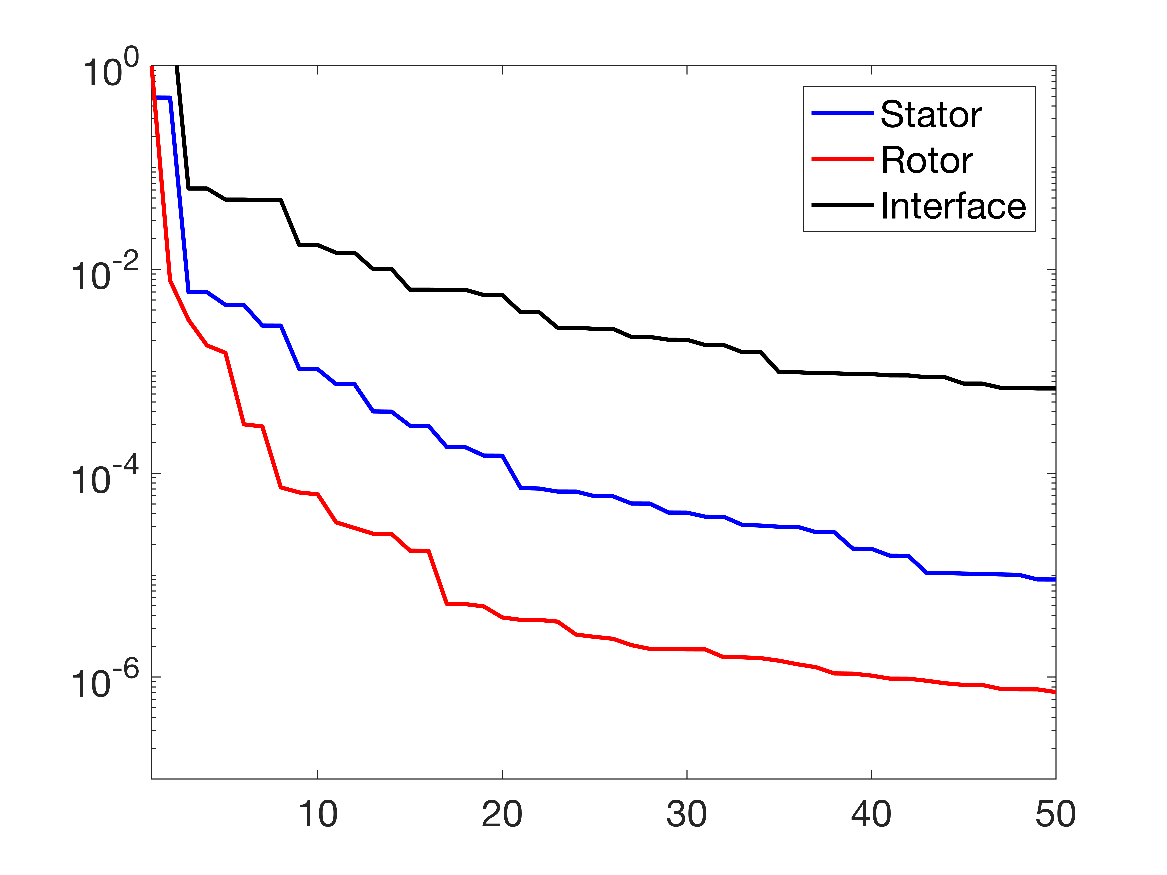 Figure 1
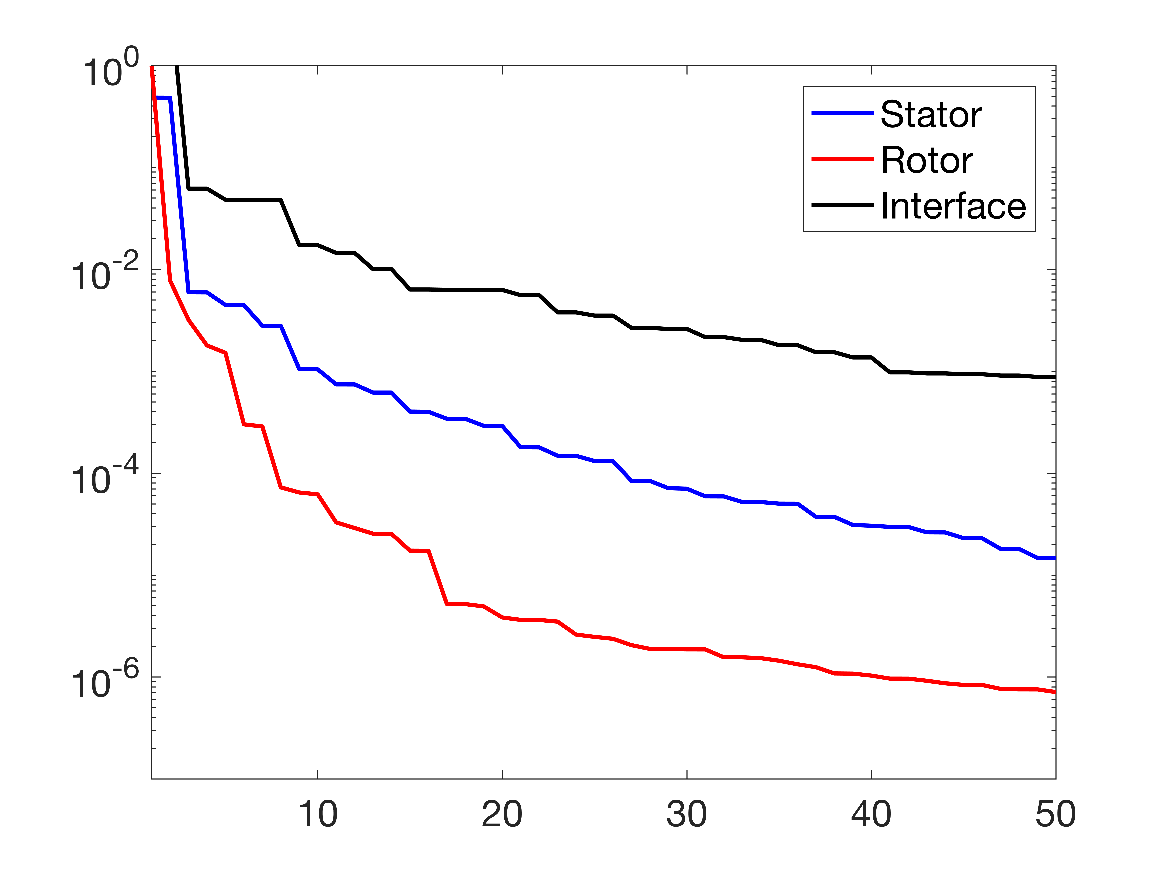 Figure 2
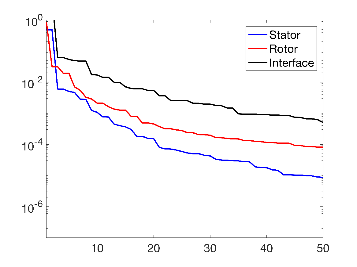 Figure 3
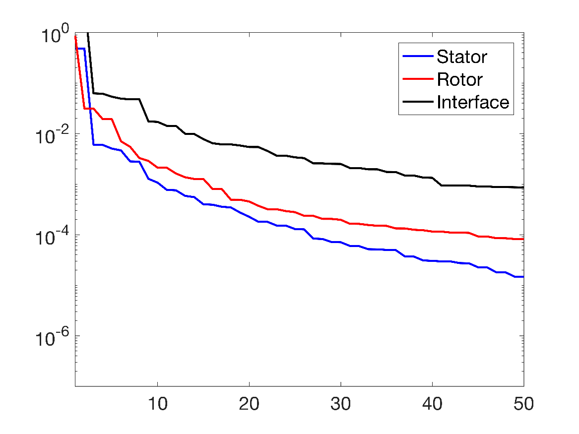 Figure 4
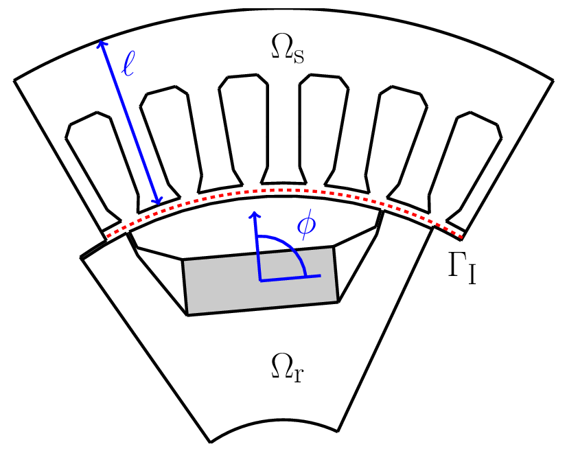 Figure 5
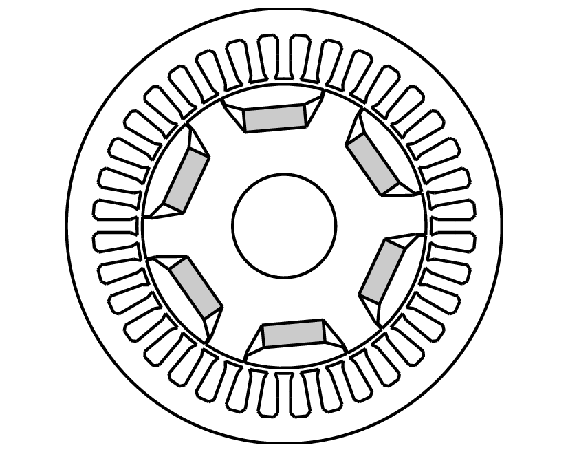 Figure 6
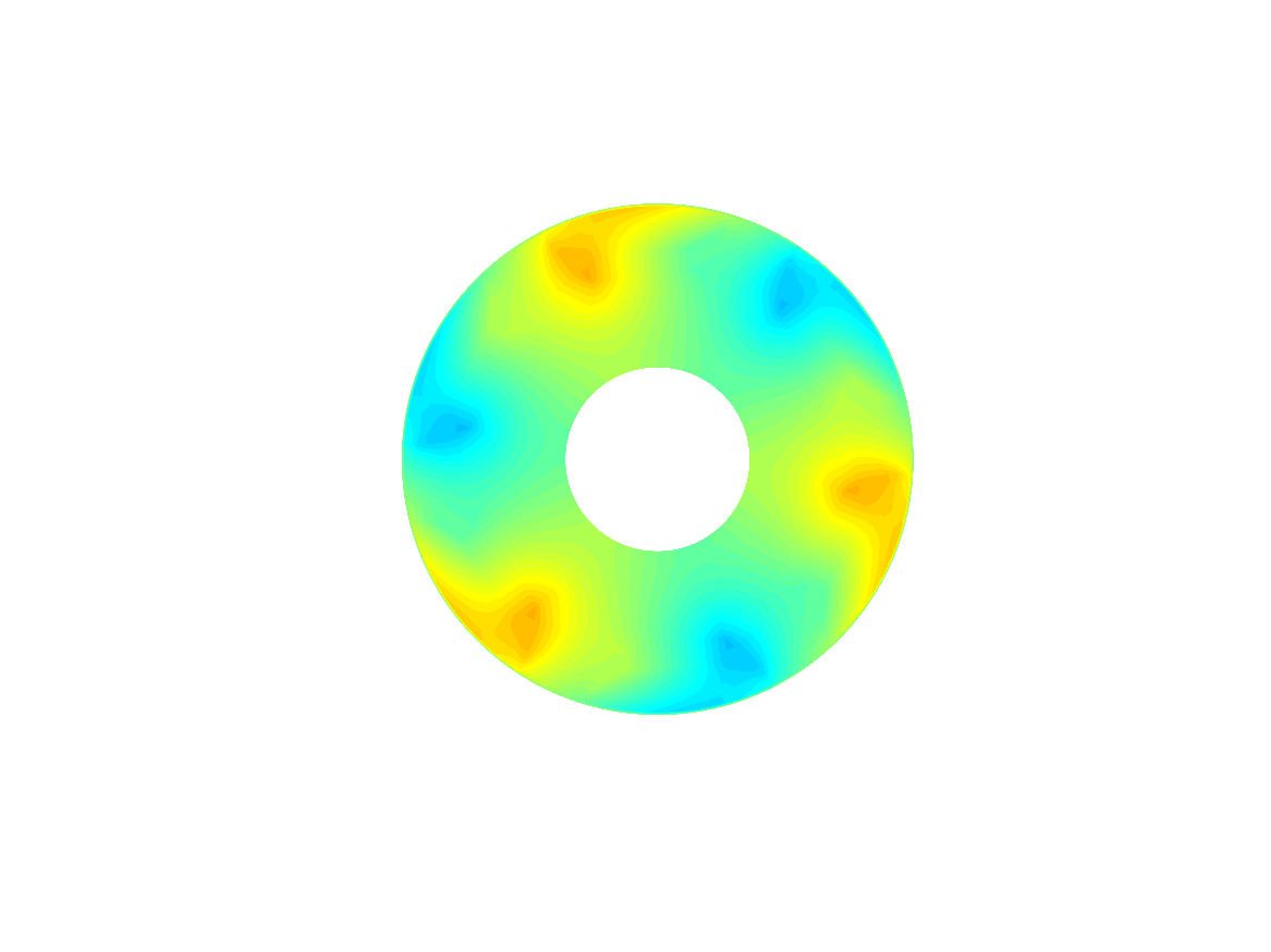 Figure 7
 Figure 8
 Figure 9
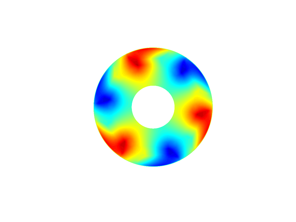 Figure 10
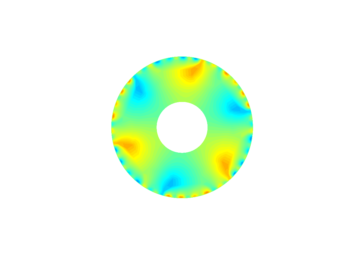 Figure 11
 Figure 12
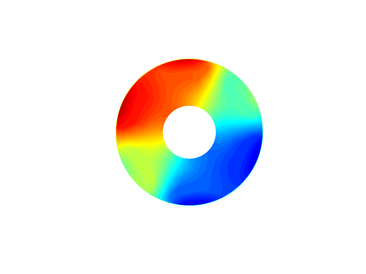 Figure 13
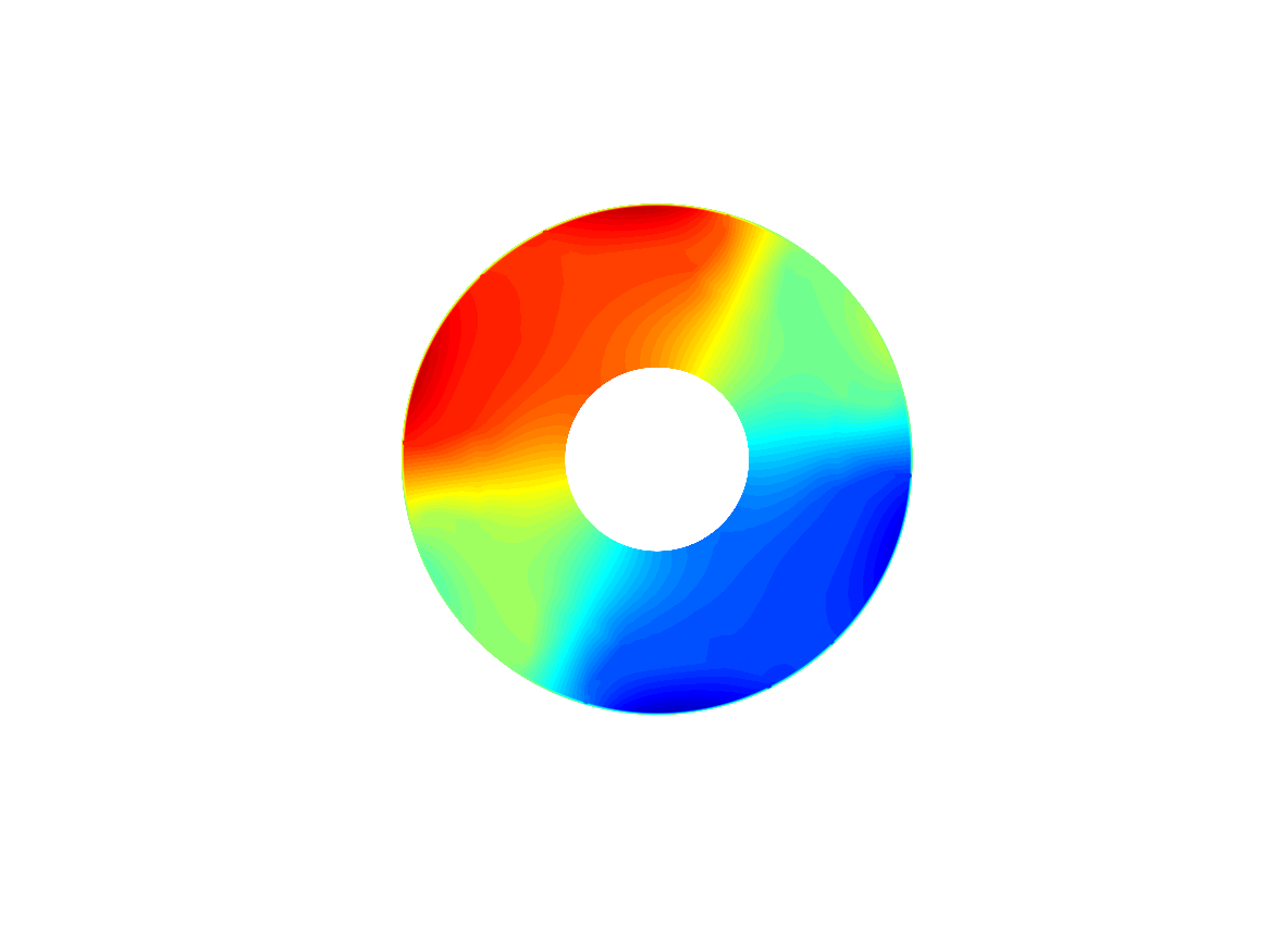 Figure 14
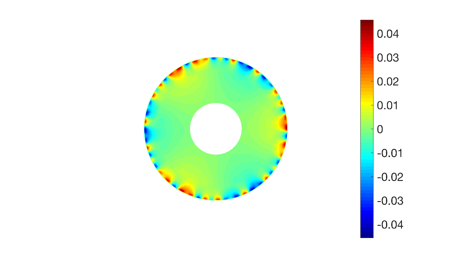 Figure 15
 Figure 16
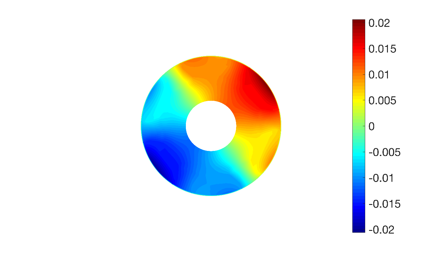 Figure 17
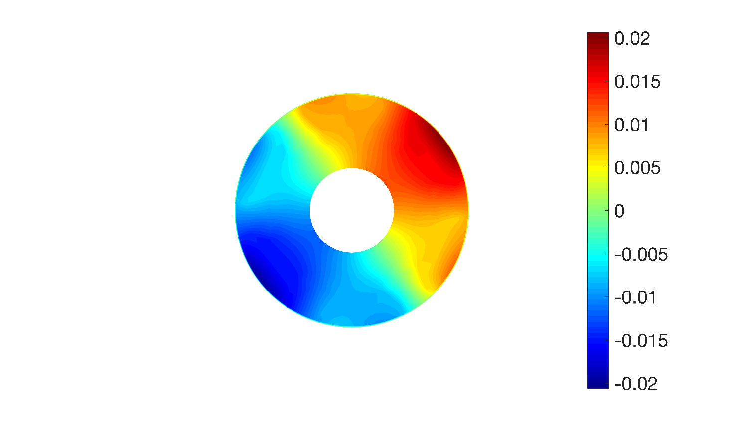 Figure 18
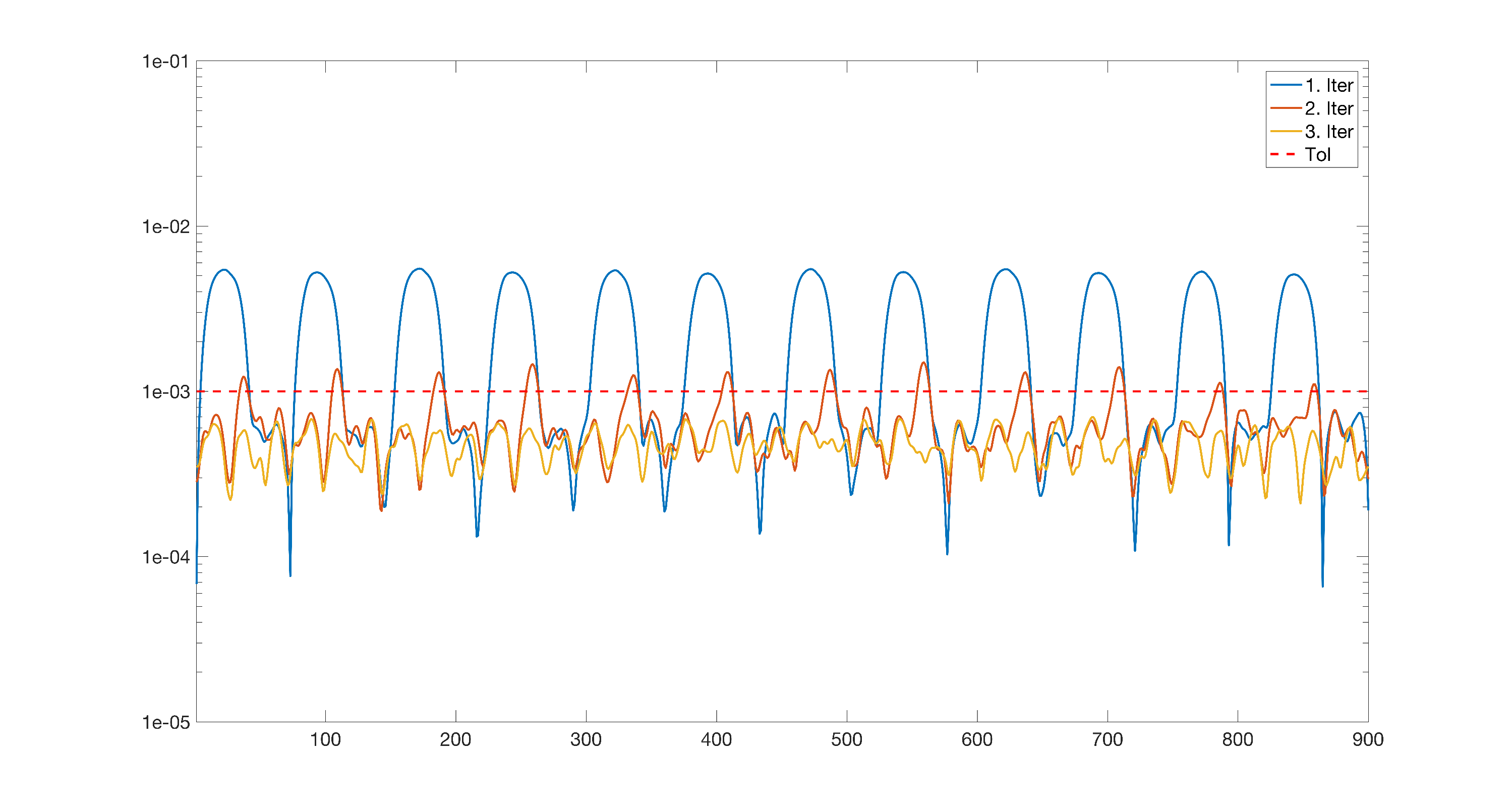 Figure 19
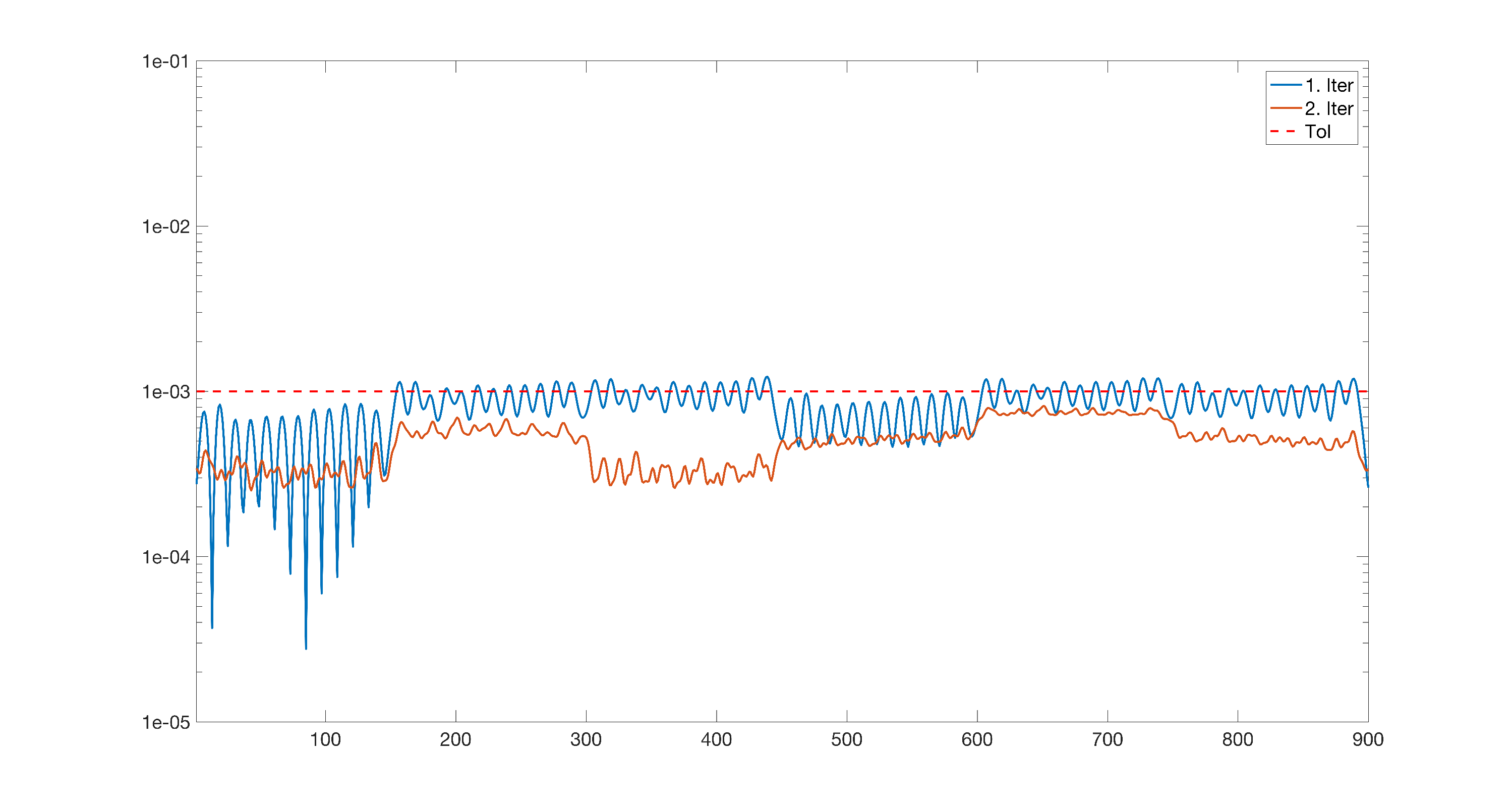 Figure 20
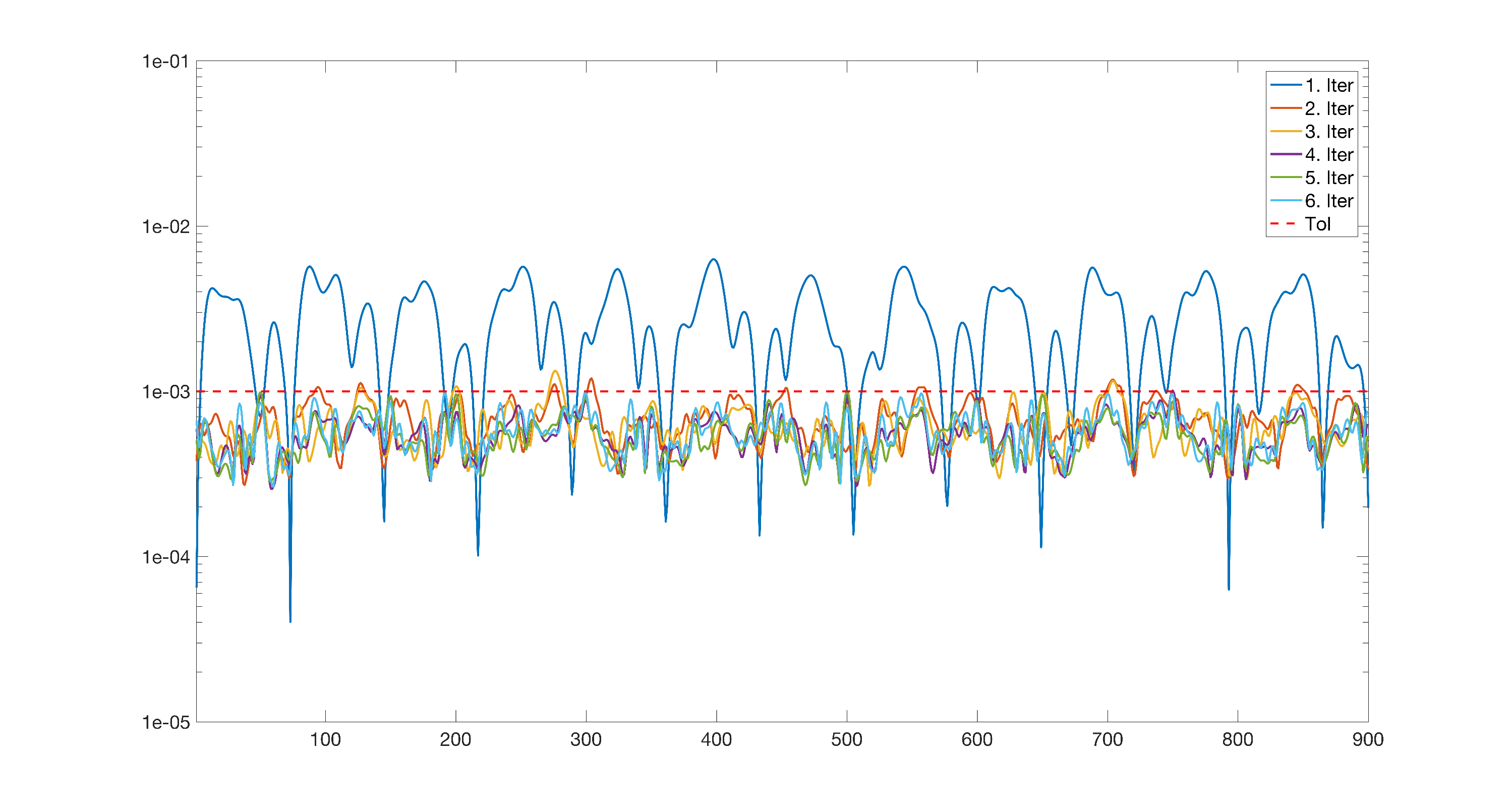 Figure 21
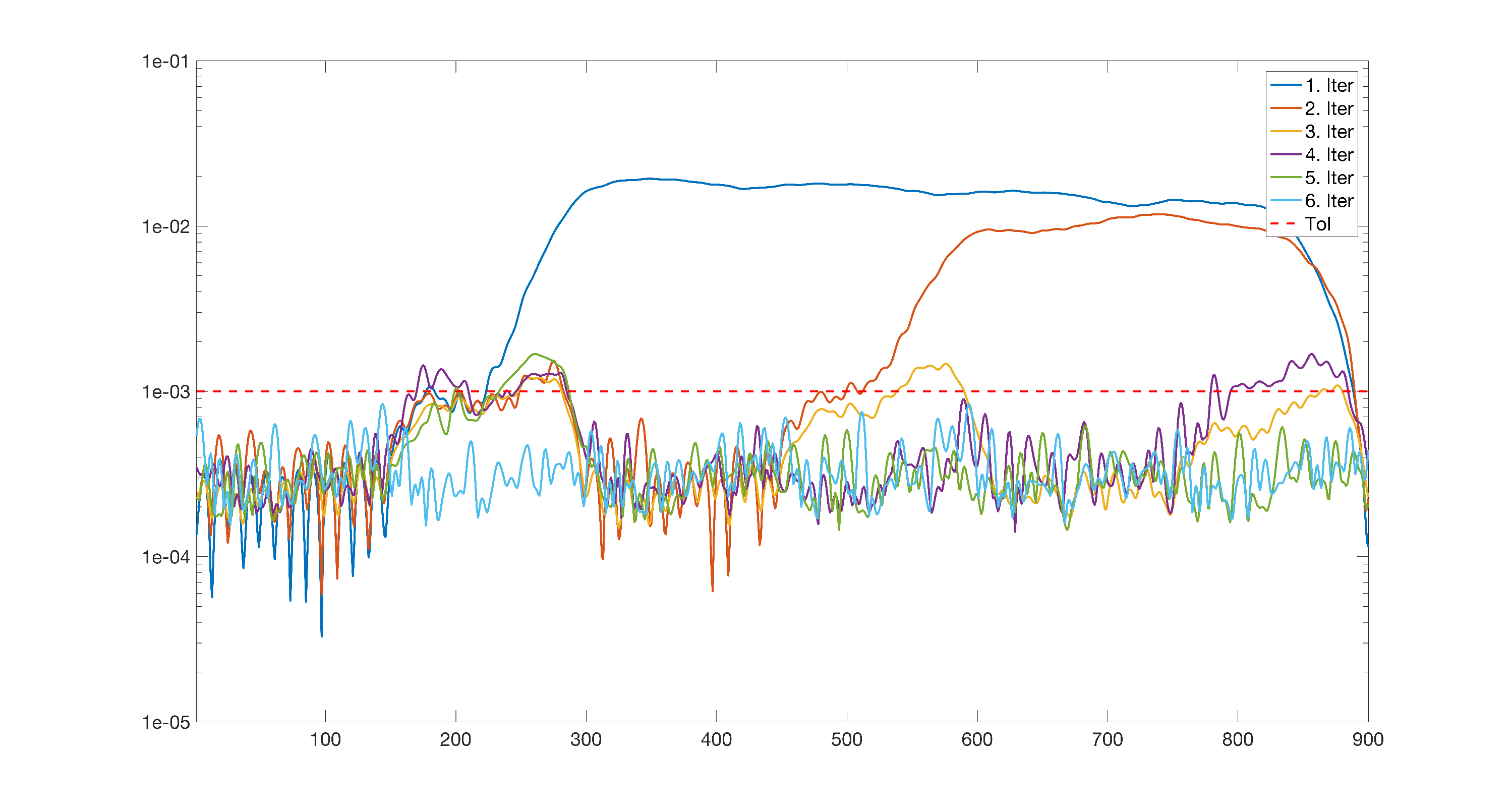 Figure 22
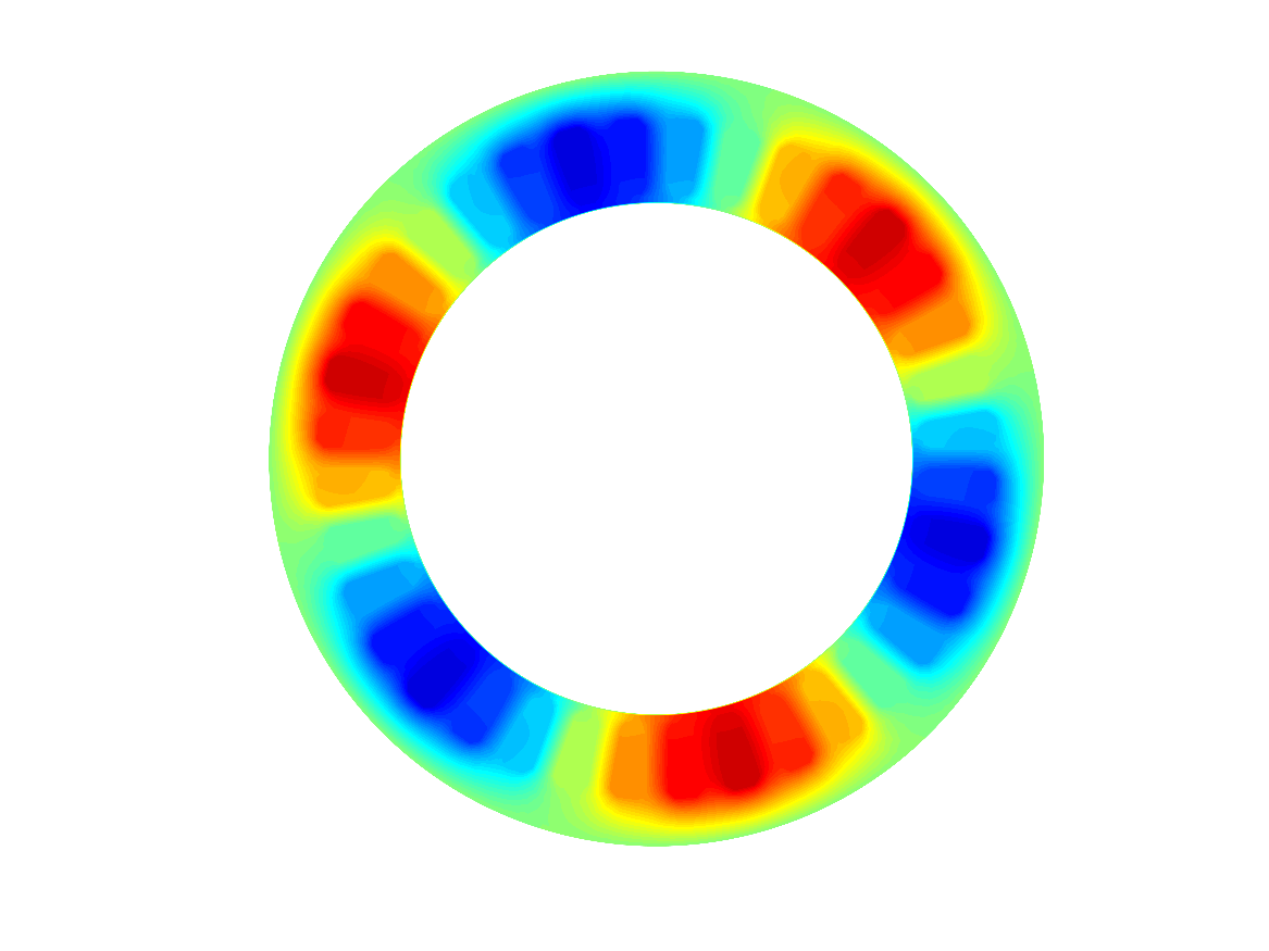 Figure 23
 Figure 24
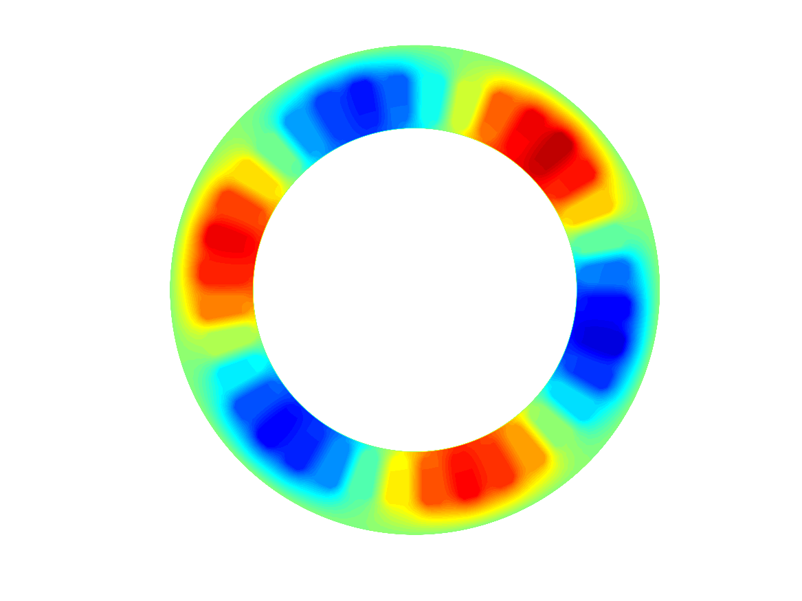 Figure 25
 Figure 26
 Figure 27
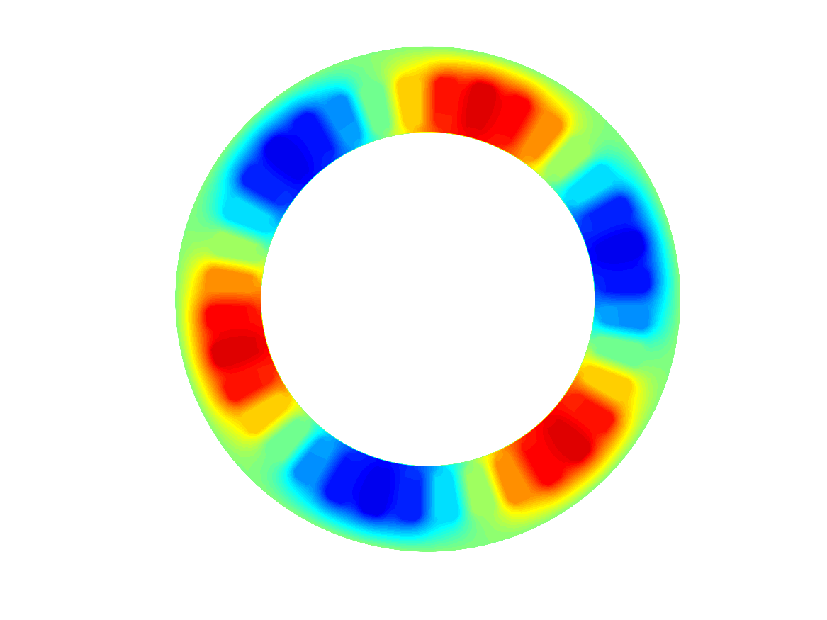 Figure 28
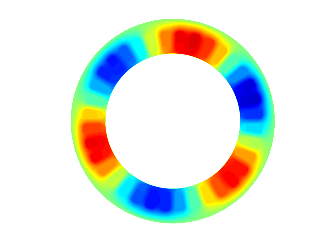 Figure 29
 Figure 30
 Figure 31
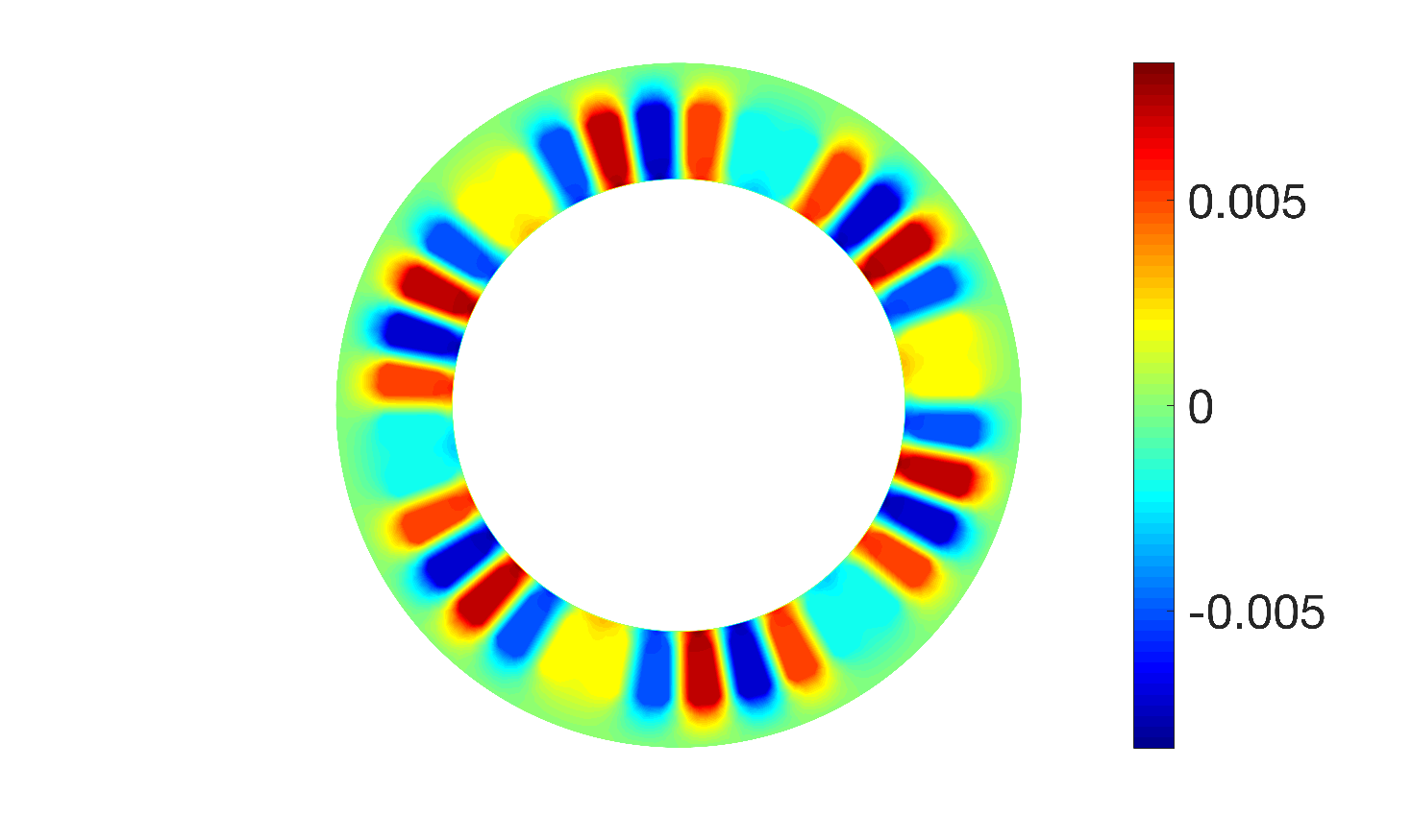 Figure 32
 Figure 33
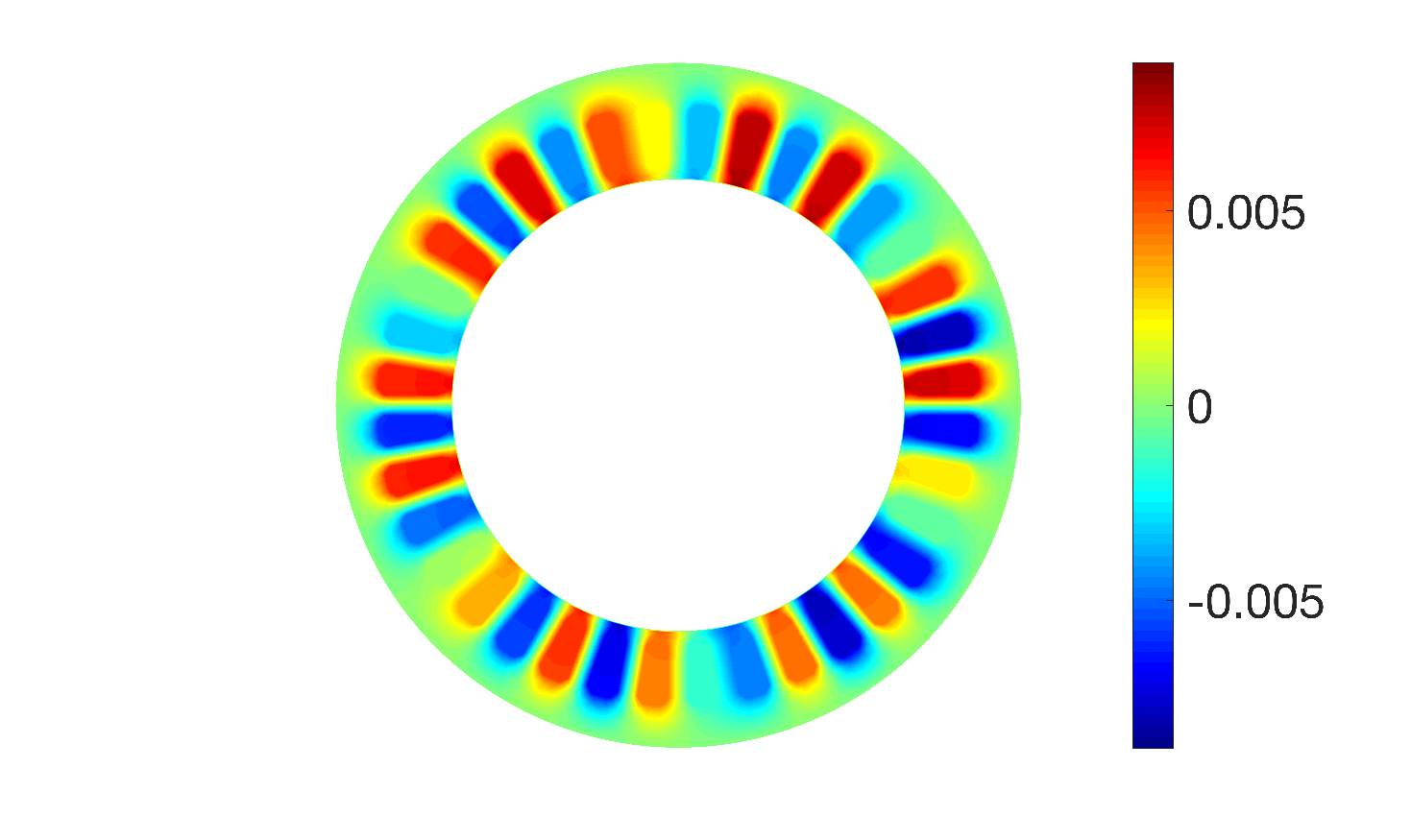 Figure 34
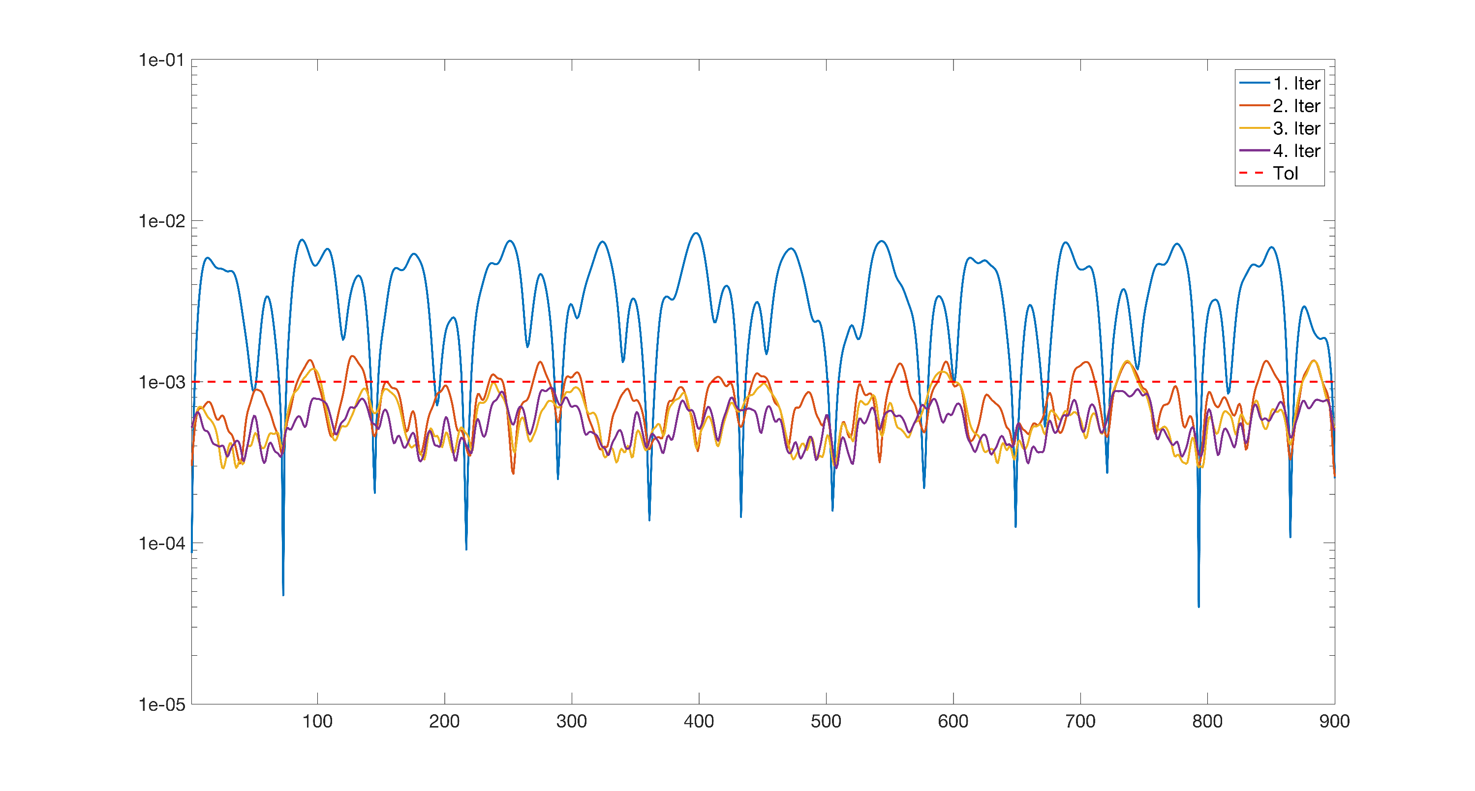 Figure 35
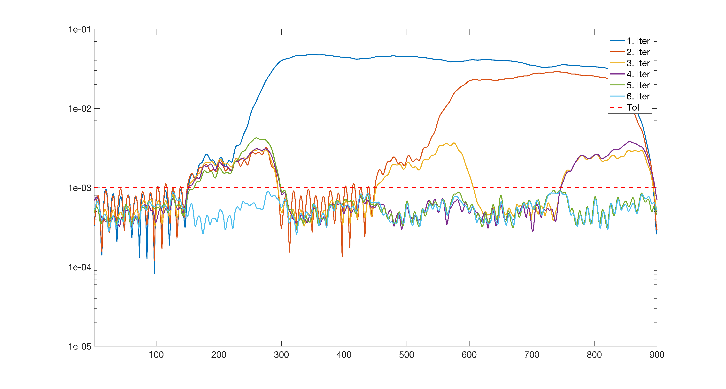 Figure 36
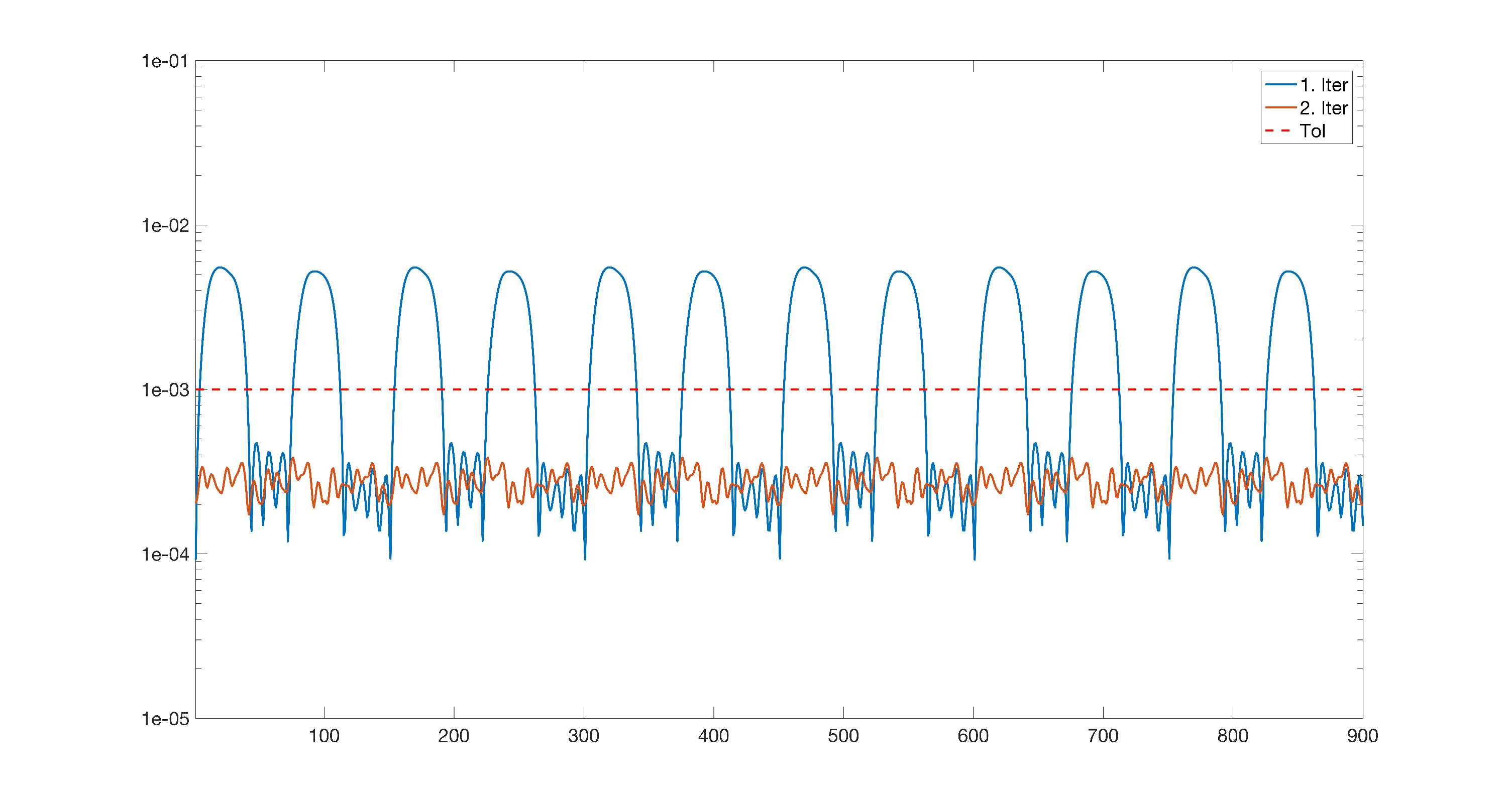 Figure 37
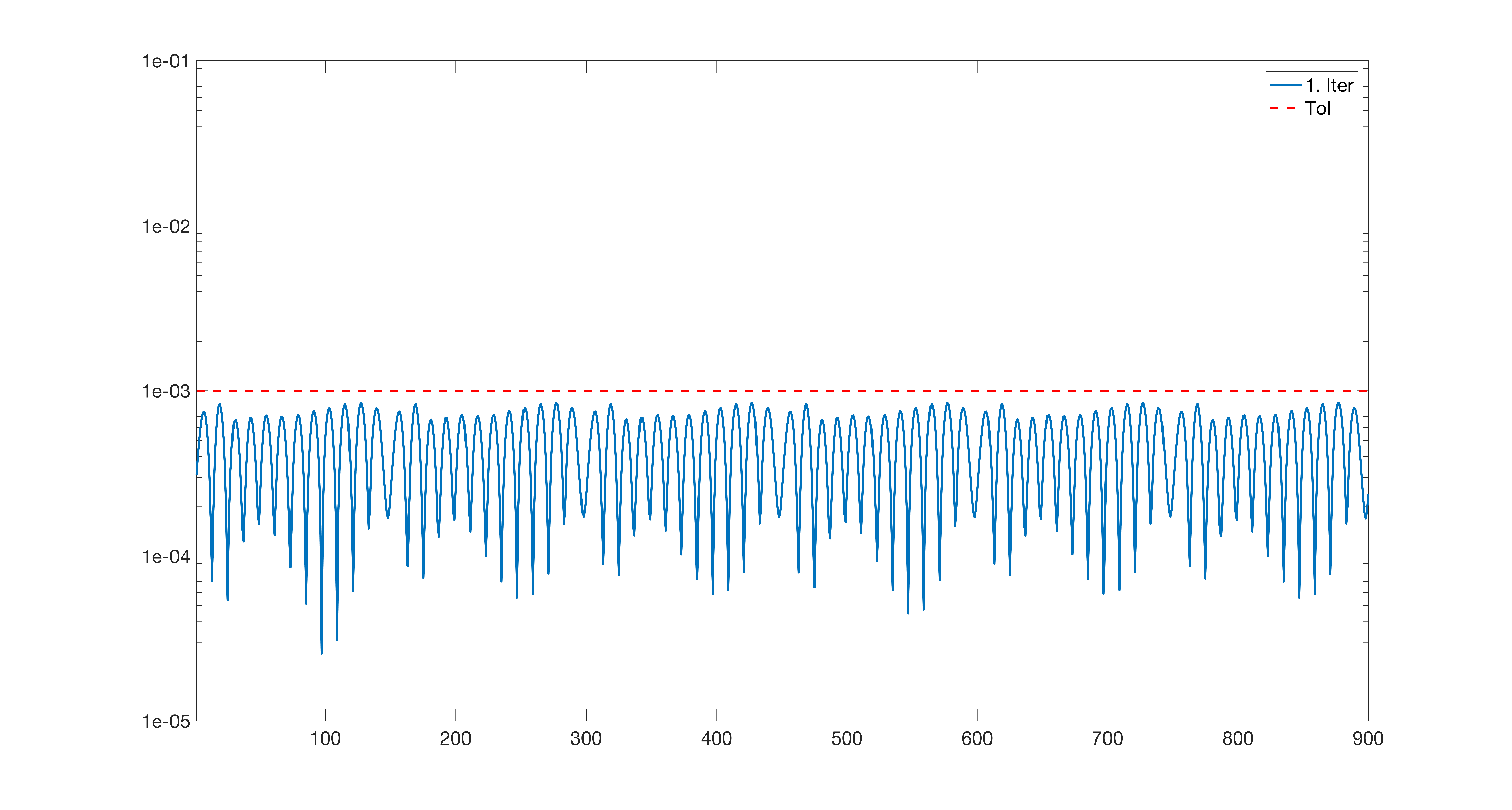 Figure 38
| Setting | FEM (sec.) | ROM (sec.) | Basis | Iter. | Speedup | Overhead |
| \svhline sym | % | |||||
| rot | % | |||||
| stat | % | |||||
| rot_stat | % |
| Setting | FEM (sec.) | ROM (sec.) | Basis | Iter. | Speedup | Overhead |
| \svhline sym | % | |||||
| rot | % | |||||
| stat | % | |||||
| rot_stat | % |
Peer Reviews
No public reviews on file for this paper yet. If you reviewed it on a platform where reviews are public (OpenReview, ICLR, NeurIPS, ICML), you can paste yours below so the community can read it here.
Videos
No videos yet. Explain this paper in a talk, walkthrough, or lecture? Add one.
Taxonomy
TopicsElectric Motor Design and Analysis · Model Reduction and Neural Networks · Hydraulic and Pneumatic Systems
11institutetext: Zeger Bontinck 22institutetext: Technische Universität Darmstadt, Graduate School of Computational Engineering, Dolivostr. 15, 64293 Darmstadt, Germany, 22email: [email protected] 33institutetext: Oliver Lass 44institutetext: Technische Universität Darmstadt, Department of Mathematics, Chair of Nonlinear Optimization, Dolivostr. 15, 64293 Darmstadt, Germany, 44email: [email protected] 55institutetext: Sebastian Schöps 66institutetext: Technische Universität Darmstadt, Graduate School of Computational Engineering, Dolivostr. 15, 64293 Darmstadt, Germany, 66email: [email protected] 77institutetext: Oliver Rain 88institutetext: Robert Bosch GmbH, 70049 Stuttgart, Germany, 88email: [email protected]
Model Order Reduction for Rotating Electrical Machines
Zeger Bontinck
Oliver Lass
Sebastian Schöps and Oliver Rain
Abstract
The simulation of electric rotating machines is both computationally expensive and memory intensive. To overcome these costs, model order reduction techniques can be applied. The focus of this contribution is especially on machines that contain non-symmetric components. These are usually introduced during the mass production process and are modeled by small perturbations in the geometry (e.g., eccentricity) or the material parameters. While model order reduction for symmetric machines is clear and does not need special treatment, the non-symmetric setting adds additional challenges. An adaptive strategy based on proper orthogonal decomposition is developed to overcome these difficulties. Equipped with an a posteriori error estimator the obtained solution is certified. Numerical examples are presented to demonstrate the effectiveness of the proposed method.
1 Introduction
Model order reduction for partial differential equations is a very active field in applied mathematics. When performing simulations in D or D using the finite element method (FEM) one arrives at large scale systems that have to be solved. Projection based model order reduction methods have shown to significantly reduce the computational complexity when applied carefully. While being applied to many different fields in physics, the application to rotating electrical machines is more recent HC14 ; LU16 ; MHCG16 ; SSSI16 . We will focus especially on the setting of non-symmetric machines. While the perfect machine is symmetric and simulations are usually carried out exploiting these properties, in real life the symmetry is often lost. This is due to perturbation in the geometry (e.g., eccentricity) and material properties and requires that the whole machine is simulated and not only a small portion (e.g., one pole). Hence this leads to an increase in the computational cost. The aim is to develop an adaptive strategy that is able to collect the required information systematically. Ideally, the algorithm is able to detect symmetries and exploits them if present. The greedy algorithm introduced in the context of the reduced basis method is a possible candidate PR06 ; QMN16 . A commonly used method in engineering and applied mathematics is the method of snapshots, or proper orthogonal decomposition (POD) Cha00 ; HLBR12 ; Sir87 . We opt for a combination of the two methodologies. The goal is a fast and efficient variant that avoids the necessity of an online-offline decomposition. This allows a broader application since no expensive offline costs have to be invested. Hence the method will already pay off after one simulation and not only in the many query context.
Additionally, the developed strategy has to be able to handle the motion of the rotor. While there are a number of methods to treat the rotation DRL85 ; PC95 ; SLDP06 , we will assume a constant rotational speed which allows us to utilize the locked step method PRS88 . Hence we can avoid the remeshing which is computationally prohibitive. Moreover, the application of other approaches should be straight forward.
Efficient simulation tools are a key ingredient when performing optimization or uncertainty quantification. The combination of model order reduction and optimization has caught a lot of attention DH15 ; GV17 ; NGMQ13 ; QGVW17 ; ZF15 . Especially in the many query context, where models have to be evaluated repeatedly and the need for accurate, fast and reliable reduced order models is high. While we will not look into the application of the reduced order models, we will develop a strategy that fulfills these needs. By using existing simulation tools in the adaptive procedure it is possible to insert the developed strategy into an existing framework and utilize the benefits of the reduced order model, as shown in LU16 .
The article is structured as follows: In Section 2 the permanent magnet synchronous machine (PMSM) is introduced. The discretization and the proposed model order reduction strategy are introduced in Section 3. Then in Section 4 numerical experiments are presented. Lastly, a conclusion is drawn in the last section.
2 Problem Description
The PMSM under investigation has six slots per pole and a double layered winding scheme with two slots per pole per phase. The geometry of the full machine is shown in Figure 1 (left) together with a detailed view on one pole (right). In each pole there is one buried permanent magnet indicated in gray. The machine has depth . It is operated at , resulting in a rotational speed of revolutions per minute (RPM). The machine is composed of laminated steel with a relative permeability .
In the following and refer to the stator and rotor domain, respectively. The whole domain is then referred to as and will be used for simpler notation when appropriate. Additionally, let us define the interface (dashed line) in the airgap between the rotor and the stator. Furthermore, we introduce the boundaries and of the stator and rotor, correspondingly. In the simulation we will account for the movement of the rotor, hence we introduce the angle that describes the position of the rotor with respect to the stator. For clarity we will append to the components related to the rotor.
To calculate magnetic vector potential of the machine, the magnetostatic approximation of the Maxwell’s equations has to be solved for both domains. This implies that the eddy and displacement currents are neglected and one obtains the semi-elliptic partial differential equations
[TABLE]
with Dirichlet boundary conditions on , with the outer unit normal. The reluctivity is depicted by a scalar since only linear isotropic materials are considered and nonlinearity is disregarded since a linearization at a working point is assumed. is the magnetic vector potential, represents the imposed source current density, which is related to the applied currents in the coils, and the remanence of the permanent magnets. The applied current density is aligned with the -direction, whereas the remanence is in the -plane. It is generally accepted that machines are adequately modeled in D, meaning that the magnetic field has no -component: . Since , one can write . Hence we end up with the linear elliptic equation
[TABLE]
where and are the -component of and , respectively. Further, the boundary conditions are given as previously introduced by on .
Let us next have a look at possible imperfections in the presented geometry and model. These are introduced during mass production of the PMSMs and are given by small deviations in the geometry or material properties. While there are many possible properties that can occur, we focus on two types. On the one hand we look at imperfection in the material of the permanent magnet, more precisely we consider deviations in the magnetic field angle of the permanent magnet OH13 . The second imperfection we consider is the length of the teeth in the stator Cle13 ; OMNCDH15 . Both quantities are depicted in Figure 1 (right). Perturbations in these quantities may lead to underperformance of the PMSM.
3 Model order reduction
In this section we discuss a method to accelerate the simulation of the PMSM. We will start by introducing the finite element discretization. Further, the realization of the rotation is outlined for the discrete setting. The resulting linear system of equations are of large scale and hence expensive to solve. In a next step we will present a model order reduction method based on proper orthogonal decomposition to speedup the simulations.
3.1 Finite element discretization
We obtain the discrete version of (2) by utilizing the finite element method (FEM). Discretizing by linear edge shape functions one makes the Ansatz
[TABLE]
where depicts the nodal finite elements which are associated with the triangulation of the machine’s cross-section and is the unit vector in -direction. Using the Ritz-Galerkin approach, the -dimensional linear discrete system
[TABLE]
is obtained, where are the finite element system matrices, depict the degrees of freedom (DoFs) and the discretized versions of the current densities and permanent magnets.
To take the motion of the rotor into account in the simulation, we utilize the locked step method PRS88 ; SLDP06 . For the implementation, a contour in the airgap is defined () which splits the full domain into two parts: a fixed outer domain connected to the stator and an inner domain connected to the rotor , where the mesh will be rotated. At the contour the nodes are distributed equidistantly. The angular increments are chosen so that the mesh of the stator and rotor will match on the interface. The nodes on the interface are then reconnected leading to the mesh for the next computation. Using this technique, the rotation angle is given by with . We can hence partition the discrete unknown in into a static part, a rotating part and the interface, with dimensions , and , respectively. This idea is a particularization of non-overlapping domain decomposition AHH11 ; TW05 . The linear system (3) can then be written as
[TABLE]
where , , and are the stiffness matrices and right hand sides on the static and moving part and do no longer depend on the angle . For the points on the interface there are two cases. The interface of the static part is independent of the angle and hence we get the corresponding stiffness matrix . For the rotor side we have to perform the shift, this is indicated with in the corresponding stiffness matrix . On the interface also a shift has to be performed hence also here the corresponding stiffness matrix and right hand side are dependent on . Let us note that it is not required to reassemble matrices. All of these shifts can be performed by index shift and hence allow a very efficient implementation. The size of the system does not change, i.e., we have .
For completeness let us remark on the domain deformation introduced by . Since we are in the setting of a parametrized shape transformation, i.e., one for each tooth in the stator we can utilize an affine geometry preconditioning to describe the transformation. This allows to carry out the computation on a reference domain and hence avoids again expensive remeshing and its undesired consequences as e.g., mesh noise. The stiffness matrices and right hand sides can be written in the form
[TABLE]
where and are local matrices. For a detailed description including computational procedures, we refer the reader to RHP08 .
3.2 Proper orthogonal decomposition
The goal is to generate a reduced order model to accelerate the simulation of (4). The simulation of the rotation is computationally expensive since the discretization of (2) leads to very large linear systems that need to be solved for every angular position. While in symmetric machines this can be avoided, in the case of non-symmetric machines a whole revolution has to be simulated. Hence we require an efficient strategy to overcome this problem. For this we investigate an adaptive strategy that builds a surrogate model while performing the simulation and switches to it when the required accuracy is reached. We want to use information collected over the rotational angle and generate a projection based reduced order model. In the past, model order reduction methods based on proper orthogonal decomposition (POD) Cha00 ; HLBR12 ; KV01 , balanced truncation AHH11 ; HSS08 and the reduced basis method PR06 ; QMN16 ; RHP08 have been developed to speedup the computation. More recently, the POD method has been successfully applied to rotating machines HC14 ; LU16 ; MHCG16 ; SSSI16 . In this work we consider a combination of POD and the reduced basis method. We will not pursue an online-offline decomposition but rather see the reduced order model as an accelerator for the simulation.
Let us start by recalling the POD method so we can develop an extension suitable for the application presented. Let the solution to (2) be given in the discrete form, i.e., let be the solution to (3) for a fixed angle . The snapshots are then given by for , where is an index set with elements in for which (3) is solved. A POD basis is then computed from these snapshots by solving the following optimization problem:
[TABLE]
where stands for the weighted inner product in with a positive definite, symmetric matrix . The goal is to minimize the mean projection error of the given snapshots projected onto the subspace spanned by the POD basis . By introducing the matrix as the collection of the snapshots with we can write the operator arising from the optimization problem (5) as
[TABLE]
Then the unique solution to (5) is given by the eigenvectors corresponding to the largest eigenvalues of , i.e., with GV17 . The operator is largesince it is of dimension which we want to reduce. Hence it might be better in many cases to set up and solve the eigenvalue problem
[TABLE]
and obtain the POD basis by . Note that both approach are equivalent and are related by the singular value decomposition (SVD) of the matrix . While the latter is computationally more efficient, the singular value decomposition is numerically more stable. A comparison of the different computations was carried out in LV13 . For completeness let us state the POD approximation error given by
[TABLE]
where is the rank of . For easier notation we collect the POD basis in the matrix .
After introducing the computation of the POD basis we will now outline the adaptive approach utilized in this work. It is crucial to minimize the number of solves involving the FEM discretization in order to obtain a speedup of the computation. The goal is to push most of the computations in the simulation onto the reduced order models. However, we have to guarantee that the reduced order models are accurate in order to obtain reliable results. We will present a strategy that does not require precomputation as for example in the reduced basis method but performs the model order reduction during the simulation. First let us outline how the POD basis is applied to (4). In the second step we give the details on how to obtain the basis efficiently.
We generate for each part of the machine an individual POD basis. Hence we have one basis for the stator and one basis for the rotor. The interface between the stator and the rotor is not reduced, i.e., we work with the FEM ansatz space on the interface. This is motivated by the observation that the decay of the eigenvalues on is very slow, which would result in a large POD basis. Since the FEM space for the interface is usually of moderate dimension, the gain of using POD would be negligible. We compute the POD basis as solution to (5) utilizing the snapshots and to obtain and , respectively. We then make the ansatz
[TABLE]
where the POD coefficients are indicated with a bar. By projecting (4) onto the subspace spanned by the POD basis, we obtain the reduced order model
[TABLE]
In short notation the system will be written as
[TABLE]
with the vector of POD coefficients. This system is of dimension and of much smaller dimension as the original system (4) which was of dimension .
Next we introduce the strategy on how to determine the POD basis adaptively. The goal is to reduce the computational cost with respect to the rotation. A full revolution requires solves of the system (4), i.e., for all with . In the symmetric case it is not required to solve a full rotation but only for angles that cover one pole, for our particular example this means one sixth, i.e., solutions are needed. Note, we assume that is divisible by , where is the number of poles of the machine. In the non-symmetric case this is not possible. The idea is to generate a sequence of disjoint sets with . Note that the sets can also be chosen arbitrarily as long as they fulfill the subset property. This is required to be able to reuse the already computed snapshots and hence minimize computational overhead. Ideally the sets are not too large but are large enough to cover the most important features. The strategy is then as follows: We start by choosing and evaluate (4) for and . From the computed solutions/snapshots a POD basis is computed. Then an error estimator , , is evaluated to determine the maximum error. If the error is larger than a given tolerance the index is determined where the maximum error is attained. Determine the set that contains the index and the snapshot set is enlarged by adding the new solutions corresponding to to the old ones, i.e., . This procedure is repeated until the error , , is below the desired threshold. For stability reasons the sets that have been already used are removed from the list. In this case the index for the second largest error is used. During the numerical experiments this scenario never occurred and hence will not be investigated further. In Algorithm 1 the strategy is summarized. This sampling of the sets is similar to the greedy algorithm from the reduced basis method. The decision to add more than one solution at a time to the snapshot set is to minimize the overhead of evaluating the error estimator and generating the reduced order models. Since we do not introduce an online-offline decomposition the computations of error estimator and the generation of the reduced order models are included in the computational costs. In our numerical tests the proposed strategy converges very fast, in at most iterations. Depending on the asymmetry different sets may preform better. This will be illustrated with numerical experiments. For the symmetric case we observe that usually only one set is visited (if chosen appropriately). In other words: the symmetry is correctly detected by the algorithm. In Section 4 the specific choices of the sets are described and a comparison of different strategies is performed. The dimension of the computation of the POD basis is chosen such that
[TABLE]
holds for the stator and rotor independently. This is a popular choice, where a typical value is . Note that the denominator can be computed by and hence not all eigenvalues have to be computed.
Let us now shortly have a look at the error estimator. For this let us recall some basic quantities. We define the discrete coercivity constant by
[TABLE]
Hence the the coercivity constant is given by the smallest eigenvalue such that
[TABLE]
is satisfied for and QMN16 . Further, we define the residual . Then the error introduced by the reduced order model in the variable can be characterized by
[TABLE]
Additionally, we look at the relative error which might be more interesting in many applications. The corresponding error estimator reads
[TABLE]
This is a standard result and can be found in PR06 ; RHP08 . In the numerical realization we set the weight matrix to the dimensional identity matrix. Other choices (e.g., ) are possible but not investigated at this point. Note that the rotation as introduced in this work does not influence the coercivity constant and hence the dependence can be omitted. This can also be seen in the numerics, where only small deviations can be observed which are in the order of discretization. Hence a very efficient realization is possible, since only one eigenvalue problem has to be solved. Let us remark that the error is measured with respect to the finite element solution. It is assumed that the finite element solution is accurate enough to approximate the solution of the continuous problem. Let us remark that the computation of the residual norms can be performed very efficiently using the introduced affine decomposition DH15 .
4 Numerical results
We will now present different numerical results. For this let us specify the settings. The geometry (Figure 1) is discretized using a triangular mesh with nodes and the interface is discretized by equidistant points. Hence one revolution requires the linear system (3) to be solved times. Here is where model order reduction will come into play and speedup the simulation significantly. All computation are performed on a standard desktop PC using Matlab R2016b. Throughout our numerical tests we will consider three settings:
sym
Symmetric machine.
rot
Perturbation of in one permanent magnet by .
stat
Perturbation of in one tooth by mm.
rot_stat
Perturbation in both and .
To start we will have a look at the performance of the POD method. For this we compute a full revolution for each of the four setting and have a look at the decay of the eigenvalues. Let us recall that a fast decay is essential for the POD method to perform well. In Figure 2 the decay of the normalized eigenvalues is shown. As can be seen the eigenvalues decay very fast for rotor and stator. Only for the interface the decay is much slower. This underlines the decision to not perform a model order reduction for the interface. Additionally it can be observed that a perturbation in the magnetic field angle has less influence on the decay of the eigenvalues than the perturbation in the length of one stator tooth. While the perturbation in causes a slight change in the decay of the eigenvalues related to the stator, the perturbation in dramatically influences the eigenvalues related to the rotor.
Next we depict the first three POD basis vectors for each setting (Figure 3-6). For the setting sym and rot very similar basis vectors are obtained. The last basis vector for both settings is zero on wide areas and only adds contributions at the interface (green is zero). In the settings stat and rot_stat this is very different. There the third basis vector for the rotor still contributes a lot of information to the reduced order model. What was already observed in the decay of the eigenvalues was verified again in the POD basis vectors. The settings sym and rot exhibit similar behaviors as well as stat and rot_stat.
From the decay of the eigenvalues it can be expected that we will be able to generate reduced order models of very low dimension. The plots of POD basis verify this for the sym and rot since already the third basis vector is almost zero.
Next we have a look at the performance of the presented adaptive algorithm. For this let us introduce the index sets . We will look at two settings. To be able to differentiate the two settings we will call sets and . In the first we choose the sets by dividing the full rotation into six sections (6 poles). within each section we have a hierarchy of sets for refinement. Hence the sets can be written as follows
[TABLE]
Note that the values for are always less than . Using these sets we always compute snapshots only related to one pole. If the error is still to large in the particular pole a refinement is achieved.
In the second setting distributed index sets are considered. This allows for a broader information collection since the snapshots are immediately distributed over the whole range of . We define the corresponding sets by
[TABLE]
With these particular choices we get in both settings sets with each indices and hence we can perform a fair comparison of the two approaches. In our experiment it turned out that these settings are a good trade between performance and accuracy. As the tolerance for our adaptive strategy we use which is sufficient for most applications. The error estimator overestimated the real error by at most one order of magnitude. This is a good result since it guarantees that the model is not refined unnecessarily often.
The results for the two different index sets and are shown in Figure 7-8. We plot the relative error of the angular position for every iteration of the adaptive algorithm. The actual error is omitted in the plots for visual clarity. By a dashed line the tolerance is indicated as a visual aide. It can be seen how each of the two index sets have very different behaviors.
The set , which uses a kind of local refinement of the snapshots, performs well for the sym and rot. In the behaviour of the error it can be clearly seen in which region new snapshots were added. The error of the region drops significantly. As was expected, the symmetric case only requires one iteration since already a few snapshots contain enough information to compute the full rotation. For the perturbation in the rotor a second set of snapshots is required to push the error below the tolerance . A clear accuracy difference between the poles can be observed which is reflected by steps in the error. The settings stat and rot_stat are not handled too well by the local nature of the set . For each pole a snapshot set is selected resulting in six iterations for both settings.
On the other hand the index set shows the advantages of the global nature of the snapshot selection. While for sym and rot this results in more iterations as for the set in the other two settings, the benefits can be observed. In particular for stat, a much faster convergence of the adaptive algorithm is obtained. The error also has a different nature. In each iteration the error is reduced uniformly over the whole rotation and not only locally.
Next we have a look at the performance of the adaptive algorithm. For this we compare computational time (wall clock time) of the different approaches. The computational time is determined by the average over runs to flatten out irregularities in the numerical realization. Note that the mesh and the constant finite element matrices are precomputed, and hence are not reflected in the run time. This does not influence the result since it is required by both approaches and gives a more clear indication of the computational costs, which is the main focus. In Table 4-4 the results are summarized.
The reference list from the paper itself. Each links out to its DOI / PubMed record.
- 1(1) Antil, H., Heinkenschloss, M., Hoppe, R.H.W.: Domain decomposition and balanced truncation model reduction for shape optimization of the Stokes system. Optim. Method Softw. 26 (4-5), 643–669 (2011)
- 2(2) Chatterjee, A.: An introduction to the proper orthogonal decomposition. Current Science 78 , 539–575 (2000)
- 3(3) Clénet, S.: Uncertainty quantification in computational electromagnetics: The stochastic approach. ICS Newsletter. 20 (1), 2–12 (2013)
- 4(4) Davat, B., Ren, Z. and Lajoie-Mazenc, M.: The movement in field modelling. IEEE Trans. Mag. 21 (6), 2296–2298 (1985)
- 5(5) Dihlmann, M., Haasdonk, B.: Certified PDE-constrained parameter optimization using reduced basis surrogate models for evolution problems. Comput. Optim. Appl. 60 , 753–787 (2015)
- 6(6) Gubisch, M., Volkwein, S.: Proper orthogonal decomposition for linear-quadratic optimal control. In: Benner, P., Cohen, A., Ohlberger, M., Willcox, K. (eds.) Model Reduction and Approximation: Theory and Algorithms, To appear (2017)
- 7(7) Henneron, T., Clénet, S.: Model order reduction applied to the numerical study of electrical motor based on POD method taking into account rotation movement. Int. J. Numer. Model. 27 (3), 1099–1204 (2014)
- 8(8) Holmes, P., Lumley, J.L., Berkooz, G., Rowley, C.W.: Turbulence, Coherent Structures, Dynamical Systems and Symmetry. Cambridge University Press, Cambridge (2012)