Quantum theory of curvature and synchro-curvature radiation in a strong and curved magnetic field, and applications to neutron star magnetospheres
Guillaume Voisin (LUTH), Silvano Bonazzola (LUTH), Fabrice Mottez, (CNRS, LUTH)

TL;DR
This paper develops a quantum theoretical framework for curvature and synchro-curvature radiation in strong, curved magnetic fields, with applications to neutron star magnetospheres, bridging classical and quantum descriptions of particle radiation.
Contribution
It extends previous work by deriving quantum radiation from Dirac particles in curved magnetic fields, introducing discrete transitions and quantum recoil corrections.
Findings
Classical curvature radiation is recovered within the quantum framework.
Quantum synchro-curvature radiation expressions are derived.
Quantum recoil and deconfinement corrections are formulated.
Abstract
In a previous paper, we derived the quantum states of a Dirac particle in a circular, intense magnetic field in the limit of low momentum perpendicular to the field with the purpose of giving a quantum description of the trajectory of an electron, or a positron, in a typical pulsar or magnetar magnetosphere. Here we continue this work by computing the radiation resulting from transitions between these states. This leads to derive from first principles a quantum theory of the so-called curvature and synchro-curvature radiations relevant for rotating neutron-star magnetospheres. We find that, within the approximation of an infinitely confined wave-function around the magnetic field and in the continuous energy-level limit, classical curvature radiation can be recovered in a fully consistent way. Further we introduce discrete transitions to account for the change of momentum perpendicular…
Click any figure to enlarge with its caption.
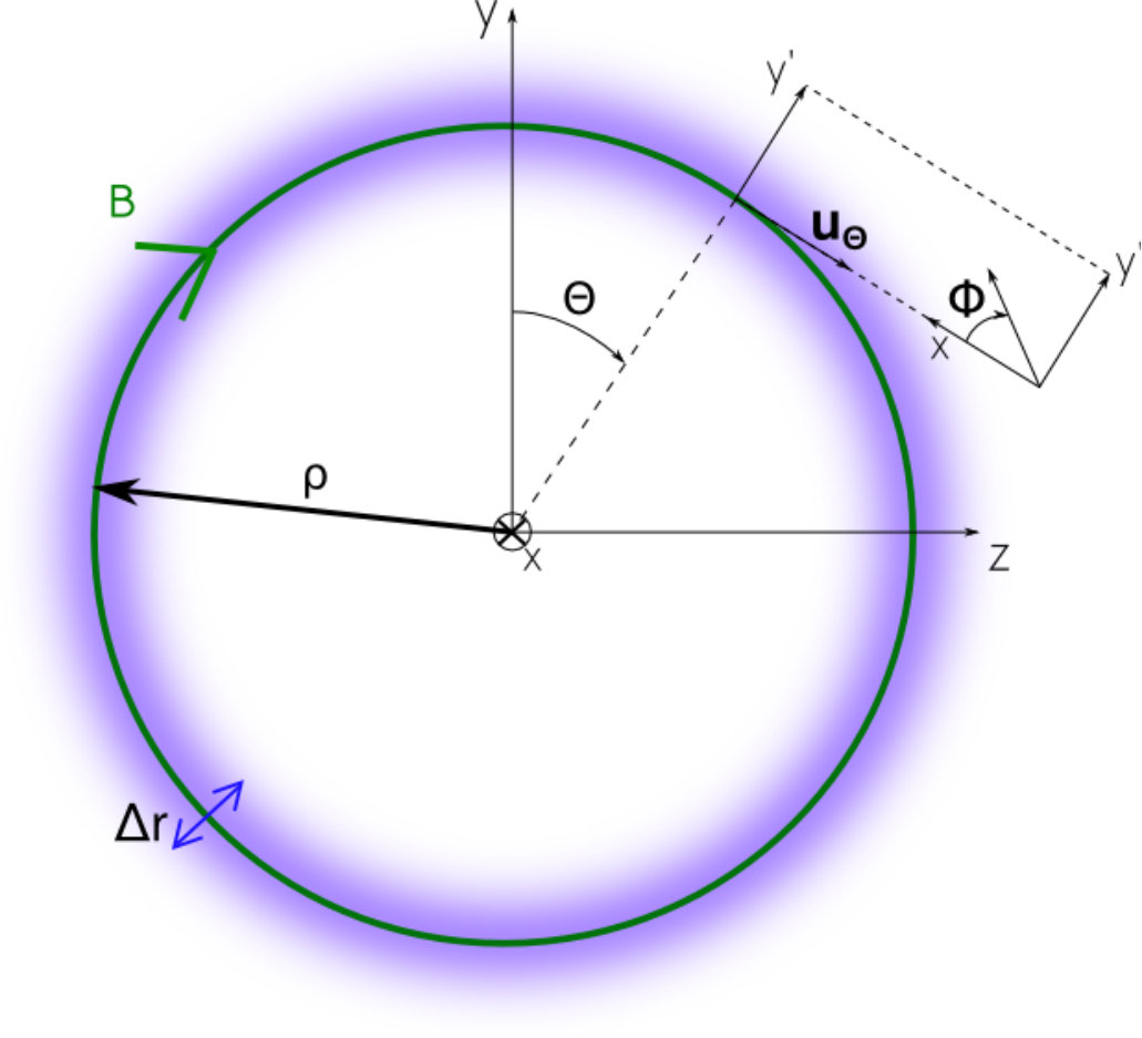 Figure 1
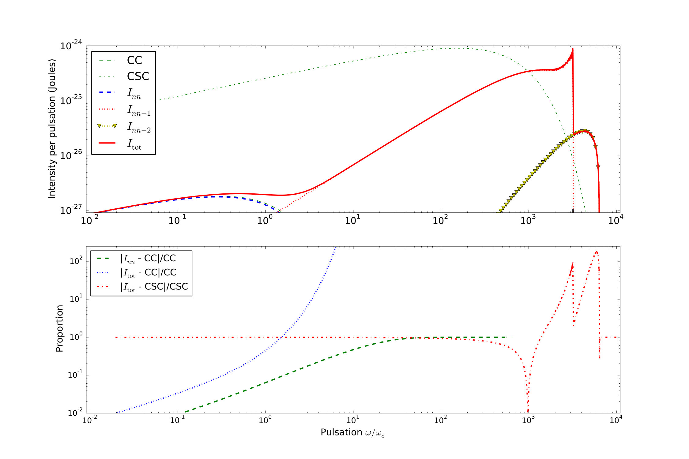 Figure 2
Peer Reviews
No public reviews on file for this paper yet. If you reviewed it on a platform where reviews are public (OpenReview, ICLR, NeurIPS, ICML), you can paste yours below so the community can read it here.
Videos
No videos yet. Explain this paper in a talk, walkthrough, or lecture? Add one.
Quantum theory of curvature and synchro-curvature radiation in a strong and curved magnetic field, and applications to neutron star magnetospheres
Guillaume Voisin
Silvano Bonazzola
LUTh, Observatoire de Paris, PSL Research University, 5 place Jules Janssen, 92190 Meudon, France
Fabrice Mottez
LUTh, Observatoire de Paris, PSL Research University - CNRS, 5 place Jules Janssen, 92190 Meudon, France
Abstract
In a previous paper, we derived the quantum states of a Dirac particle in a circular, intense magnetic field in the limit of low momentum perpendicular to the field with the purpose of giving a quantum description of the trajectory of an electron, or a positron, in a typical pulsar or magnetar magnetosphere.
Here we continue this work by computing the radiation resulting from transitions between these states. This leads to derive from first principles a quantum theory of the so-called curvature and synchro-curvature radiations relevant for rotating neutron-star magnetospheres.
We find that, within the approximation of an infinitely confined wave-function around the magnetic field and in the continuous energy-level limit, classical curvature radiation can be recovered in a fully consistent way. Further we introduce discrete transitions to account for the change of momentum perpendicular to the field and derive expressions for what we call quantum synchro-curvature radiation. Additionally, we express deconfinement and quantum recoil corrections.
pacs:
I Introduction
In a previous paper Voisin et al. (2017) (hereafter paper 1), we derived the states of an electron in a curved strong magnetic field within the approximation of a very low momentum perpendicular to the magnetic field. To ease calculations, it is convenient to consider a ”circular” magnetic field, that is the field lines are of constant curvature and so form circles. In this paper, we compute the transition rates between these states in the limit of high momentum parallel to the magnetic field, in such a way that parallel transition can be considered approximately continuous. Our goal is to derive a quantum-electrodynamics theory of curvature radiation and low synchro-curvature radiation in the context of rotating-neutron-star magnetospheres. These magnetospheres are characterized by intense magnetic field from Teslas for recycled millisecond pulsars to Teslas for magnetars. The radius of curvature of magnetic field lines is typically larger than km, which is the typical radius of the star, within the assumption of a dipolar magnetic field. Extremely large electric-potential gaps along the open magnetic-field lines ( see e.g. Arons (2009) for a review) accelerate charged particles to energies only limited by radiation reaction at Lorentz factors as high as .
In this regime, an electron looses all of its momentum perpendicular to the magnetic field after traveling a few meters in the synchro-curvature regime (see hereafter and Voisin et al. (2016a)). When only parallel momentum remains, radiation reaction is attributed to the so-called curvature radiation along the magnetic field Ruderman and Sutherland (1975), which is the radiation of a charged particle following exactly a locally circular trajectory. Synchrotron radiation can be seen as a particular case where the trajectory is the cyclotron trajectory. However, curvature radiation usually refers to the case of a magnetic-field-line trajectory, and therefore is not strictly physical, in the sense that a particle not rotating around the field does not undergo any force capable of keeping it along. Therefore, curvature radiation is better seen as the mathematical zero-perpendicular-momentum limit of the so-called synchro-curvature radiation Cheng and Zhang (1996) that describes the classical theory of radiation by a charged particle with low perpendicular momentum in a locally circular magnetic field. Quantum corrections where added by Zhang and Yuan (1998) and latter by Harko and Cheng (2002) in the form of an effective correction to classical expressions in analogy with equivalent photon theories developed for synchrotron radiation which essentially amounts to the replacement in the transition probability accounting or quantum recoil, where is the intensity per pulsation and is the energy of the particle. A formalism based on effective electric fields was developed Harko and Cheng (2002) to deal with further inhomogeneities of the magnetic field such as a perpendicular gradient of intensity. A more compact but equivalent formalism for synchro-curvature radiation was also developed Viganò et al. (2014). Recently, a description Kelner et al. (2015) with a self-consistent trajectory that takes carefully into account the drift along the cylinder generated by the circular field showed that the drift effectively changes the curvature radius for relatively large Lorentz factors or low magnetic field intensities. As we pointed out in paper 1, classical synchro-curvature radiation results in numerous cases in a very fast decay of the perpendicular momentum of the particle which can reach the first Landau levels, if one assumes the well-known quantum theory of an electron in a homogeneous-intensity uniform-orientation magnetic field (see e.g. Sokolov and Ternov (1968)). One then has to take into account discrete transitions from a Landau level to another Latal (1986), Harding and Preece (1987). This is particularly interesting when the plasma is at rest in the frame of the star such that the uniform-magnetic-field theory is locally relevant. This is the case for example in X-ray binaries where X-ray cyclotron lines have been observed and where two levels are typically separated by keV with Caballero and Wilms (2012).
Therefore, classical synchro-curvature cannot hold for very low perpendicular momenta since the synchrotron part becomes discrete. This effect cannot be taken into account with the usual quantum recoil corrections which apply in the continuous limit. Besides it does not take into account the fact that two quantum numbers are changing, one for parallel and another for perpendicular momenta. Simultaneously, cyclotron transitions are irrelevant for particles with high parallel momenta since they do not take into account longitudinal transitions, that is the curvature part of the radiation. In this paper, we start from first principles using the quantum states derived in paper 1. The resulting radiation results from transitions in the continuous approximation for parallel momentum variations and discrete for perpendicular momentum variations. Parallel transitions are treated in a similar way as Sokolov and Ternov (1968) did for the quantum theory of synchrotron radiation (see also Schwinger (1954) and Schwinger and Tsai (1978)). With this formalism syncho-curvature-like and curvature-like components appear in a very distinct fashion. As mentioned in paper 1, we neglect every drift of the particle, which is very appropriate except at extremes of the magnetic-field and Lorentz-factor ranges mentioned above. We also find additional corrections in where are positive integers, Teslas the critical field of Landau states and the magnetic-field intensity. We interpret these as deconfinement corrections, in the sense that they give the difference between a point-like particle and an extended wave-function around the magnetic-field line. At leading order, we find the classical curvature radiation.
This paper is organized as follow: in section II we introduce the general formalism to compute quantum transitions, in section III we develop this formalism in the particular case of curvature radiation which allows us to introduce notations and concepts that we generalize in section IV to the general case of synchro-curvature radiation, in section V we integrate the previously found expressions over solid angles to obtain power spectra and in section VI we discuss these results around the example of a millisecond pulsar.
II Radiation of a confined particles in quantum electrodynamics
We compute the interaction of the electron with the photon vacuum to the first order of perturbation theory. The Hamiltonian of interaction is
[TABLE]
where is the initial state of the electron, the Dirac conjugate of the final state. is the vacuum amplitude operator (see e.g. Le Bellac (2003) equation 11.98), in the Heinsenberg representation
[TABLE]
where we consider photons of four-vector with polarizations in the transverse (Coulomb) gauge such that: . is the electric permittivity of vacuum and the volume of quantification.
Since the number of electrons does not vary we need not quantify the electron field .
The rate of transition from vacuum to a state with one photon characterized by while the electron switches from an initial state ”i” to a final state ”f” is given by
[TABLE]
which after standard manipulation ( e.g. Berestetskii et al. (1982), Sokolov and Ternov (1968)) gives
[TABLE]
where is the matrix element of the transition, which in this case can be explicitly written for each mode as
[TABLE]
where are the components of the transition current
[TABLE]
In the continuum limit, we obtain the differential probability of radiating a photon in the solid angle at a pulsation in by multiplying by the density of such states ,
[TABLE]
To obtain the radiated intensity we need only multiply by the photon energy the differential probability (7), and sum over every possible final energy states applying in the continuum limit and ultra-relativistic limit defined below along with . The intensity per pulsation per solid angle corresponding to a transition between an initial state and a final state reads
[TABLE]
III Classical curvature radiation from quantum electrodynamics
In this paper we consider ultra-relativistic particles traveling along a circular magnetic field, the states of which were derived in paper 1 Voisin et al. (2017). The proper energies can be written
[TABLE]
where is the magnetic field, Teslas is the critical magnetic field for which the difference between two Landau levels is equal to the rest mass energy of the electron, is the pulsation of the particle along the main circle (see figure 1). The numbers and are integers respectively quantifying the angular momentum around the magnetic field and around the axis of the circular magnetic field (see figure 1).
In the theory of classical curvature radiation the rotation of the particle around the trajectory is neglected. Here we therefore take the lowest perpendicular state that is . Moreover, reminding that in the ultra-relativistic approximation most of the energy is in the longitudinal term, we expand the energy (9) as
[TABLE]
where is the classical Lorentz factor. The wave function corresponding to this perpendicular fundamental state (see paper 1) is given to by
[TABLE]
where is the radius of the classical trajectory that we call here the main circle and
[TABLE]
is the magnetic length scale which characterizes the extent of the wave function perpendicular to the main circle. We use the toroidal coordinates related to the Cartesian system by the homeomorphism
[TABLE]
where represents the direct angle with respect to the axis in the plane, represents the direct angle with respect to in the plane of the local frame image of by a rotation of around and represents the distance to the main circle. For further references on the coordinate system, see paper 1 and figure 1. Here we use the reduced variable . Moreover, the approximation used in paper 1 imposes that all our expressions are given to leading order in
[TABLE]
We now have all the ingredients to compute the current (6) for a transition between two perpendicular fundamentals of initial longitudinal number and final . It reads
[TABLE]
with a dimensionless .
In the following we restrict ourselves to wave numbers laying in the plane defined as
[TABLE]
where is the direct angle from the axis. Since is a symmetry axis, this is done without loss of generality. This allows us to choose the polarization basis (we use the same basis as in used in the textbook Jackson (1998))
[TABLE]
From a classical point of view, the parallel polarization points towards the center of the trajectory of the electron, and the perpendicular polarization completes the direct triad .
From equation 10, one derives the relation between the variation of the parallel quantum number and the variation of energy of the electron , where is the pulsation of the emitted photon. Considering as a continuous parameter, the energy variation can be Taylor expanded
[TABLE]
which is inverted into
[TABLE]
We give additional terms, which are quantum recoil corrections, in the next sections.
The imaginary exponential in the current (16) can be rewritten, using (20) and expanding the scalar product thanks to (13) and (17), as
[TABLE]
The second factor above exists only in the quantum mechanical theory. One can easily be convinced of that by noticing the presence of the magnetic length (12) which contains the Planck constant . To obtain the classical theory one therefore puts . We neglect this factor (put it to 1) in the first part of the following discussion and then reintroduce it.
As in the usual treatment of classical synchrotron or curvature radiation (see e.g. Jackson (1998)) we consider the approximation of high frequency photons in which
[TABLE]
It follows that one can develop the phase in the first factor above to third order in since the exponential will oscillates heavily even for as found in the literature on the classical radiation. One also expects a very high relativistic beaming implying that , and we can therefore expand . We also notice that . It follows that (21) now reads
[TABLE]
We check the consistency of our approximations by looking at the qualitative behavior of (23) above when integrated over as in (16):
- •
When in the integral the term in the phase becomes dominant.
- •
If then the exponential oscillates heavily for and kills the remaining part of the integral. This sets a critical pulsation above which the integral starts to decay.
- •
The smallest critical pulsation corresponds to . More generally, if the transitions will remain possible on a much smaller part of the spectrum,and we recover the relativistic beaming condition that transitions are most likely for . Further we use the definition given by, e.g, Schwinger (1949) or Jackson (1998) to define the critical pulsation of the dominant contribution as
[TABLE]
- •
As a result, the dominant contribution to the integral comes from the part where . This justifies the earlier expansion of trigonometric functions in .
Let’s reintroduce the second factor in (21). If one assumes the previous result that and then the amplitude of the phase is about
[TABLE]
Therefore there is a range of magnetic fields and electron energies (remember that ) for which this amplitude is small. For example, for a ”typical” pulsar with Teslas, and a dipolar magnetic field with curvature next to the pole of m (see e.g. (Arons, 2009)) one has
[TABLE]
For now, we can legitimately consider these corrections to be negligible. This amounts to consider that the particle is infinitely confined, , as in the classical theory. We bring back the deconfinement corrections in the next sections.
We proceed to integrate the expressions in the current (16). Integration over simply yields a factor since within our approximation of infinite confinement there is no explicit dependence in . Integration over of yields a factor . To integrate over , we use the fact that and are slowly varying compared to the exponential for to develop them to first order in . Moreover, we extent the boundaries to infinity since the contributing part is centered on . We get the two following integrals
[TABLE]
and
[TABLE]
We recognize in (27) an Airy integral and its derivative in (28). We use in this paper the definitions of special functions of Olver and National Institute of Standards and Technology (2010) (U.S.) where the Airy function is given by
[TABLE]
After performing the change of variable
[TABLE]
one identifies and obtains
[TABLE]
For practical calculations, the Airy integrals can be changed into modified Bessel functions
[TABLE]
with and assuming .
We now calculate the intensities. We need to compute the matrix elements (5) for both parallel and perpendicular polarizations. We seek a result to the lowest ultra-relativistic order. For this, it is useful to see that owing to the factor in (28) . Further, the polarization vectors (III) are expanded to first order in such that the squared matrix elements for respectively parallel and perpendicular polarizations are
[TABLE]
Inserting the above matrix elements in the expression of the intensity (8) and expressing and with modified Bessel functions one obtains
[TABLE]
where . These expressions are identical to expressions found in the classical theory (see e.g. Jackson (1998).
IV General calculation of synchro-curvature including quantum corrections
We now generalize the calculation of the previous section to transitions between states of any initial perpendicular quantum number to a final number including quantum corrections up to second order in . The need to go to second order is dictated by the occurence of deconfinement corrections in potentially increasing the role of this order for relatively low magnetic fields, as we see in (51).
The energy of an ultra-relativistic particle of perpendicular quantum number is generalized from (9) and (10) as
[TABLE]
For , the perpendicular quantum number is degenerate between the perpendicular angular momentum and the center-of-trajectory quantum number since (see paper 1). Without loss of generality, we can consider only centered trajectories with . To energies (42) then correspond the proper states found in paper 1 with that we develop here to first ultra-relativistic order in ,
[TABLE]
The parameter describes the spin orientation and is degenerate with respect to the energy.
We now outline the computation from the transition currents to the intensities. We assume without loss of generality. Putting (43) in the current (6) and projecting onto polarizations (III) one obtains the following structure
[TABLE]
where denotes parallel or perpendicular polarization and each coefficient is of the form
[TABLE]
where is a coefficient depending only on and are positive integers.
In this section we take into account corrections to second order in which leads to express the variation of the quantum number as
[TABLE]
where .
We see that the rightmost exponential factor in (44) takes exactly the same form as in (21) if we make the replacement where we define
[TABLE]
Let’s detail this effective Lorentz factor a little. The left part corresponds to transitions where the particle remains on the same perpendicular level , with giving the high-energy quantum recoil correction. If and we neglect the high-energy correction we therefore recover as in the previous section. The second term results from the shift to a different perpendicular level. This term is particularly important for low-energy photons and high magnetic fields. Notice that it can even lead to a negative meaning that energy is transferred from the perpendicular excitation of the electron to its longitudinal motion. We can follow the same reasoning as in previous section (see (23) and thereafter) and obtain similar scalings provided one makes the replacement with
[TABLE]
then
[TABLE]
and the critical pulsation
[TABLE]
We now proceed to integrate over . To obtain the relevant high-energy accuracy to second order one separates the imaginary exponential in (44) as in (21) and notices that, similarly to (25), its argument is of order
[TABLE]
where we used the fact that the averaged normalized radial distance of an electron is as explained in paper 1. Assuming (51) is small compared to one, we expand the second factor of (21) to second order in the argument . We are left to integrate terms of the form
[TABLE]
where and are integers and , and can have any value independent of . One can show that
[TABLE]
For this reason, the only transitions yielding terms of order lower or equal to once current (6) is inserted in the squared matrix element (5) are for , and . Moreover, one can see that the next non-null term of the expansion of (23) is of order , pushing further the validity of our approximation. In practice, we need
[TABLE]
We then integrate over with only integrals of the type
[TABLE]
where is a positive integer.
We are now left with integrals over of the type
[TABLE]
where are positive integers. As in the previous section, the smallness of contributing values of allows to extend boundaries to infinity. Moreover, to leading ultra-relativistic order one has
[TABLE]
Using definition (31) one sees that is proportional to the q-th derivative of the Airy function. Reminding that the Airy function verifies the relation Olver and National Institute of Standards and Technology (2010) (U.S.)
[TABLE]
one is able to express every in terms of and , and from that in terms of and ((27),(28)). In particular, we need the following expressions
[TABLE]
where the replacement is assumed in and .
Squarring (44), inserting it into the matrix element (5) and using formula (8) we obtain all the relevant intensities to order . These intensities are proportional to and therefore the spin average is immediate, giving
[TABLE]
Our result is based on the following hierarchy of scales
[TABLE]
This allows to consider that all the gamma parameters have roughly the same order of magnitude compared to other terms . All terms are of second ultra-relativistic order since and . One notices that this is not a strict expansion in powers of and , since also contains such terms. It would even be impossible to perform a total, rapidly converging expansion of with respect to since it is not necessarily small. However, the present expansion is relatively compact and directly reflects the confinement corrections as explained in (25) and (51).
One recognizes the classical curvature intensities derived in the previous section, (40) and (41), as the first terms of (69) and (70) respectively.
V Power spectrum
We proceed to integrate expressions (69)-(74) over the solid angle which can be explicited as
[TABLE]
where is an angle around the main circle. Integration of is trivial and yields a factor of . Integration over requires more care. Applying the change of variable (32) we express all the relevant integrals over of (69)-(74) in terms of the integrals calculated in appendix A , , , and
[TABLE]
where we define
[TABLE]
The values of the previous integrals are summarized here by
[TABLE]
[TABLE]
[TABLE]
[TABLE]
[TABLE]
[TABLE]
Among these, only could not be turned into a more convenient analytical form. Therefore we give here only its raw expression. The functions are defined as follow
[TABLE]
Performing replacements (77)-(82) we obtain the spectra per unit pulsation
[TABLE]
To have an estimate of the position of the peak of these spectra, following the arguments of the two previous sections one can take the critical pulsation without quantum correction for the transitions, that is
[TABLE]
However, the other transitions cannot be treated exactly with the same arguments as in section III, (24) owing to the fact that the factor becomes infinite at a pulsation
[TABLE]
If we restrict our reasoning to positive , or equivalently , one can then show that the position of the peak of the spectra given above can be estimated to be
[TABLE]
VI Discussion and conclusion
In section III we showed that classical curvature radiation can be derived from first principles of quantum electrodynamics in a self-consistent manner within the ultra-relativistic approximation. Indeed, the usual derivation of curvature radiation assumes the limit of an unphysical trajectory, as mentioned in the introduction of the present paper and in Voisin et al. (2016a). Curvature radiation then results from transitions between states of different longitudinal quantum numbers but both in the ground perpendicular level. The assumed ultra-relativistic regime allows us to consider as a continuous variable and obtain a continuous spectrum. Perpendicular levels are the quantum analogues of classical rotation around the magnetic field. In the perpendicular ground level, or perpendicular fundamental, we showed in paper 1 that although orbital angular momentum around the field line is null, the particle is maintained on the field line through spin-magnetic-field interaction. Therefore, curvature radiation understood as the radiation of a particle following a magnetic-field line without ”turning” around it should be seen as a purely quantum phenomenon. However, this is not enough to obtain the classical result: one has to consider that the particle wave-function is infinitely confined on the magnetic-field line, which is equivalently achieved by assuming , obviously the classical limit, or that the magnetic field intensity in (25), and to neglect the quantum recoil effect in (20) by assuming that the emitted photon energy , where is the energy of the radiating particle .
In section IV, we consider the general case of synchro-curvature radiation in the regime of very low pitch angle, so low that the perpendicular energy of the particle must be quantified. This is, to our knowledge, the first time such derivation is made. Therefore, the radiation becomes the sum of continuous transitions of and discrete transitions between perpendicular levels labeled by the integer . Moreover, we take into account deconfinement and quantum recoil effects up to second order. We show that in the ultra-relativistic regime, transitions involving a change of perpendicular quantum number are significant only for and with a decreasing importance as the jump is larger. Transitions are the generalization of curvature radiation on an arbitrary level from which they differ by an effective Lorentz factor (48) and an amplified proportional weight of deconfinement terms (because proportional to or ). The two other transitions can be considered as the synchrotron part of synchro-curvature radiation.
At leading order, transitions have the same polarization as the classical curvature radiation, transitions are not polarized at all, and has a ratio between parallel and perpendicular polarization of .
It is out of the scope of this paper to proceed to a general exploration of the spectra generated by our final formulae (105)-(110) depending on magnetic field , curvature radius , Lorentz factor and perpendicular level . However we show in figure 2 a case with parameters compatible with a polar cap of recycled millisecond pulsar (Arons, 2009), Teslas, meters, a moderate Lorentz factor of , and a perpendicular level . These parameters fall within our approxmations given in (75) and paper 1 equation 19. On the upper panel of figure 2 we plot the curvature component (to make notations lighter we remove here the ) in dashed blue, in dotted red and in dotted down-triangle yellow. In order to compare we also plotted classical curvature radiation (CC) in dashed green and classical synchro-curvature radiation (CSC) in dot-dashed green. The pitch angle is related to by
[TABLE]
and here . This value is quite easily reached in simulations of motion of an electron with classical-synchro-curvature-radiation losses in pulsar-like magnetic fields in Viganò et al. (2014) or Kelner et al. (2015).
If one neglects radiation losses, or more physically that the particle remains for a while at levels around , then one can compare the sum of the intensities of the three above mentioned transitions (figure 2, upper panel) with the intensity of the classical curvature radiation (figure 2, lower panel) and with the intensity of the classical synchro-curvature radiation (figure 2, lower panel) .
Until the peak of CC radiation, and CC are very close with a difference of a few percents and up to 10 percents, after which the difference mostly due to deconfinement terms (that grows with photon energy) reaches more than 100% at high energies. One would obtain a similar deviation in the fundamental curvature regime, , but with a slightly higher Lorentz factor.
Transitions to lower perpendicular levels become important at high energies, taking over the vanishing component in they get quite close to the high-energy part of the CSC spectrum. Slight wiggles on the ascending parts of spectra and make the line a little bit thicker on this graph around (thick black tick) and are due to the fact that (see (47)) at low photon pulsations and therefore these spectra are expressed by oscillatory Bessel functions in virtue of (87)-(103) below their peak pulsations (see discussion around (113)). In particular, it is responsible in the present case for the very sharp peak and cut-off of . Spectrum takes over just above and is responsible for the last maximum.
As a result, the total intensity is very close to CC radiation at low photon energies and becomes comparatively closer to CSC radiation at the highest energies. Although we see on the lower panel that the CSC spectrum is quasi-always or more more intense than , this agrees with the general tendency in the classical theory of synchro-curvature radiation to show broader spectra at high energies compared to curvature radiation while tending to the curvature spectrum at lower energies, see e.g. Kelner et al. (2015). We also notice that this transition of behavior between quasi-curvature and synchro-curvature is much sharper in the quantum theory in the case of figure 2. The sharpness of this transition depends on the difference between and : if as is the case on figure 2 the downward components have more ”time” to grow before they cut off, on the contrary if or the transition is much smoother or even insignificant and the spectrum resembles closely the classical curvature spectrum CC.
More generally, it comes out of equations (105)-(110) that the and components are increasing with the intensity of the magnetic field and with the perpendicular level . The Lorentz factor has a significant impact on the relative importance of the deconfinement terms since their relative importance to the main term grows like where . In the case of terms going like , this can even lead them to become dominant at low magnetic field and high Lorentz factors. However, in this case one falls under the limitation of (75) and our approximation starts to fail, needing computation of higher order terms.
It is to be noticed that perpendicular upward transitions, from and to are also possible. As mentioned, the only difference between upward and downward transitions is in the effective Lorentz factor . The probability of upward transition is generally lower than the downward transitions because the effective Lorentz factor is lower. However, for very high Lorentz factors this difference becomes smaller. Because of the necessity of high Lorentz factors, the range of parameters where significant upwards rates can be computed safely is quite narrow ( see (51) and approximation 19 in paper 1). In the case of figure 2, the upward spectra are not represented because they are numerically 0. However, we can speculate on other configurations. First we can speculate beyond our approximations: our scheme remains convergent even outside the validity region, the results keep the same qualitative behavior as shown above, and approximation 19 of paper 1 is regularly overcome in classical calculations (see paper 1). For example, an electron with Lorentz factor of (reasonable in a pulsar magnetosphere gap) on the perpendicular level with a magnetic field of Teslas and a radius of curvature of m yields in this formalism a ratio of between the first upward and first downward components. This last example suggests that the decay to the perpendicular fundamental may be slow and not monotonous if the Lorentz factor of the particle is high enough, and that a computation of the total radiated spectrum may need to take into account the random perpendicular jumps along the trajectory. This would especially be important due to the smallness of neutron-star magnetospheres.
The particular case where we deal with a jump between the perpendicular fundamental and the first excited level can be also seen as the lowest spin flip transition possible, in the sense that the perpendicular fundamental is the only state having a non-degenerate spin state and the only way to flip the spin is therefore to go to the first level (see paper 1). This is what we called spin-flip curvature radiation in a preliminary work Voisin et al. (2016b).
Appendix A Integration of squared Airy integrals
Here we compute different expressions that differ slightly. We therefore detail the first case and then proceed faster for the others.
We use the functions and defined in (117). We here give an alternative definition that will be useful in the developments of this appendix
[TABLE]
with . We recall their definition from (104)
[TABLE]
They are related to the Airy function and its derivative by
[TABLE]
where .
We also frequently use the following integrals
[TABLE]
where is a complex with argument and a positive integer. For practical purposes we give particular value of the function Olver and National Institute of Standards and Technology (2010) (U.S.)
[TABLE]
A.1 First case
We want to compute the following expression, where is a constant
[TABLE]
The present derivation is directly inspired by that of Cheng and Zhang (1996), however correcting for a mistake that we point out below.
Since
[TABLE]
one remarks that
[TABLE]
where is the derivative of the Airy function as defined in Olver and National Institute of Standards and Technology (2010) (U.S.).
We will seek to evaluate through its integral formulation 121. Developing the squared Airy integral we get
[TABLE]
In order to ”separate” as much as possible the integrals we introduce the following variables:
[TABLE]
The Jacobian of this transformation is:
[TABLE]
And we notice that:
[TABLE]
Such that we get the form:
[TABLE]
Here one splits the computation in two integrals
[TABLE]
Such that:
[TABLE]
Here it would be nice to integrate over first since these integrals are of Gaussian type. However, the integrals cannot be swapped in without becoming divergent, as done in Cheng and Zhang (1996). We will circumvent this problem by introducing a positive real parameter ,
[TABLE]
which is allowed by the theorem of dominated convergence using for example the following hat function
[TABLE]
Then we can first integrate over using (119),
[TABLE]
where .
Summing over ,
[TABLE]
Performing the following change of variable in
[TABLE]
we recognize that is proportional to the derivative of the Airy integral with respect to . Expressing it with a modified Bessel function according to 118
[TABLE]
where .
For , we perform the following change of variable
[TABLE]
Which means integrating in the complex plane on the line defined by . Taking again and we write
[TABLE]
After integration by parts
[TABLE]
Here we can swap again the integral and the limit except for the cosine part of the term. Indeed, if we go back to the variable we see that
[TABLE]
We see that because of the pole in it is impossible to find a hat function such that
[TABLE]
and therefore the swapping is forbidden.
However, we may compute directly. Let’s first write
[TABLE]
The first term on the right-hand side can be written
[TABLE]
where the notation is to be understood as where is analytical and tends to [math] as tends to [math].
The first term on the right-hand side can be expressed as
[TABLE]
The first term on the right-hand side can be developed as
[TABLE]
The integral in is a well-known integral (Gradshteyn et al., 2000) given by
[TABLE]
Now we can take the limit . One can obviously swap integral and limit in , and . and cancels because the integrand is odd while cancels because of the sine prefactor. It follows that
[TABLE]
Since the left-hand side does not depend on it follows that is a constant proportional to , namely [math].
For the other terms in , we swap limit and integral. When we use the following relations demonstrated by Schwinger (1949) ( Schwinger (1949) uses the definitions of Watson (1966) for the Bessel functions while we use those, slightly different, of Olver and National Institute of Standards and Technology (2010) (U.S.). However one can show that the relations 149 and 150 are not affected by the change of convention.)
[TABLE]
and
[TABLE]
to obtain
[TABLE]
Here, Cheng and Zhang (1996) find a result exactly three times larger. We successfully compared our results with direct numerical integrations.
Finally when
[TABLE]
The case needs to demonstrate the equivalent of (149) and (150) when . The demonstration is similar to that of Schwinger (1949). Let’s first notice that
[TABLE]
In the right-hand side, one recognizes an exact primitive minus a cosine term. The exact primitive cancels for reason of parity and we are left with
[TABLE]
where the right-hand side identifies with the function in (115). Noticing that
[TABLE]
we obtain,
[TABLE]
Using this and (115) we obtain and in the case ,
[TABLE]
and, using functions (117),
[TABLE]
A.2 Second case
We compute
[TABLE]
Performing the change of variables 125 we get:
[TABLE]
Integrating over we obtain
[TABLE]
Here we need to be careful to deal with the singularity of the cosine term. Consequently, before swapping the integrals and integrating over one must perform the change of variables (138), then take the limit of the cosine term using (148) and ×compute the sine term using (149) if or (157) if . One eventually obtains
[TABLE]
A.3 Third case
We compute
[TABLE]
Here it is enough to see that the factor yields exactly the same result as the factor in . Therefore
[TABLE]
Remark that we put here only the expression using , but one could also express it as a function of as in equation 151.
A.4 Fourth case
We want to compute
[TABLE]
However we could not find a way to obtain a complete analytical expression for this integral. One has to compute it numerically using the following equivalent formula
[TABLE]
A.5 Fifth case
We compute
[TABLE]
Performing the change of variable (125) we get that
[TABLE]
with
[TABLE]
Integrating is quite straightforward by using two times (119), once for , once for . One is left with an Airy integral and
[TABLE]
For , as for in section A.1 integrals cannot be exchanged without obtaining a divergent integrand. To avoid this we apply the same recipe, that is we introduce a positive real parameter such that
[TABLE]
It is possible to invert the the integrals and we perform integration over and using (119). Performing the change of variable (138), we get
[TABLE]
where as before and . Performing an integration by part we have
[TABLE]
The second term corresponds to by definition (117). The first term is, up to a factor, the same integral as in (139).
With and we use formula (169) and expressing with a function using (117), we obtain
[TABLE]
A.6 Sixth case
We compute
[TABLE]
Performing the change of variable (125) we get that
[TABLE]
Is is not possible to to exchange integration over with integration over . We work around this by inserting a positive real parameter
[TABLE]
and perform integrations over and using (119). We then perform the change of variable (138) to obtain
[TABLE]
where .
Here we recognize in the limit integral (174), which value is given in (178). Therefore the final result is
[TABLE]
The reference list from the paper itself. Each links out to its DOI / PubMed record.
- 1Voisin et al. (2017) G. Voisin, S. Bonazzola, and F. Mottez, Physical Review D (2017).
- 2Arons (2009) J. Arons, in Neutron Stars and Pulsars , Astrophysics and Space Science Library No. 357, edited by W. Becker (Springer Berlin Heidelberg, 2009) pp. 373–420.
- 3Voisin et al. (2016 a) G. Voisin, S. Bonazzola, and F. Mottez, in SF 2A-2016: Proceedings of the Annual meeting of the French Society of Astronomy and Astrophysics (2016).
- 4Ruderman and Sutherland (1975) M. A. Ruderman and P. G. Sutherland, The Astrophysical Journal 196 , 51 (1975) . · doi ↗
- 5Cheng and Zhang (1996) K. S. Cheng and J. L. Zhang, The Astrophysical Journal 463 , 271 (1996) . · doi ↗
- 6Zhang and Yuan (1998) J. L. Zhang and Y. F. Yuan, The Astrophysical Journal 493 , 826 (1998) . · doi ↗
- 7Harko and Cheng (2002) T. Harko and K. S. Cheng, Monthly Notices of the Royal Astronomical Society 335 , 99 (2002) . · doi ↗
- 8Viganò et al. (2014) D. Viganò, D. F. Torres, K. Hirotani, and M. E. Pessah, Monthly Notices of the Royal Astronomical Society 447 , 1164 (2014) . · doi ↗