Fourier-Correlation Imaging
Daniel Braun, Younes Monjid, Bernard Roug\'e, Yann Kerr

TL;DR
This paper explores how correlating Fourier components from satellite-based electric field measurements can enable two-dimensional imaging of Earth's surface temperature with about one kilometer resolution, highlighting limitations and potential improvements.
Contribution
It introduces a method using Fourier component correlation for satellite imaging and analyzes the resolution limits with two antennas, proposing ways to enhance radiometric resolution.
Findings
Spatial resolution of about 1 km with two antennas at 100m separation.
Radiometric resolution improves with more antennas, but requires averaging multiple profiles.
Two antennas alone are insufficient for precise temperature field reconstruction.
Abstract
We investigate to what extent correlating the Fourier components at slightly shifted frequencies of the fluctuations of the electric field measured with a one-dimensional antenna array on board of a satellite flying over a plane, allows one to measure the two-dimensional brilliance temperature as function of position in the plane. We find that the achievable spatial resolution resulting from just two antennas is of the order of , with , both in the direction of flight of the satellite and in the direction perpendicular to it, where is the distance between the antennas, the central frequency, the height of the satellite over the plane, and the speed of light. Two antennas separated by a distance of about 100m on a satellite flying with a speed of a few km/s at a height of the order of 1000km and a central frequency of order…
Click any figure to enlarge with its caption.
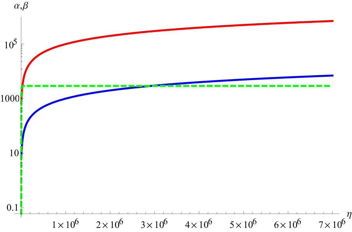 Figure 1
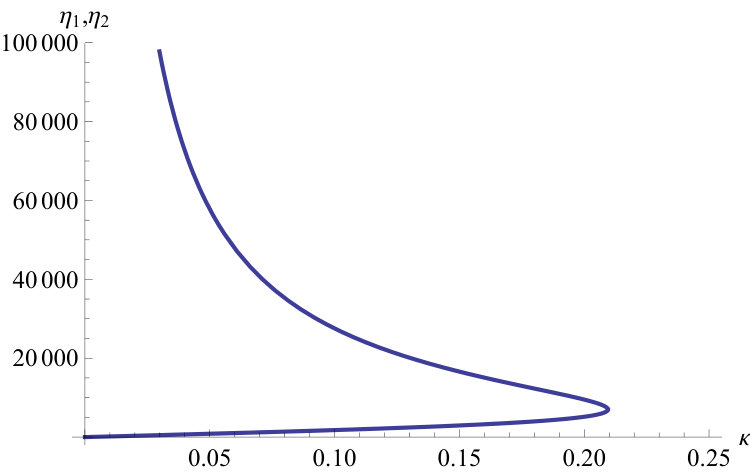 Figure 2
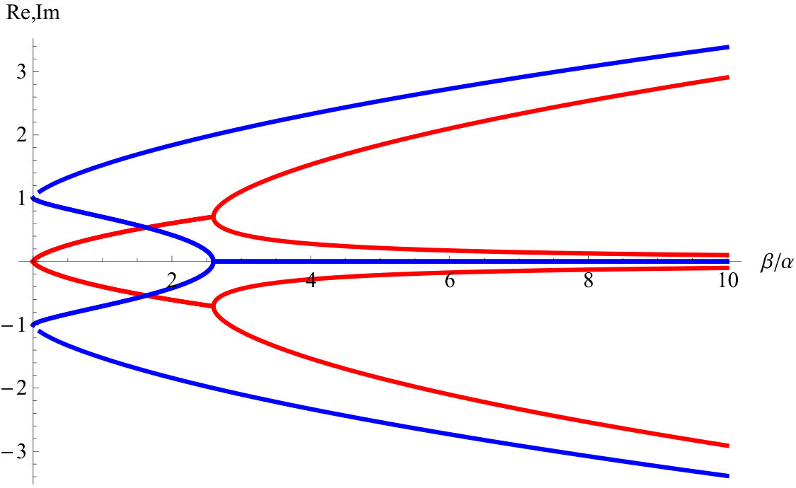 Figure 3
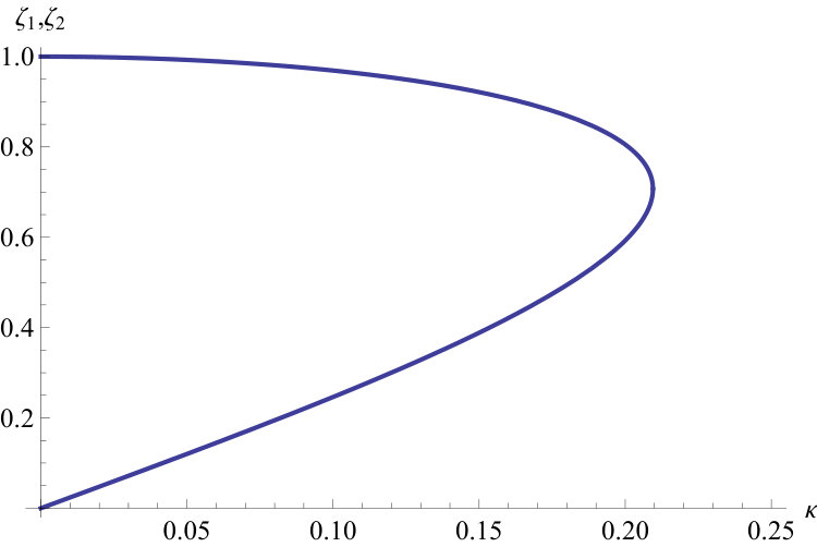 Figure 4
Peer Reviews
No public reviews on file for this paper yet. If you reviewed it on a platform where reviews are public (OpenReview, ICLR, NeurIPS, ICML), you can paste yours below so the community can read it here.
Videos
No videos yet. Explain this paper in a talk, walkthrough, or lecture? Add one.
Fourier-Correlation Imaging
Daniel Braun1, Younes Monjid2, Bernard Rougé2 and Yann Kerr2
1 Institute for Theoretial Physics, University Tübingen, 72076 Tübingen, Germany
2 CESBIO, 18 av. Edouard Belin, 31401 Toulouse, France
Abstract
We investigate to what extent correlating the Fourier components at slightly shifted frequencies of the fluctuations of the electric field measured with a one-dimensional antenna array on board of a satellite flying over a plane, allows one to measure the two-dimensional brilliance temperature as function of position in the plane. We find that the achievable spatial resolution resulting from just two antennas is of the order of , with , both in the direction of flight of the satellite and in the direction perpendicular to it, where is the distance between the antennas, the central frequency, the height of the satellite over the plane, and the speed of light. Two antennas separated by a distance of about 100m on a satellite flying with a speed of a few km/s at a height of the order of 1000km and a central frequency of order GHz allow therefore the imaging of the brilliance temperature on the surface of Earth with a resolution of the order of one km. For a single point source, the relative radiometric resolution is of order , but for a uniform temperature field in a half plane left or right of the satellite track it is only of order , indicating that two antennas do not suffice for a precise reconstruction of the temperature field. Several ideas are discussed how the radiometric resolution could be enhanced. In particular, having antennas all separated by at least a distance of the order of the wave-length, allows one to increase the signal-to-noise ratio by a factor of order , but requires to average over temperature profiles obtained from as many pairs of antennas.
I Introduction
Spatial aperture synthesis is a standard technique in radio-astronomy Interferometry_Synthesis_Radio_Astronomy . It allows one to achieve the fine resolution of a large antenna by correlating time-delayed signals received from the different antennas in an antenna array. In satellite-based remote sensing, spatial aperture synthesis is a technique of choice when relatively long wave-lengths are imposed by the applications, such as the measurement of sea surface salinity or surface soil moisture. When operating in the protected L-band (1400-1427 MHz), a resolution of 10km would require already a single antenna with a size of 32 meters. Spatial aperture synthesis for passive microwave-sensing was therefore proposed to ESA Kerr2001 , and implemented for the first time in the SMOS mission in 2009 that still operates today Kerr2001b ; Kerr2010 . The satellite uses a deployable Y-shaped antenna array and provides a spatial resolution between 27-60km.
With the application-driven need for higher spatial resolution down to the order of 1km, even spatial aperture synthesis leads to forbiddingly large antenna arrays, and there is therefore an ongoing quest for finding alternative concepts (see e.g. camps_two-dimensional_2001 and references therein). Compared to stationary antenna arrays on Earth used for astronomy, one may wonder whether the motion of the satellite could be used for creating a two-dimensional (2D) artificial antenna array out of a one-dimensional (1D) moving array, oriented perpendicular to the motion of the satellite. It turns out that this is not possible when directly correlating the observed microwave fields in the time-domain: the useful phase-shift gained due to the motion of the satellite is, to first order in cancelled by the Doppler shift, where is the speed of the satellite and the speed of light braun_generalization_2016 .
In this paper, we examine another idea: instead of correlating the signals in the time domain, we consider the correlations between their Fourier components at slightly different frequencies. This may appear surprising at first, as, at the level of the sources, the standard model assumption is that different frequencies are entirely decorrelated. Nevertheless, a hypothetical monochromatic point source is seen by different antennas at slightly different frequencies due to the slightly different Doppler effect, and hence it makes sense to correlate different frequency components from different antennas with each other. The useful frequency differences are tiny, down to below one Hertz, and correspondingly long acquisition times are needed. However, one may hope that this opens at least in principal a new way of achieving a resolution of the order of a kilo-meter in passive microwave remote sensing in the L-band by using the motion of the satellite for reducing a 2D antenna-array to a 1D array.
We derive the principles of this “Fourier-correlation imaging” (FouCoIm) technique in detail, and calculate the achievable spatial and radiometric resolution. An emphasis is put on pushing analytical calculations as far as possible, and testing the method at the hand of simple situations, namely a single point source and a uniform temperature field. Estimation of numerical values will be done with a standard set of parameters: km, km/s, GHz, K, MHz, and m. This leads to the important dimensionless parameters , , and .
II Model
We assume that the fluctuating micro-wave fields measured at the position of the satellite are created by fluctuating microscopic electrical currents at the surface of Earth that are in local thermal equilibrium at absolute temperature , where are coordinates of a point on the surface of Earth. The entire analysis will be in terms of classical electro-dynamics. In braun_generalization_2016 we derived the expression
[TABLE]
for the time dependent electric field arising from the current fluctuations at the position of the satellite, with , where is the position of the antenna at time , the speed of the satellite in the Earth-fixed reference frame, the magnetic permeability of vacuum, and the current density as function of space and time. All expressions are in the Earth-fixed reference frame, which is more convenient for the present study than the satellite-fixed reference frame. It was shown in braun_generalization_2016 that (1) is the correct far-field up to relativistic corrections of the prefactor of order (due to the mixing of electric and magnetic fields in a moving reference frame), and the neglect of terms of order in the phase. Eq.(1) does contain in the phase the linear Doppler shift and relativistic effects (including time dilation) up to order . The far-field approximation is justified for , where (of order cm in the micro-wave regime) is the wave-length of the radiation (see Chapt.9 in Jackson99 ).
We substitute the Fourier-decomposition of the current density,
[TABLE]
into (1). The question whether one should differentiate with respect to was answered to the negative in braun_generalization_2016 , but it is irrelevant if we neglect changes of order to the prefactor. We then find the time dependent field seen by the flying antenna,
[TABLE]
with . The Fourier transform of that signal is
[TABLE]
We assume that the current sources can be described by a Gaussian process, where sources at different positions or different frequencies, or with different polarizations are uncorrelated,
[TABLE]
where we have introduced for dimensional grounds a correlation length and a correlation time , and the polarizations are indexed by , taking values . In principle the average is over an ensemble of realizations of the stochastic process, but we may assume ergodicity of the fluctuations, such that they can also be obtained from a sufficiently long temporal average. In practice this means that one should average over positions considered as equivalent in terms of the ensemble, i.e. the time the satellite takes to fly over a desired pixel size. For a satellite flying at a speed of order km/s and a pixel size of order km, this means a maximal averaging time of the order of a second. This does not preclude calculating Fourier transforms with finer spectral resolution from data acquired over much longer times.
We will make the assumption that only the current intensities at the surface of Earth contribute. In reality the emission seen by the satellite arises from a thin surface layer on Earth that has a finite thickness of the order of a few centimeters Kerr2010 ; Kerr2012 , depending on the soil and its humidity, and the satellite also sees the cosmic microwave background. We approximate the surface layer as a single plane located at , i.e. and neglect the cosmic microwave background as its temperature is two orders of magnitude lower than that of Earth, as well as other astronomical objects.
The current intensities are related to an effective temperature by
[TABLE]
where is a constant (see eq.(105)). Eq.(7) is valid for and hence very well adapted to micro-wave emission at room temperature.
Eq.(6) together with (7) is a standard model of classical white noise currents, and appears in many places in the literature, see e.g. eq.(4.16) in sharkov_passive_2003 . The equation is an instance of the fluctuation-dissipation theorem that can be found in standard text-books on statistical physics (see e.g. Part 1, Chap. XII and Part 2, Chap.VIII. inLLStatMech80 ). In the context of thermal radiation it goes back at least to the original Russian version of rytov_theory_1959 (from 1953); see also Rytov89 . The model has also been used to study coherence effects in the thermal radiation of near-fields (see eq.(3) in carminati_near-field_1999 ). For completeness, we present the derivation of (7) in the appendix, based on Planck’s law for the energy density of an e.m. field in thermal equilibrium.
Compared to a black body, the emissivity of a real body is modified by a mode-dependent emissivity factor , where is the direction of emission (from the patch on ground to the satellite), and a factor of geometrical origin that takes into account the variation of the radiation with respect to the surface normal (i.e. the projection of the area of a patch of the surface onto the plane perpendicular to the propagation direction). The temperature is then really an effective temperature, , where the brightness temperature is defined as the absolute temperature a black-body would need to have in order to produce the same intensity of radiation at the frequency and in the direction considered (see Appendix X.1.1). For simplifying notations, in the following we keep writing for short instead of , but keep in mind its physical meaning, which, after all, is crucial for data-analysis and fitting vegetation and surface models to observational data Kerr2012 . We thus arrive at the current correlator
[TABLE]
which can be considered the statistical model underlying the imaging concept, and .
III Correlation of Fourier components
For each antenna, the electric field component is transduced into a voltage . We denote the frequency response of the antennas and eventual subsequent filters by the complex function , the Fourier transform of the time-dependent response function of antenna and filter. In the frequency domain we have simply . With (8) we obtain the correlation function between the voltages at two different frequency components , measured at the positions of the antennas with original positions and ,
[TABLE]
where now , and . The correlation function is the filtered version of the original unfiltered correlations . We see from (9) that the latter can be obtained from the former simply by dividing through the product of the known filter functions, as long as the latter are non-zero. Of course, outside the frequency response of the antennas and filters, the measured correlations vanish due to the vanishing of and do not carry any information anymore. This will ultimately limit the frequency range over which information on the brightness temperature can be extracted, or, equivalently, leads to a finite geometrical resolution even if a known for all frequencies would lead to perfect resolution. However, this appears only when inverting the measured signals and will be discussed in section V.1. For the moment we assume that we have access to the unfiltered through (9) for all frequencies that we need, and base the general development of the theory on .
We change integration variables from to “center-of-mass” and relative times, and , and introduce as well a new integration variable for the spatial integration, . This implies and . The Jacobian of both transformations is equal to
- Furthermore, from now on we take the satellite to move in direction, , where is the unit vector in direction. This leads to .
The total phase appearing as arguments of the exponential functions under the integrals in (11) is
[TABLE]
We see that only appears as prefactor of in the phase (12), and as argument in . The integral over therefore boils down to a 1D Fourier transform of the intensity of the current fluctuations in the direction of the speed of the satellite, with conjugate variable proportional to the difference of the frequencies of the Fourier components that we correlate. This can be made more explicit by introducing a position variable along the path of the satellite. For the conjugate variable we define . We write and not in order to distinguish this “wavevector” from the usual one obtained from a single frequency and dividing by . We also introduce the “center of mass frequency” . It will be called “center frequency” in the following for short, but should not be confused with the central frequency that is the fixed frequency in the middle of the band in which the satellite operates (e.g. 1.4 GHz for SMOS). With all this, we see that
[TABLE]
We have defined , where is understood, and the spatial Fourier transform of the temperature field in -direction. This notation makes clear that in these coordinates the temperature depends both on and , even though the motion of the satellite combines the two arguments in a single one, . We can think of as the Fourier image of with respect to the coordinate, calculated with a starting point . I.e. for all , we have a 1D spatial Fourier transform of the intensity of the current fluctuations where the Fourier integral is defined with origin in . The Fourier images obtained by translation of in -direction are not independent. Rather we have
[TABLE]
We are thus led to
[TABLE]
We neglect the slow dependence of compared to the rapid oscillations of the phase factors in (III) and pull it out of the integral as a prefactor . We can then perform the integral over , and find
[TABLE]
We introduce center-of-mass and relative coordinates for and , and . We further restrict to values much smaller than . This implies a limitation of the integration range for when calculating the Fourier components, but it is a mild one. Since , it is enough to have , which is typically of order s, and therefore gives time to resolve Fourier components down to a hundredth of a Hertz. We can then approximate to first order in ,
[TABLE]
Neglecting terms of order and of order in the prefactor of the exponential, as well as a second order term of order in the phase, the integral over the Dirac -function gives
[TABLE]
and . The unit vector is obtained by taking the original center of mass position of the antennas at , and . Eq.(20) is one of the central results of this paper. It shows that the two-frequency correlation function of the fields at different antenna positions is related linearly via a 2D integral-transformation to the brightness temperature field in the source plane, or more precisely to the Fourier transform of that field in -direction. With defined on a 2D grid, the reconstruction of from the measured correlation function thus becomes a matrix inversion problem that has to be performed numerically in general. A crucial question is the conditioning of the inversion problem. It will be studied in more detail in a subsequent paper dedicated to a numerical approach NumPaper .
Here we give a simplified analytical treatment that allows us to obtain estimates of the spatial and radiometric resolutions, and thus provide evidence that the inversion problem is sufficiently well conditioned for the reconstruction of from the measured . For this, we study the situation where the vector from antenna 1 to antenna 2 is orientated in direction, , in which case , and denotes the spatial separation of the two antennas.
We switch to a dimensionless representation by taking as length scale the distance between the two antennas. We will express all other lengths in this unit, and introduce the dimensionless coordinates by , , and . The dimensionless height is for the standard parameters . Eq.(20) then reads
[TABLE]
where . The 1D integral kernel
[TABLE]
which is itself defined through an integral over . For fixed , , , and , the integral kernel is a function of that relates the 1D Fourier transform to the observed correlation function by integration over . Suppose that the integration over can be inverted by finding the inverse integral kernel. Integrating the inverse kernel over with the correlation function measured as function of the center frequency , we then obtain for all and the chosen . If this can be done for all relevant , we obtain for each point on the axis the Fourier transform in direction of the intensity of the brightness temperature. Taking the inverse Fourier transform in -direction, we obtain the full - and -dependent brightness temperatures. To proceed, we first study the integral kernel in the relevant parameter regimes.
IV Properties of the integral kernel
The arguments of are given by eq.(21) as
[TABLE]
By their definition, we only need . For we can consider that in the end the maximum should be of the order of the inverse resolution required in direction. Taking of the order of one km, and using the standard parameters, we get . With varying from (in reality, the extension of Earth limits the integration range to a maximum value of the order ), reaches its maximal value for . For standard parameters, 1.4 GHz, . Both and can be positive or negative, such that there is also a regime, where , and we will find that this is the most important one. Note that from (22) we immediately obtain the relations
[TABLE]
We therefore restrict the following discussion to .
Unfortunately, the integral over in (22) cannot be done analytically. However, we can find approximations for different cases. Consider first . Using the methods of residues, one easily finds
[TABLE]
More generally, one can obtain a useful expansion for small by expanding into a power series, and then integrating term by term. We find
[TABLE]
where is the modified Bessel function of the second kind of order . The zeroth order result (26) is recovered by observing that . For small the series converges rapidly, and one can even improve the agreement with the numerically calculated kernel by re-exponentiating the first few terms. For example, up to second order we have a polynomial which we wish to write as . Expanding the exponential in powers of and comparing powers up to order , one finds and . When plotted together with the exact result, the thus obtained approximation agrees with for visibly well up to , i.e. well beyond the regime . For the fourth order re-exponentiated form the agreement extends up to about . However, the exponential decay (26) already of the zeroth order term with indicates that for the values of to the contribution to the integral for values such that is of order of or smaller than one, can be entirely neglected.
In the opposite regime of large , an approximation based on a stationary phase approximation can be found. More precisely, one needs . In that case one can treat as a slowly varying factor compared to the rapidly oscillating . The point of stationary phase of the latter term is found at (where the function has a maximum). The second derivative of the phase at equals 1. With this we get
[TABLE]
valid for . Interestingly, the integral kernel becomes independent of in this regime, which is of course a consequence of the fact that the stationary phase point is at , thus eliminating the factor in the phase of the prefactor. We furthermore see that in this regime there is no exponential suppression of the kernel.
For , the kernel can be evaluated exactly,
[TABLE]
where is the zeroth Bessel function, and the zeroth Struve function. Their asymptotic behavior gives back (29).
In Fig.1 we plot as function of . We see that a regime exists for , which defines (see after eq.(32) for its precise value). For , . The regime is also possible, but it is restricted to a tiny interval, such that its contribution to the integral over is negligible. For , the stationary phase points of become relevant. Fig.1 shows the Im- and Re-parts of the six roots of the corresponding stationary phase equation. We see that only for real stationary phase points exist. Since on the other hand occurs for sufficiently large for almost all only for (see Fig.1), the kernel is exponentially small in this regime . Altogether, the only relevant regime is thus .
While the asymptotic form of the integral kernel suggests the use of the orthogonality relations of Bessel functions, inverting (20) is nevertheless non-trivial due to the more complicated dependence of and on . However, the above asymptotic form allows one to obtain an approximate analytical inversion of the kernel that allows for an estimation of the resulting resolution, as we will show now.
V Estimation of geometrical resolution
V.1 Approximate analytical inversion of the integral kernel
At first sight, the requirement appears unnatural given that can already of the order to . And indeed, this leads to a first rather stringent condition which must be met in order for the correlation function to be non-zero. In terms of the original parameters, . For this to be much larger than one, one needs
[TABLE]
or , where we have used already the maximum value of the function of on the left hand side (lhs) in (31). For the standard parameters, we find . When operating at in the GHz regime, this means that the correlation function essentially vanishes for larger than a few Hertz and thus bears no more information for the measurement of the position dependent brightness temperature.
Another way of seeing this is to observe that (31) limits the integration range for : The lhs of (31) is a function that starts of at [math] for , increases linearly, reaches a maximum of at , and decays as for large . Condition (31) then limits the integration range of to an interval with
[TABLE]
where , , and (see introduction and Fig.2). A finite real integration range exists only for , equivalent to . For given , we have . A finite minimal value of can be deduced from a maximum desired snapshot size in direction. Also the requirement may bound the relevant values of from below, as it leads to a smallest resolvable frequency, and thus also smallest resolvable : .
As the contributions from areas outside the allowed range (or, correspondingly for negative , ) are exponentially suppressed, we can limit the integration range of to that interval for a given , and replace the integral kernel by its approximate form, eq.(29), extended to by (25), yielding
[TABLE]
in the allowed range, and zero elsewhere. After the substitution , the result for can be written as
[TABLE]
where (with , ), and is a window function equal to one for and zero elsewhere. The window functions translate in a straight forward fashion the integration range for into an integration range for . By definition, ranges from . So , lie within this interval, , and the window functions take care of restricting the argument of the integrand to the intervals . We have replaced by the equivalent information (related to ) and (related to ), and consider only. Given eq.(34) it is tempting to try to recover by Fourier transform. However, the functions that appear in prevent (34) from being a simple Fourier integral. Moreover, from the measured data we only have , the filtered version of , that is restricted to a frequency range , where is the bandwidth (20MHz in SMOS for the L-band). We assume here for simplicity a Gaussian filter and the same for both antennas. For a real filter response function , its Fourier transform must satisfy . Taking also as real, we can write it as
[TABLE]
where is a normalized Gaussian centered at with standard deviation . The factor assures that for , is normalized according to . Under the same condition we have
[TABLE]
where , and . This contains the approximation of using only the “diagonal” terms in the product of , i.e. the ones with , which is justified by the fact that . Fourier transforming with respect to (denoted by ) gives a convolution product between the FT of the Gaussians (which is ) and , and leads to
[TABLE]
where we used that the sign of in (37) determines the one of in (35). Thus, we get back the original function , cut by the two window functions and multiplied with , convoluted with the product of a Gaussian of width and a rapidly oscillating cosine function. The factor can be tracked back to the change of variables from to and will distort the image at the nadir and at infinity. Sources at positive or negative contribute differently due to the different sign of the phase shift. This arises already in (33) due to the different phase shift in the asymptotics of the Struve functions for negative or positive arguments and leads to the sum over . In general, an exact inversion can not be simply done by Fourier transform but needs a numerical approach. Nevertheless, we can arrive at an estimation of the resolution by considering a single point source, as then only one of the two terms in the sum over in (V.1) contributes, and the factor becomes a simple numerical factor given by the position of the source.
V.2 Single point source and geometric resolution
V.2.1 Correlation function and reconstructed image
Let the point source be at position and with polarization , where is situated in the allowed range for some in the desired range up to the largest considered , where is the pixel size. We thus have
[TABLE]
which together with eq.(16) yields
[TABLE]
As is in the allowed range, we can use the approximate analytical form of the integral kernel, eq.(33), to get from eq.(34) the correlation function
[TABLE]
where is the Heaviside theta-function. Considering (V.1), we may define an approximative reconstructed source function suitable for sources at through
[TABLE]
where is a normalization constant. Due to the dependence of the window functions, and the dependence of the integral transform as compared to a simple Fourier-transform of , one cannot get a normalization constant independent of the source field. In particular, for the single point source, would depend on the position of the point source. However, we use only for estimating the geometric and radiometric resolution. For the former, all prefactors are irrelevant. For the latter, we avoid the problem by calculating relative uncertainties of only, where any prefactor cancels. We hence set in the following.
Inverting the Fourier transform in leads to
[TABLE]
This equation is valid for all sources located in the positive plane, not necessarily point sources. When we re-express the correlation function through (34) and perform the Gaussian integral over , we find a direct approximate formal relation between the FT of the original in the upper half plane, and its reconstructed image ,
[TABLE]
Using this expression, or by inserting (42) into (37), and the resulting filtered correlation function into (44), we find the reconstructed image of the single point source
[TABLE]
where , , and .
V.2.2 Geometric resolution
We see that the reconstructed image of the point source is a series of narrow peaks spaced by the inverse of due to the rapidly oscillating -function, under an approximate Gaussian in -direction centered at the position of the source with a width in given by . It reminds one of a diffraction image from a double slit, even though there the envelope is a -function, not a Gaussian. Nevertheless, we adapt the definition of resolution from that example, namely that the best resolution is obtained from the smallest shift that makes a peak move into the next trough. This leads to
[TABLE]
hence . For , this is of the order . The numerical value for the standard parameters gives 2.1 km, i.e. a resolution of the order of a kilo-meter. However, for actually achieving this resolution for an extended source, one has to face two issues: i.) The reconstructed point-source image should be brought as close as possible to a single narrow peak; and ii.) one has to deal with the different phases from sources at positive or negative . The first issue can be addressed by superposing correlation functions from pairs of antennas at different separation, and/or changing the considered central frequency. This shifts the pattern of peaks due to the cos-function, and one can engineer a rather narrow central peak (see NumPaper for details). The second issue should be absent in a numerically exact inversion of the integral kernel. The Gaussian envelope has a width given by the inverse bandwidth, which is much larger than the width of a single peak, namely by a factor for the standard parameters.
The resolution in -direction follows from the effective wave vector in the function. It depends on the position of the source and reaches its maximum possible value for (i.e. ). The inverse of thus gives the best possible resolution in -direction:
[TABLE]
We conclude that both in - and -direction one can expect a geometric resolution of the order for sources close to . For sources close to , goes to zero , whereas for larger the decay of is . The geometric resolution in -direction deteriorates correspondingly. The resolution in -direction, on the other hand, depends only weakly on the source-position, as increases monotonically from at to at , and keeps growing slowly beyond . It is remarkable that correlating electric fields at two different frequencies can lead to a resolution that is given by the central frequency.
The definition of is based on the request that the stationary phase approximation (SPA) holds in the regime . In practice, the SPA is almost always better than expected, such that in the end the result might be a conservative estimate of the geometric resolution.
VI Radiometric resolution
Besides the geometric resolution, the radiometric resolution (RR), i.e. the smallest difference in temperature that the system can measure for a given pixel, is the most important characteristics of the satellite imaging system. Here we calculate the RR for the idealized situations of a single point source considered above and for a uniform temperature field in the positive half-plane .
VI.1 Fluctuations of the reconstructed temperature profiles
The idea behind the calculation of RR is that the electric field measurements yield random values, whose fluctuations and correlations reflect the thermal nature of the radiation field. Thus, if with the same field one repeated the measurements many times, one would obtain different correlation functions in each run, and thus, after inverting the linear relationship between and , also different reconstructed (called in the following) in each run. The (relative) RR is then defined as the standard deviation divided by the average for a given position . In general it will vary as function of , and also depend on the temperatures at all positions, a behavior well known from standard spatial aperture synthesis. In reality, things become still a bit more complicated, as the measured signal is a superposition of the e.m. field emitted by the antenna itself (at temperature ), and the radiated field from the surface of Earth. However, these fields are uncorrelated, and their averaged squares just add up. For simplicity, we will neglect the noise contribution of the antennas in this first analysis, which amounts to calculating lower bounds of .
Starting point of the calculation is the assumption that the current fluctuations which are at the origin of the radiated thermal field are described by a random Gaussian process, both in time and space (see sec. II). This implies immediately, that also the temporal FT of the current fluctuations is a Gaussian process, now over space and frequency. Finally, the connection between and is linear, which implies that is a Gaussian process over and . By the nature of this variable, it is a complex Gaussian process. One easily shows that the average of equals zero (if the average of all current components is, which must be true at thermal equilibrium). The correlation function is the (complex) covariance matrix of this Gaussian process, and all higher correlations can be expressed in terms of it.
In order to assess the fluctuations of we first define a product of Fourier coefficients of from a single run (denoted by a ),
[TABLE]
and its corresponding filtered version (with expressed in terms of ).
The fluctuations of are defined as , where the average is over the thermal ensemble. With from (44), one finds
[TABLE]
It can be shown (see Sec.X.1.2) that in the narrow frequency intervals considered here the Gaussian random processes given by the is circularly symmetric. It hence enjoys the property (see eq. 8.250 in Barrett03 ),
[TABLE]
where we have abbreviated . The correlation function contained in the large parentheses of the second line of (51) becomes
[TABLE]
with , , and where we have used .
The fact that and in (53) contain the same position arguments twice makes that we cannot evaluate it directly through eq.(21), as the coordinate transformation to dimensionless variables based on the rescaling with becomes singular. We therefore have to go back a step to eq.(20) which yields
[TABLE]
Comparing with (21) we see that this result corresponds formally to in that equation, rather than , and (55) is recovered by using the exact result (26). We can now re-introduce dimensionless variables via the same rescaling with , where, however, is still given by , and denote as before the positions of the two antennae at , only one of which still enters as argument in , respectively . This gives
[TABLE]
We calculate for the single point source considered in Sec. V.2 at the position of the source, i.e. , and for a uniform temperature field.
VI.2 Single point source
For the single point source at position , the correlation function becomes (see (41))
[TABLE]
Insert this into eq.(51) to find
[TABLE]
We change integration variables to . The Jacobian is 1. In the product of the Gaussians only the diagonal terms (i.e. with the same signs in front of ) contribute in the relevant regime , as for opposite signs . Finally, we approximate
[TABLE]
and pull that factor out from the integral which is permissible for all ranges of variables for which the product of Gaussians is non-negligible. The integrals can then be performed, and we find for the standard deviation
[TABLE]
where in the last step we have used that and (where once more ).
From (46) we find
[TABLE]
Combined with (60) we obtain the relative RR
[TABLE]
For , the relative RR is of order 0.055, corresponding at K to K.
VI.3 Uniform temperature field
We now look at the second standard situation considered commonly for the determination of the radiometric resolution, namely a field of constant temperature. More precisely, we consider
[TABLE]
The restriction to sources in the upper plane is due to the fact that we still want to use eq. (44) for calculating the reconstructed temperature profile. The cut-off arises physically from the size of the Earth and prevents a divergence of the correlation function.
From (13) we obtain
[TABLE]
The correlation function (56) becomes
[TABLE]
with . For km the radius of Earth, and m, . We see that here the correlation function is perfectly diagonal in frequency, which of course reflects the lack of structure of the temperature field in -direction. Hence, we can set everywhere , which greatly simplifies the analysis. The cutoff in eq.(65) prevents a logarithmic divergence that arises from for . Eq.(65) can be extended to a temperature field that is uniform everywhere from to . In this case, the -integral starts at rather than at 0. However, in this situation we cannot use (44) anymore as it is valid only for sources at positive (see the discussion after (V.1)).
Eq.(65), when inserted into (51), and with the same change of integration variables and approximation (59), leads to
[TABLE]
The reconstructed temperature field (45) is given by
[TABLE]
Unfortunately, no closed analytical form could be found for the remaining integral, and even a numerical evaluation is not straight forward, as the Gaussian yields a very narrow peak, broader, however, than the period of the -function. But we can get an estimate of by replacing the Gaussian (normalized to an integral equal 1) with a rectangular peak of width and height centered, as the Gaussian, at . Here, , and is a parameter of order 1. This gives
[TABLE]
A numerical evaluation of the integral is now relatively straight forward and shows a slowly varying as function of in the interval , whereas outside this interval it oscillates rapidly. The slow variation arises from the factor that distorts this approximately reconstructed image. Pulling out this slowly varying factor in order to get an analytical estimate of the order of magnitude of , we are led to
[TABLE]
for . Hence, in this interval and apart from the distorting factor identified previously, we recover a constant temperature field. The value of the reconstructed temperature depends on the precise value of as well as the ratio . Outside the mentioned interval, oscillates again as function of , which can be understood from the fact that the box is cut-off when gets within a distance of [math] or . The sought-for order of magnitude can be estimated from the maximum value of (70) as function of . As for standard parameters , we can bound the -function by one (while still having ), in which case we obtain in the mentioned -interval. With all this, and approximating in the logarithm in (67), we find the order of magnitude For , this is of order for standard parameters, i.e. a catastrophically large uncertainty. A small value of is possible only if is very small, but apart from the fact that one should not rely on this image-distorting factor, it could only be sufficiently small for unrealistically close to the nadir.
If one traces back the difference to the single-point source, one realizes that while scales in both cases as , the difference comes from itself: for the single point source it is of order , but for uniform in the upper half plane of order , which explains a factor worse relative RR for the latter compared to the former. The factor in the single-point arises from the cut-off of the integral: scales as , and for the -integral in (44) just gives a factor , as the correlation-function is independent of in this case. On the other hand, for constant temperature in the upper half-plane, the cut-offs do not play a role, as the -function picks up only . This leads to the loss of one factor in . The second one comes from the integration over in (68): the rapidly oscillating -function leads to a factor , whereas for the point-source only a single point contributes, such that the cosine is of order one.
In the light of the RR of standard radiometers that typically scales as , where is the integration time, the fact that in eqs.(60,67) is independent of the bandwidth is rather surprising. Formally, the disappearing of can be traced back to using the lowest order in the Laplace approximation of (58). The next order corrections are of order , such that . One expects the sign of the correction to be positive, as the integrand is positive everywhere, and the lowest order approximations amounts to replacing the Gaussians by normalized Dirac-delta functions. Hence, for small but finite , is expected to increase with , which is contrary to the behavior of standard radiometers. Standard radiometers are based on the van Cittert-Zernike theorem, which gives the reconstructed temperature field as Fourier transform of the observed visibilities at a fixed frequency. Different frequencies at the source are uncorrelated, and the scaling of just reflects averaging over a number of independent measurements that scales . In FouCoIm the information is in the correlation between different, very narrowly spaced Fourier components, and averaging over the central frequency does not lead to additional information (see also Sec.VII.2). Therefore a larger bandwidth does not improve RR.
VII Noise reduction
The bad signal-to-noise ratio for the radiometric resolution in the case of a uniform temperature field in the upper half plane, makes it essential to consider measures that lead to a noise reduction and in particular averaging schemes.
VII.1 Averaging over time
Instead of examining , we consider here for simplicity directly the fluctuations of the measured ”single shot” correlation function . The first idea that comes to mind for reducing the fluctuations of is to average over the origin of the time-interval from which we construct the Fourier transform. Note that this is very different from an ensemble that one would obtain by displacing the initial position . But averaging over the origin of time only leads to an overall factor:
[TABLE]
So it is obvious that this kind of averaging is useless. This is indeed to be expected, as all available data were already used. The situation improves only slightly if the FTs are calculated from a finite stretch of data (say over a duration ). Then shifting the origin in time will include some new random data, but since we must have , it is clear that we still use essentially the same data with the exception of some new data points at the edge of the interval of length .
VII.2 Additional frequency pairs
Using only a small frequency separation of width about the central frequency which itself is allowed to vary over a large bandwidth appears to be a very wasteful use of all the pairs of frequency components . Can we use different measured correlations with sufficiently different as independent data for improving the radiometric sensitivity? In order to answer this question, we need to calculate the covariance matrix between two different correlators,
[TABLE]
as well as the pseudo-covariance matrix ,
[TABLE]
Both matrices together determine the statistical properties of the random process . Note that despite the fact that can be considered a circularly symmetric Gaussian process (see Appendix) over and in the narrow frequency band we are interested in, the same is not true for (which is not even Gaussian). We need to know whether both and essentially vanish for almost all pairs of pairs of frequencies, with the first pair in a first region (notably in the central narrow strip ), and the second pair in another region in the plane that we may want to consider, whereas the correlation functions and themselves should still be non-zero. Such a situation would signal statistically independent non-vanishing correlation functions. However, we saw that only within a central narrow strip (whose width is given by ) in the plane is non-zero, and within that strip all pairs of frequencies are used for obtaining a single profile . Here we show the same thing once more by proving that for and to vanish the second pair of frequencies must be not in — where, however, vanishes.
To see this, one first shows with the help of (52) and in a few lines of calculation that
[TABLE]
We have from (56), where now , and correspondingly for . Whether are large or small can be judged by comparing it to the product of the standard deviations of each factor. This corresponds to calculating Pearson’s product-moment coefficients pearson_note_1895 and where we define, for complex , , and , for short. Going through the same calculation as for , we find after some algebra
[TABLE]
where
[TABLE]
and hence . This implies
[TABLE]
For we have
[TABLE]
where
[TABLE]
with , , , and . From the properties of the integration kernel we know that vanishes iff , and correspondingly for . Hence, for and and all of order , we need or . Note that .
For determining the properties of , we consider our two previous cases of sources.
Case 1: Single point source. Here we have independent of , see eq.(41), which inserted into (79) yields
[TABLE]
and hence
[TABLE]
For sources at , we have therefore iff or where Hz.
Case 2: Constant temperature field in the positive upper half plane. Here, is given by eq.(64). Hence, as soon as or . Of course, the function in (64) arises from the complete lack of structure of the temperature profile in -direction. More realistic is at least a cut-off at the size of Earth, which we take as the same as in direction. In that case one finds and hence
[TABLE]
The exponential factor in the integral makes again that vanishes essentially if for or .
Comparing with the situation for , we find that for both types of sources considered, vanishes much more rapidly as function of the separation of two frequencies, as there is no factor multiplying . Hence, the request for vanishing is more restrictive.
The question of the usefulness of considering other frequency pairs can now be phrased as: Can one find pairs of frequencies such that or while still , for all frequencies with used in the reconstruction of a temperature profile from ? For a single frequency pair all conditions can be easily satisfied. It is enough that both pairs and be inside the strip , and at the same time far away from each other, i.e. , which implies and at the same time. However, the difficulty arises from the fact that we use already all pairs in the full available band-width for the reconstruction of a single temperature profile. This can be seen e.g. from eq.(V.1), where we integrate over all for recovering . Hence, there are really no new frequency pairs that can be used for improving the signal/noise ratio of the reconstructed temperature profile.
The same conclusion can be arrived at more formally by calculating the correlations between temperature profiles obtained from different center frequencies. Let be the reconstructed temperature profile given by eq.(44), where we now keep explicit the dependence on the center frequency , hidden in that equation in the filter functions , see eqs.(37,38), and is understood, so as to get the temperature profile from a single realization of the noise process. We define the correlation function
[TABLE]
and its renormalized dimensionless version
[TABLE]
that obviously satisfies . We have
[TABLE]
where , , , , (), with (see eq.(36)), and we have used that . We evaluate for the case of constant temperature in the upper half plane. Using (73), (65), and switching momentarily to integration variables , and then back to , we are led to
[TABLE]
The integral is clearly real, as it should. The integral over leads, when integrated from to to a divergent factor, but that factor cancels (together with the remaining prefactor ) when we consider the re-scaled version of the correlation function . If we set , it is clear that the only remaining scale for is . The remaining integral over in (90) can in fact be evaluated analytically. The result is too cumbersome to be reported here, but plotting it as function of shows that indeed the correlations decay only on a scale of order . This proves that by shifting the center frequency within the available bandwidth one cannot gain independent estimates of that would allow one to improve substantially the signal-to-noise ratio.
VII.3 Additional antennas
So far we considered only two antennas. As mentioned before, in order to obtain a reconstructed single source image with a single peak, one may sum the correlated signals from several antenna pairs. It is to be expected that this will reduce , but we have to figure out how far two pairs of antenna have to be separated in order to produce essentially uncorrelated correlation functions. To answer this question, we have to generalize eq.(73) to pairs of correlators at different points . We define
[TABLE]
where we take for , i.e. the antennas in the second pair are shifted by distance in -direction compared to the corresponding ones in the first pair. From (52) we have
[TABLE]
[TABLE]
The corresponding result for is obtained from the last line in (93) by replacing . For the uniform temperature field in the upper half plane up to a cut-off and also a cut-off of the same value in -direction, we have for . No closed form was found for the remaining integral over , but a closed form is easily obtained if we neglect the slowly varying envelope , which is legitimate for cut-offs not too close to 1 and gives an idea on which length-scale will vanish. Plotting the results of the integration one finds that both real and imaginary part decay on a scale of , where we have used again . Hence, for the correlation functions of two pairs of antenna to decorrelate, it is enough that one antenna in one pair be at a distance of order , i.e. of the order of the central wave-length with respect to at least one antenna of the other pair. For standard parameters, this is of the order 10 cm, neglecting factors of order 1 (the helps of course, but for the imaginary part of there is a comparable factor in the scale). Extending the separation of the two antennas in the original pair to m, one would have place for about 2000 antennas in between. This in turn would then allow to be built correlations from pairs of antenna, where the antennas in each pair are still separated at least by m. Considering that averaging of temperature profiles obtained from statistically independent correlation functions improves the signal-to-noise ratio of the average temperature profile by a factor , we can improve the SNR by a factor . If considering the prefactors of order one, 10 times more antennas can be used, the SNR could be improved by a factor . But even such a large improvement is not yet sufficient to beat the low SNR of order . It is quite likely, however, that a displacement of an antenna also in direction by a distance of the order leads to a completely decorrelated correlation function. If so, one might gain another factor up to in the SNR by considering quasi-1D antenna arrangements, with a width in -direction of order 10 meters. In the latter case one should then be able (after averaging temperature profiles obtained from some correlation functions from that many pairs of antennas) to achieve an SNR of , and hence a RR of order of a few Kelvin. However, it is obvious that the effort for doing so is humungous, and the same geometrical and radiometric resolution might be achievable more easily with other means.
Other interesting ideas of improving the SNR involve using focussing antennas for increasing the flux, and/or exploiting higher order correlation functions as well, but these are beyond the scope of the present investigation.
VIII Discussion
We examined the fundamental feasibility of a new type of passive remote microwave-imaging of a 2D scenery with a satellite having only a 1D antenna array, arranged perpendicular to the direction of flight of the satellite. We analyzed the simplest possible configuration of only two antennas. The scheme is based on correlating Fourier components of the observed electric field fluctuations at the position of the two antennas at slightly different frequencies and , and leads effectively to a mapping of the 2D brightness temperature as function of position to correlations as function of the center frequency and the frequency difference . With two antennas separated by , center frequency and a satellite flying at height , the resolution both in - and -direction is of the order . Only very small frequency-differences lead to correlations of finite, useful magnitude. For typical intended SMOS-NEXT values they are of the order of at most 10Hz, which, however, still have to be divided by the number of points in direction that one wants to resolve within a snapshot. This implies that one must be able to measure GHz frequencies with accuracy of the order of a 1/10-1/100 Hz. The speed of the satellite only enters in the maximum frequency difference useful for correlating the signals, which is given by .
In the minimal situation of two antennas, the relative radiometric resolution is, for a single point source of order , whereas for a uniform temperature field in the positive half plane (up to some large cut-off of the size of Earth), which for standard parameters is of order . We have neglected so far the additional noise that comes from the antennas themselves, such that our results should be considered as lower bounds for . Unfortunately, this large uncertainty prevents a direct application of the method with just two antennas, and massive noise reduction is required. Some ideas are discussed in Sec.VII, where it was found that one can obtain statistically independent correlation functions by displacing one antenna by a distance of the order of , where is the central wave-length. Hence, the signal-to-noise ratio can be massively increased by a factor when using the correlations from pairs of antennas from antennas separated all by at least a distance of order . However, the computational effort and the size of the overall structure appear forbiddingly large for achieving a radiometric resolution of order of a few Kelvin with a geometrical resolution of order one kilometer.
An alternative application might be the precise localization of very strong point sources that by far dominate the more or less uniform background from Earth’s thermal emission. As long as one is not interested in a very precise measurement of the intensity of the source, one might localize it very precisely using just two widely separated antennas. These need not even by an board of the same satellite. By having two satellites with well-known distance separated by about 100km for instance, the geometrical resolution achievable in the microwave regime would be of the order of a meter in both and direction and with rather small computational effort, opening interesting perspectives for such applications. It should also be kept in mind that the method can be easily transferred to other types of waves, sources, and media. For example 2D ultra-sound imaging might be possible by beating the signals of just two moving microphons. Different physical systems can be easily mapped to each other by comparing the corresponding dimensionless parameters introduced in Sec.I.
IX Acknowledgments
The authors are very thankful to the CESBIO SMOS team and the CNES project management, without whom this work would not have succeeded. We have more particularly appreciated the technical support from François Cabot, Eric Anterrieu, Ali Khazaal, Guy Lesthiévant, and Linda Tomasini.
X Appendix
X.1 Current fluctuations and temperature
The connection between the intensity of the current fluctuations and the local temperature can be found e.g. in sharkov_passive_2003 ; rytov_theory_1959 ; Rytov89 ; carminati_near-field_1999 . For being self-contained and relating to the notations used in this paper, we here give a short derivation of this connection. We also show that is, in the frequency range considered, a circularly symmetric Gaussian process.
X.1.1 Thermal radiation
We begin by recalling the energy density of electromagnetic black body radiation at frequency , , where is the density of states (number of modes between frequencies and per volume), and the thermal Bose occupation factor, with the Boltzmann constant, and the absolute temperature of the radiation field. An infinitesimal patch on the surface at position with surface and temperature in thermal equilibrium with the radiation field in its immediate vicinity, radiates off an amount of energy per unit time and at frequency given by in direction with respect to the the surface normal. The energy density for both polarization directions received at the position of the satellite at distance from this patch also varies , and energy conservation requires
[TABLE]
Earth is rather a grey than a black body, and we therefore have to include the emissivitiy of the patch in the direction of the satellite given by polar and azimuthal angles. It can also depend on polarization, which we skip here for simplicity. Integration over the whole radiating surface gives the entire energy density at the position of the satellite at this frequency,
[TABLE]
In the microwave regime and temperatures , is about four orders of magnitude smaller than , such that the Bose factor becomes, to first order in , , with corrections of order . This simplifies to
[TABLE]
where we defined the brightness temperature , i.e. the absolute temperature a black body would need to have for producing the same thermal radiation intensity at the frequency and in the direction considered, specified explicitly by the two angles . At the same time, the total energy density (integrated over all frequencies) at position of antenna 1 is , where the average is over the thermal ensemble, but due to ergodicity we may also average over time, . In the end one should take the limit . In fact, we may even average over both the thermal ensemble and time, i.e. Expressing then the electric field in terms of its Fourier transform, the time integral leads to a sinc-function,
[TABLE]
with . For large , the sinc-function can be replaced by , and we are then left with
[TABLE]
Therefore, the energy density per unit frequency at frequency omega is given by . Together with eq.(97) we thus have
[TABLE]
The connection to the current fluctuations is found by comparing this expression to what we obtain from eq.(11) if we do not use (7) yet. There we set , , , and , as we are interested in the energy density in a given fixed point , identical to the original position of the antenna. This gives
[TABLE]
where , and we have already restricted the current density to the surface of Earth, i.e. assumed . In practice, the time integrals originating from the Fourier transforms will be taken over a finite time . Since the only time-dependence is in the exponential, the time-integrals can be done exactly, leading to
[TABLE]
For large , this function is highly peaked at and behaves as , where the prefactor may be verified by integrating over. We are thus led to
[TABLE]
The thermal fluctuations of the electric field are isotropic in their intensity, such that one third of the energy is in a given polarization direction , i.e. . Inserting eq.(100) for the latter quantity, we are led to
[TABLE]
Comparison with eq.(103) allows one to identify
[TABLE]
with and . Thus, the current fluctuations are given directly by the brightness temperature (rescaled by the directional-), up to a constant prefactor. As mentioned in the Introduction, we write for short for in the rest of the article. The constant prefactor depends on the time intervals for averaging and the Fourier transforms, but in the end we will always be interested in relative radiometric resolution, i.e. , where denotes the standard deviation of the reconstructed temperatures over the thermal ensemble of the radiation field, such that the constant prefactor cancels out.
X.1.2 Circular symmetry
A Gaussian distribution of a complex jointly-Gaussian random vector is fully characterized by the expectation values, , the covariance matrix , and the pseudo-covariance matrix . Both matrices together specify the correlations between the four different combinations of real and imaginary parts of the . The Gaussian distribution is called circularly symmetric, if is invariant under the transformation with an arbitrary real phase . One shows that a distribution is Gaussian symmetric if and only if . This implies immediately that Gallager08 .
The corresponding definitions and statements for complex Gaussian processes are easily obtained by replacing the discrete index in by a continuous one, e.g. a time argument, or in our case of , a 4-component real vector with a “continuous index” . In order to show that is a circularly symmetric complex Gaussian process over , we need to prove that , at least in the narrow frequency band that we are interested in. In view of eq.(5), for this it is enough to show that . Expressed as Fourier transforms of the time-dependent current-densities, this correlator equals
[TABLE]
The physical origin of the current fluctuations are thermal fluctuations, and the condition of thermal equilibrium implies that the current correlator is invariant under global time-translation (i.e. a shift of the origin of the time axis of and by the same amount) and hence depends only on , , where , and we will also use . With this we get
[TABLE]
where is the Fourier transform of with respect to time. The -function implies that vanishes unless . But we are interested only in frequencies in the small interval , centered close to of the order of 1.4GHz. Hence, in this frequency interval we have indeed , and the complex Gaussian process over can be considered as circularly symmetric and eq.(53) valid. In particular, it does not contain any correlator of the type , but only of the type .
The reference list from the paper itself. Each links out to its DOI / PubMed record.
- 1(1) Thompson, A. R., Moran, J. M., & George W. Swenson, J., Interferometry and Synthesis in Radio Astronomy, 2nd Edition (WILEY-VCH, 2001).
- 2(2) Kerr, Y. H. et al. , Soil Moisture Retrieval from Space: The Soil Moisture and Ocean Salinity (SMOS) Mission, IEEE Transactions on geoscience and remote sensing 39 (8) (2001).
- 3(3) Kerr, Y. et al. , Overview of SMOS performance in terms of global soil moisture monitoring after six years in operation, Remote Sensing of Environment 180 , 40–63 (2016).
- 4(4) Kerr, Y. H. et al. , The SMOS Mission: New Tool for Monitoring Key Elements of the Global Water Cycle, Proceedings of the Ieee 98(5) , 666–687 (2010).
- 5(5) Camps, A. & Swift, C., A two-dimensional Doppler-Radiometer for Earth observation, IEEE Transactions on Geoscience and Remote Sensing 39 , 1566–1572 (2001).
- 6(6) Braun, D., Monjid, Y., Rougé, B., & Kerr, Y., Generalization of the Van Cittert–Zernike theorem: observers moving with respect to sources, Meas. Sci. Technol. 27 , 015002 (2016).
- 7(7) Jackson, J., Classical Electrodynamics , 3rd.edition (Wiley, 1999).
- 8(8) Kerr, Y. H. et al. , The SMOS Soil Moisture Retrieval Algorithm, Ieee Transactions on Geoscience and Remote Sensing 50(5) , 1384–1403 (2012).