The middle-scale asymptotics of Wishart matrices
Didier Ch\'etelat, Martin T. Wells

TL;DR
This paper investigates the asymptotic behavior of high-dimensional Wishart matrices when the dimension grows much slower than the degrees of freedom, revealing phase transitions and new distributional tools.
Contribution
It introduces the G-transform for distributions, extends the t-distribution to symmetric matrices, and characterizes phase transitions in Wishart matrices in the middle-scale regime.
Findings
Existence of phase transitions at specific growth rates of p relative to n.
Derivation of density approximations between phase transitions.
Empirical spectral distribution follows a semicircle law when p/n approaches zero.
Abstract
We study the behavior of a real -dimensional Wishart random matrix with degrees of freedom when but . We establish the existence of phase transitions when grows at the order for every , and derive expressions for approximating densities between every two phase transitions. To do this, we make use of a novel tool we call the G-transform of a distribution, which is closely related to the characteristic function. We also derive an extension of the -distribution to the real symmetric matrices, which naturally appears as the conjugate distribution to the Wishart under a G-transformation, and show its empirical spectral distribution obeys a semicircle law when . Finally, we discuss how the phase transitions of the Wishart distribution might originate from changes in rates of convergence…
Click any figure to enlarge with its caption.
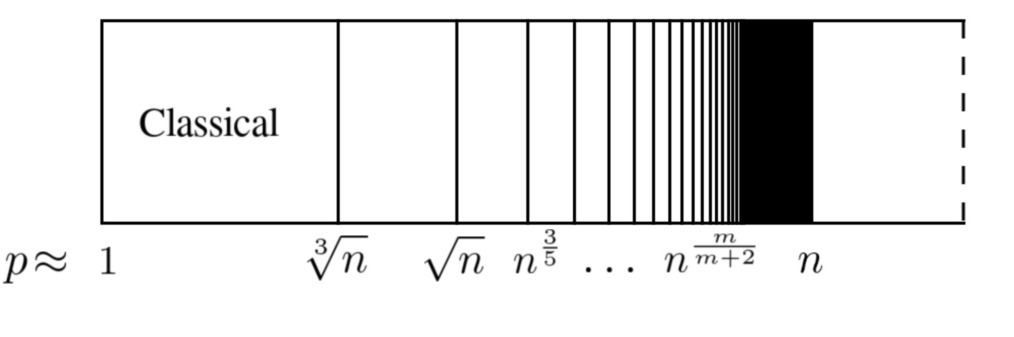 Figure 1
| Normalized empirical moment | Limit | Asymptotics of its squared error |
|---|---|---|
| 0 | ||
| 0 | ||
Peer Reviews
No public reviews on file for this paper yet. If you reviewed it on a platform where reviews are public (OpenReview, ICLR, NeurIPS, ICML), you can paste yours below so the community can read it here.
Videos
No videos yet. Explain this paper in a talk, walkthrough, or lecture? Add one.
The middle-scale asymptotics of Wishart matrices
Abstract
We study the behavior of a real -dimensional Wishart random matrix with degrees of freedom when but . We establish the existence of phase transitions when grows at the order for every , and derive expressions for approximating densities between every two phase transitions. To do this, we make use of a novel tool we call the G-transform of a distribution, which is closely related to the characteristic function. We also derive an extension of the -distribution to the real symmetric matrices, which naturally appears as the conjugate distribution to the Wishart under a G-transformation, and show its empirical spectral distribution obeys a semicircle law when . Finally, we discuss how the phase transitions of the Wishart distribution might originate from changes in rates of convergence of symmetric statistics.
60B20,
60B10,
60E10,
keywords:
[class=MSC]
Didier Chételat label=e1][email protected] Martin T. Wells label=e2][email protected]
1 Introduction
The roots of random matrix theory lies in statistics, with the work of Wishart (1928) and Bartlett (1933), and in numerical analysis, with the work of Von Neumann and Goldstine (1947). In this early period, many well-known matrix distributions were introduced. This includes the real Gaussian matrix ensemble , a matrix with independent standard Gaussian entries, the Gaussian orthogonal ensemble , the distribution of a symmetric matrix with , and the Wishart (also known as Laguerre) distribution , the distribution of a symmetric matrix with . During that time, the main concern was to derive properties of these distributions for a fixed dimension. Some asymptotics of the Wishart distribution were considered, but only as for fixed .
Starting with the pioneering work of Wigner (1951, 1955, 1957), Porter and Rosenzweig (1960), Gaudin (1961) and Mehta (1960a, b), researchers began investigating the asymptotics of Gaussian ensembles as their dimension grew to infinity. As a result of decades of work, the behavior of a matrix is now well understood both in the classical setting where is fixed, and in the setting where .
However, the situation asymptotics of the Wishart distribution is more complicated, as it depends on two parameters, and , and initial progress was slow. The work of Marchenko and Pastur (1967) clearly established that the analogue of a Gaussian orthogonal ensemble matrix whose dimension grows to infinity is a Wishart matrix whose degrees of freedom and dimension jointly grow to infinity in such a way that . Since then, we gained a very good understanding of the behavior of Wishart matrices in this regime.
But this body of work left open the question as to what happens to a Wishart matrix when with . Since such asymptotics are middle-scale between the classical regime where is fixed as and the high-dimensional regime where , we might refer to them as middle-scale regimes. Hence, we might ask: what is the asymptotic behavior of a Wishart matrix in the middle-scale regimes? This question is addressed this article.
To gain some intuition, it is instructive to look at the eigenvalues of a Wishart matrix. In the classical regime where is fixed as , the eigenvalues must all almost surely tend to by the strong law of large numbers. In constrast, in the high-dimensional regime where both with , the Marchenko-Pastur law states that for any bounded, continuous , {ceqn}
[TABLE]
where . Thus the eigenvalues do not all tend to , but rather distribute themselves in the shape of a Marchenko-Pastur law with parameter .
What happens between these two extremes? When , the Marchenko-Pastur law converges weakly to a Dirac measure with mass at . This suggests that whenever with {ceqn}
[TABLE]
or in other words that the eigenvalues converge almost surely to , as in the classical case.
This motivates a binary view of Wishart asymptotics. It appears that the behavior of a Wishart matrix in the middle-scale regimes is the same as in the classical regime, and therefore that there really are only two regimes: low-dimensional where , and high-dimensional where .
This binary view has very concrete repercussions. For example, in statistics, many covariance matrix estimators have been developed that leverage high-dimensional Wishart asymptotics (see Pourahmadi (2013) for a review). When faced with a problem where is large with respect to , it has been argued that the high-dimensional asymptotics, rather than the classical, constitute the correct model. The binary view provides a useful rule of thumb: small ’s call for classical covariance estimators, while large ’s call for high-dimensional covariance estimators.
Unfortunately, recent results establish that this binary view is incorrect. In the classical regime where is fixed, the central limit theorem implies that {ceqn}
[TABLE]
as , where the arrow stands for weak convergence. In fact, something better is known: recent work has extended this result to the case where tends to infinity. Recall that the total variation distance between two absolutely continuous distributions and with densities and is given by . With different approaches, Jiang and Li (2015) and Bubeck et al. (2016) independently established that {ceqn}
[TABLE]
whenever . Thus, when , the same asymptotics hold as in the fixed case, and we might regard these regimes as rightfully belonging to the classical setting.
The surprising part is that the converse is true! When , results of Bubeck et al. (2016) and Rácz and Richey (2016) show that {ceqn}
[TABLE]
Thus a phase transition occurs when is of the order . This begs the question: if a normal approximation fails to hold when grows faster than , what asymptotics hold? Is there a uniform asymptotic behavior that holds whenever with , or are there further phase transitions as the growth rate of is increased?
The results of this paper offers a mostly complete answer to this question. Namely, we establish that when but , {ceqn}
[TABLE]
where is a continuous distribution on the space of real symmetric matrices whose density is given when by
[TABLE]
for a . When grows like , another phase transition occurs. Namely, we establish that when but , {ceqn}
[TABLE]
where is a continuous distribution on the space of real symmetric matrices whose density is given when by
[TABLE]
again for a .
In general, for every we find a continuous distribution on the space of real symmetric matrices, with density given when by
[TABLE]
for a , which approximates the normalized Wishart distribution in some (but not all) middle-scale regimes. Namely, we prove the following, which can be regarded as the main result of this paper.
Theorem 1**.**
For any , the total variation distance between the the normalized Wishart distribution and the degree density satisfies {ceqn}
[TABLE]
as with .
The definition of and proof of Theorem 1 are found in Section 6, and follow from definitions and results from Sections 3, 4 and 5 that constitute the bulk of this paper.
The main consequence of this theorem is the existence of an infinite countable number of phase transitions, occurring when grows like for . A diagram is provided at Figure 1. This naturally groups the middle-scale regimes satisfying by which semi-open interval \big{[}\frac{K}{K+2},\frac{K+1}{K+3}\big{)} their limit belongs to. We might refer to this grouping as the degree of the regime. In other words, we will say an middle-scale regime satisfying has degree when \lim\limits_{n\rightarrow\infty}\frac{\log p}{\log n}\in\big{[}\frac{K}{K+2},\frac{K+1}{K+3}\big{)}.
The main result of this paper, Theorem 1, may then be summarized as saying that the normalized Wishart distribution can be approximated by the distribution with density in every middle-scale regime of degree or less. The degree case corresponds to the classical setting, while the higher degrees correspond to previously unknown behavior. In fact, we show that our degree approximation is asymptotically equivalent to the Gaussian orthogonal ensemble. The results of this paper can therefore be regarded as a wide generalization of the Wishart asymptotics results of Jiang and Li (2015), Bubeck et al. (2016); Bubeck and Ganguly (2016) and Rácz and Richey (2016).
Our approach relies on a novel technical tool we call the G-transform. It turns out that to understand middle-scale regime behavior of Wishart matrices, densities are less clear than characteristic functions (that is, Fourier transforms of densities). Unfortunately, characteristic functions are difficult to relate to metrics like the total variation distance. To remedy this problem, we develop the G-transform and some associated theory in Section 3. An interesting aspect of G-transform theory is that to every distribution we can associate a closely related distribution called its G-conjugate. In fact, the G-conjugate of a Wishart matrix is essentially a generalization of the distribution to real symmetric matrices. In Section 4, we define and derive several results concerning this new distribution, including a semicircle law. From these results, we derive in Section 5 approximations to the Wishart distribution for middle-scale regimes of every degree. Since these approximations are given using the language of G-transforms, we derive in Section 6 density approximations, from which Theorem 1 follows. We briefly discuss what concrete effects the phase transitions might have on Wishart asymptotics in Section 7. Finally, we compile auxiliary results in Section 8, while we discuss in Section 9 open questions that arise from these results.
Although the results of this paper explain a large part of the behavior of Wishart matrices when , there exists regimes for which yet for all , or in other words for which . An example is when grows at the order . Although the results of our paper characterize almost all middle-scale regimes in the sense that among those regimes satisfying , those such that represent a negligible set, they nonetheless exist. One might regard regimes such as those as having infinite degree. Beyond this, however, it is difficult to say anything about the behavior of Wishart matrices in these regimes. More work in that direction is clearly needed.
2 Notation and definitions
The transpose of a matrix is denoted t, and the identity matrix of dimension is . As is standard, we take the trace operator to have lower priority than the power operator: thus for a matrix , means the trace of . We will write when we mean the power of the trace of . The Kronecker delta is the symbol .
The space of all real-valued symmetric matrices is denoted . For a symmetric matrix , we define the symmetric differentiation operator by
[TABLE]
This operator has the elegant property that for any two symmetric matrices , .
The space of symmetric matrices can be assimilated to by mapping a symmetric matrix to its upper triangle. By integration over , we mean integration with respect to the pullback Lebesgue measure under this isomorphism, that is,
[TABLE]
We say a real symmetric matrix follows the Gaussian orthogonal ensemble distribution if , are all independent, with diagonal elements and off-diagonal elements .
Let be a matrix of i.i.d. random variables, and let be a positive-definite matrix. The Wishart distribution is the distribution of the random matrix . This is a special case of the matrix gamma distribution. Following Gupta and Nagar (1999, Section 3.6), we say a positive-definite matrix has a matrix gamma distribution with shape parameter and scale parameter if it has density over given by
[TABLE]
where is the multivariate gamma function. With this definition, the Wishart distribution is a matrix gamma with shape and scale .
While studying the Wishart distribution, the expression comes up so often that it makes sense to give it its own symbol. We will therefore write .
The Hellinger distance is metric between absolutely continuous probability measures. For two distributions and with densities and , their Hellinger distance is defined as
[TABLE]
The Hellinger distance is closely related to the total variation distance by the inequalities
[TABLE]
In particular, if and only if . Thus they can be seen as inducing the same topology on absolutely continuous probability measures, called the strong topology, in contrast to the topology induced by weak convergence of measures called the weak topology. One can show that if a sequence of measures converges in the strong sense (i.e. in the or metrics), then it converges weakly.
3 G-transforms
Our analysis of Wishart matrices relies heavily on a tool we call the G-transform of a probability measure. To do so, we first need to define the Fourier transform over symmetric matrices.
In Section 2, we clarified what we meant by integration over . For a function in , we define its Fourier transform to be
[TABLE]
It is more common to define the Fourier transform on symmetric matrices with the integrand \exp\big{\{}-i\sum_{k\leq l}T_{kl}X_{kl}\big{\}}, but choosing \exp\big{\{}i\operatorname{tr}(TX)\big{\}} considerably simplifies our computations.
We extend this definition to , in the usual manner. Because of the specific normalization chosen, this definition obeys a simple version of Plancherel’s theorem, namely
[TABLE]
We now define the G-transform. In itself, the definition has nothing to do with symmetric matrices and could have been perfectly well defined on any other space endowed with a Fourier transform.
Definition 1** (G-transform of a density).**
Let be an integrable function . Its G-transform is the complex-valued function defined by
[TABLE]
where stands for the principal branch of the complex logarithm.
In the same way that the Fourier transform maps to itself, the G-transform maps to itself.
By extension, for an absolutely continuous distribution on with density , we will define its G-transform to be the G-transform of its density. (This usage mirrors other transforms, such as the Stietjes transform.) We will usually denote the G-transform of by . Since a density is integrable, this is always well-defined. Moreover, , so the density can be recovered from the G-transform, and therefore to understand a distribution it is equivalent to study its density or its G-transform.
Two comments are in order. First, for many densities, . In this case, the G-transform can be written explicitly as
[TABLE]
Second, throughout this article we will often talk about “the” square root of a G-transform. To be clear, by we will always mean .
Now, in many ways, the G-transform behaves similarly to the characteristic function (Fourier transform of a density), but it has unique features. First, Plancherel’s theorem yields that
[TABLE]
Thus is itself a density, which we will call the G-conjugate of . (In particular, is much like a quantum-mechanical wavefunction.) We will also use an asterisk notation, so that the G-conjugate of a distribution will be denoted . For example, straightforward computations yield that , (where and are the univariate and distributions with degrees of freedom, respectively) and for any distribution and scalars , . Studying the G-conjugate of the Wishart distribution will play a key part in deriving results about the Wishart distribution itself. We should note that, in general, the double G-conjugate is not the same as . For example, is a density involving modified Bessel functions of the first kind, not a .
A second feature that distinguishes G-transforms from characteristic functions is that they are easy to relate to the Hellinger distance between probability measures. Consider two densities with G-transforms . By analogy, we could define the “total variation” and “Hellinger” distances of and by
[TABLE]
Since the modulus of the G-transforms integrate to one, their total variation and Hellinger distances are related to each other in the same way as in Equation 2.1 for densities, namely
[TABLE]
Thus if and only if . But the Hellinger distance between G-transforms is much more useful. Indeed, by the Plancherel theorem, for any two densities with G-transforms , their Hellinger distance satisfies
[TABLE]
Thus to compute the Hellinger distance between two densities, we can instead compute the Hellinger distance of their G-transforms. In contrast, there is no explicit way to express the Hellinger distance in terms of characteristic functions. And no such connection exists between the total variation distances of densities and G-transforms.
The G-transform does have some disadvantages compared to the Fourier transform. It is a non-linear transformation (and therefore not a true transform), and it does not behave well with respect to convolution. For our purposes, however, the advantages listed above outweigh these problems.
In practice, it is not aways easy to control the Hellinger distance directly, and one often focuses on the Kullback-Leibler divergence instead. The two quantities are related through the well known inequality
[TABLE]
For G-transforms, the following analog holds, which clarifies our interest in G-conjugates:
[TABLE]
where stands for the principal branch of the complex logarithm. In fact, in this article we will need a further generalization, where does not need to be a G-transform of a density.
Proposition 1** (Kullback-Leibler inequality for G-transforms).**
Let be the G-transform of an absolutely continuous distribution on , and let be an integrable function . Then
[TABLE]
for , where stands for the principal branch of the complex logarithm.
Proof.
We can write
[TABLE]
Now using the inequality that holds for any . The last quantity is bounded as
[TABLE]
In the second term, use for , while in the third term, use the Cauchy-Schwarz inequality to obtain
[TABLE]
Now use Jensen’s inequality in the second term and the algebraic identity in the third term to obtain
[TABLE]
as desired. ∎
Let us now compute the G-transform of the Gaussian Orthogonal Ensemble and the normalized Wishart distribution, which will be needed in our proofs. The density of a matrix over is
[TABLE]
To compute its G-transform, we will make use of the fact that the elements of a matrix are independent to reduce the expression to a product of characteristic functions.
Proposition 2**.**
The G-transform of the Gaussian Orthogonal Ensemble density on is
[TABLE]
Proof.
From Equation (3.9), is proportional to the density of the distribution, so it is integrable. Therefore, we can apply Equation (3.3) to find that
[TABLE]
for . The characteristic function of a is , so
[TABLE]
Squaring this result yields the desired expression for . ∎
In particular, we see that is the density of a distribution, or in other words that . In particular the Gaussian orthogonal ensemble is its own G-conjugate, up to a constant factor.
Let us now compute the G-transform of the normalized Wishart distribution. Unlike the case, the elements of the matrix are not independent, but the elements of its Cholesky decomposition are. By being careful about complex changes of variables, we can reduce the computation of the G-transform to the computation of characteristic functions of the Cholesky elements.
Proposition 3**.**
Let . Then the G-transform of the normalized Wishart distribution density on is given by
[TABLE]
Proof.
Recall the notation used throughout this article. The density of a distribution is
[TABLE]
If we do a change of variables , so that and
[TABLE]
we see that the normalized Wishart distribution has density
[TABLE]
Notice that is proportional to , so it must be proportional to the density of a matrix gamma distribution when , i.e. . In particular, it must be integrable. As was obtained by a linear change of variables from , must be integrable too, that is
[TABLE]
Therefore, we can apply Equation (3.3) to obtain
[TABLE]
If we rewrite the expectation in terms of , this last expression equals
[TABLE]
Since is real symmetric, there must be a spectral decomposition with real orthogonal and real diagonal. As has the same distribution as , namely , we can rewrite Equation (3.12) as
[TABLE]
Now, since is positive-definite it has a Cholesky decomposition with upper-triangular. According to Bartlett’s theorem (see Muirhead, 1982, Theorem 3.2.14), all the elements of are independent, the diagonal elements have the distribution and the upper diagonal elements have for . Since
[TABLE]
and , we have by independence and Equation (3.13) that
[TABLE]
We will now compute these expected values in several steps. For a given , let
[TABLE]
Since and , we have
[TABLE]
Consider the truncated integrands
[TABLE]
Clearly this sequence is dominated by the integrable positive function ,
[TABLE]
Therefore, by the Dominated Convergence Theorem and Equation (3.16),
[TABLE]
By the change of variables z=\big{(}\frac{n}{4}+\sqrt{n}D_{kk}i\big{)}x, this can be rewritten
[TABLE]
To compute this integral, we use a contour argument. Consider the closed path given by a path from [math] to , a path from to and finally a path from to 0. A diagram is provided as Figure 2.
As , is entire and its integral over must be zero. Therefore
[TABLE]
Do a change of variables , so that is real on the path. It yields
[TABLE]
This last integral is finite, since it is continuous on a bounded interval. Therefore the limit is zero and by Equation (3.17) and the previous expression,
[TABLE]
Going back to (3.14), let us now consider the expectations in the second products. For fixed , let
[TABLE]
Since
[TABLE]
Consider the truncated integrands
[TABLE]
We see that they are dominated by a positive, integrable function ,
[TABLE]
Therefore, by the Dominated Convergence Theorem and Equation (3.20), we conclude that
[TABLE]
A complex change of variables z=\big{(}\frac{n}{4}+i\sqrt{n}D_{kk}\big{)}x yields
[TABLE]
Let’s compute this integral again using a contour integration argument. Consider the contour given by a line from to , a line from to , a line from to and a line from to . A diagram is provided as Figure 3.
Since is holomorphic away from zero,
[TABLE]
By changes of variables and on the two respective integrals, we get
[TABLE]
Since \Big{|}\frac{n}{4}+y\sqrt{n}D_{kk}i\Big{|}^{-\frac{1}{2}}=\Big{(}\frac{n^{2}}{16}+y^{2}nD^{2}_{kk}\Big{)}^{-\frac{1}{4}} is continuous on , a bounded interval, we conclude that the integrals are finite and that the limits are zero. Therefore, by Equation (3.22),
[TABLE]
Recall the definitions of A and B at Equations (3.15) and (3.19). Combining both Equations (3.18) and (3.23) into the expression for at Equation (3.14) provides
[TABLE]
But by Muirhead (1982, Theorem 2.1.12),
[TABLE]
so by taking a factor out of the determinant, we find that
[TABLE]
Squaring this result yields the desired expression for . ∎
By Proposition 3, when the G-conjugate of a normalized Wishart distribution must have a density on given by
[TABLE]
As mentioned in the paragraph following Equation (3), the G-conjugate of a distribution is a scaled . Thus, by analogy, Equation (3.24) should be represent some kind of generalization of the distribution to the real symmetric matrices. Matrix-variate generalizations of the distribution have been investigated in the past, but not for symmetric matrices. Hence it appears the concept is new.
This motivates us to propose in Section 4 a candidate for a symmetric matrix variate distribution. Using that definition, the G-conjugate to the normalized Wishart could then be regarded as the distribution with degrees of freedom and scale matrix , which we denote . But regardless of its name, this distribution will play a key role in our results about the middle-scale regime asymptotics of Wishart matrices, and will be investigated in depth in Section 4.
4 The symmetric matrix variate distribution
In Section 3, Equation (3.24), we proved that when , the G-conjugate of the normalized Wishart distribution has density on given by
[TABLE]
Two remarks are in order. First, we are unaware of any matrix calculus tools that could let us integrate this expression directly. Thus, the mere fact that this expression integrates to unity, a consequence of being the G-conjugate of another distribution, seems remarkable.
Second, when , this is the distribution. Thus, as we mentioned while discussing Equation (3.24), it is natural to interpret this distribution as the parametrization of some generalization of the distribution to , the space of real-valued symmetric matrices. The purpose of this section is to propose a candidate definition for such generalization, as well as prove several results concerning the normalized Wishart G-conjugate.
To the best of our knowledge, no extension of the distribution to symmetric matrices has ever been proposed. However, a non-symmetric matrix variate distribution has been thoroughly investigated in the literature – see Gupta and Nagar (1999, Chapter 4) for a thorough summary. Several definitions exist. For our purposes, we say that a real-valued random matrix has the matrix variate distribution with degrees of freedom and positive-definite scale matrix if it has density
[TABLE]
It is not exactly clear what should be the proper analog of this distribution for symmetric matrices. But it would be elegant if the degrees of freedom of Equation (4.1) were to be exactly , as in the univariate case. Thus, the following definition seems natural.
Definition 2** (Symmetric matrix variate distribution).**
We say a real symmetric matrix has the symmetric matrix variate distribution with degrees of freedom and positive-definite scale matrix , denoted , if it has density
[TABLE]
With this definition, the G-conjugate to the normalized Wishart distribution, whose density is given by Equation (4.1), is the distribution on .
In fact, since Equation (4.1) integrates to one, we can deduce the normalization constant of Definition 2. For an arbitrary degrees of freedom parameter , imagine the density of the G-conjugate of a normalized Wishart distribution with . By virtue of being a G-conjugate, it must integrate to unity. Then from the change of variables which has Jacobian , we see that
[TABLE]
Thus we must have
[TABLE]
It would be interesting to see if this distribution satisfies the properties we would expect of a distribution, to ensure our guess is the “correct” one. However, this would take us too far away from the topic of this article. Instead, we will focus in the rest of this section on proving results about , the G-conjugate to the normalized Wishart distribution.
Our first result will concern the asymptotic expansion of its normalization constant. We mention that this constant is the same as the term appearing in the expression of the G-transform of the normalized Wishart in Proposition 3.
Lemma 1**.**
The normalization constant of the distribution
[TABLE]
has, for every , the asymptotic expansion
[TABLE]
as with .
Proof.
By Stirling’s approximation applied to , as well as Muirhead (1982, Theorem 2.1.12), we find that
[TABLE]
as . Thus
[TABLE]
as with , and so by Equation (4.3),
[TABLE]
Let us now focus on the two sums in this expression. Recall that for any ,
[TABLE]
even for negative . Therefore,
[TABLE]
Now let denote the Bernoulli numbers, with the convention . Faulhaber’s formula provides
[TABLE]
But by the binomial theorem, , and for any . Thus
[TABLE]
Using that and , we obtain
[TABLE]
The analysis of the other sum of Equation (4.4) is similar but more involved, as we must distinguish the cases where is even and where is odd. We find, from Equation (4.5) again, that
[TABLE]
At this point, it is simpler to analyze the cases where is even and odd separately. If is odd, define and observe that by Faulhaber’s formula,
[TABLE]
By the binomial theorem, , and for . Moreover,
[TABLE]
and
[TABLE]
Thus, for odd , Equation 4.7 equals
[TABLE]
Moreover,
[TABLE]
Thus,
[TABLE]
When is even, let and observe that by Faulhaber’s formula,
[TABLE]
But by the binomial theorem, , and for . If we apply Equations (4.8)–(4.9), then Equation (4.7) becomes
[TABLE]
Moreover,
[TABLE]
Thus again,
[TABLE]
which is the exact same result as in the odd case (see Equation 4.10). Plugging Equations (4.6) and (4.10)–(4.11) in Equation (4.4), we obtain
[TABLE]
as desired. ∎
Thus the constant is closely related to the normalization constant of the distribution .
We now turn our attention to the study of the asymptotic moments of a distribution. We first remind the reader of some classic results. For a Gaussian Orthogonal Ensemble matrix , a moment-based approach to Wigner’s theorem states that for any , its moment satisfy
[TABLE]
where is the Catalan number. In fact, Anderson et al. (2010, section 2.1.4 on p.17) show that the variance of the moment satisfies \lim\limits_{p\rightarrow\infty}\text{Var}\big{[}\frac{1}{p}\operatorname{tr}(Z/\sqrt{p})^{k}\big{]}=0, so we really have
[TABLE]
as .
Now, what do we know about the moments of ? By symmetry, for odd , but it is much less clear what happens for even . It turns out that in many ways, if then mimics the Gaussian Orthogonal Ensemble results outlined above, especially when as . We have the following result.
Theorem 2**.**
Let and . If , the moments of satisfy the asymptotic bounds and as . In fact, for any ,
[TABLE]
as with , where is the Catalan number.
Although our proof will rely on the close relationship between the Wishart and the distribution, it is worthwhile to step back and think why a should behave like a when . One good reason might be the classic result that as , the density of a distribution converges pointwise to a standard normal density. Thus, we might think that as long as does not grow too fast, in some aspects the symmetric distribution should behave like a .
In the context of the proof, it will prove useful to use the notion of power sum symmetric polynomials. For any integer partition in decreasing order , define its associated power sum polynomial to be
[TABLE]
The norm of the partition is , which should not be confused with its length (number of elements).
By convention, we will assume there also exists an empty partition with length , norm and power sum polynomial .
Let’s now turn to the proof of the theorem. The odd moments of the moments are zero by symmetry, so it makes sense to focus on the even moments and the square moments . Our first step in the proof is to express these in terms of expectations of power sum polynomials of an inverse Wishart , where by power sum polynomials we mean expressions like at Equation (4.12). Recall the useful shorthand .
Lemma 2**.**
Let . Then for any , whenever is large enough so that , we can compute the moment of by
[TABLE]
and its squared moment by
[TABLE]
for and some , . These , are polynomials in , indexed by integer partitions , whose degrees satisfy and . The sums are taken over all partitions of the integers satisfying and respectively, including the empty partition.
Proof.
Let and stand for the density and the G-transform of a normalized Wishart matrix . In the proof of Proposition 3, we concluded at Equation (3.11) that had to be integrable when , as its integral was proportional to a multivariate gamma function. Let be the flip operator. Since is integrable, must be integrable as well, and so their convolution f^{1/2}_{\text{NW}}\star\big{(}f^{1/2}_{\text{NW}}\circ R\big{)} is well-defined and integrable.
At Equation (3.1) at the start of Section 3, we defined our notion of Fourier transform for integrable functions on . Define the map that maps a symmetric matrix to its vectorized upper triangle, and let be the map
[TABLE]
Then in terms of the usual Fourier transform on ,
[TABLE]
This close relationship transfer properties to our Fourier transform on . We will need three.
For any integrable function , we have \mathcal{F}\big{\{}\overline{f\circ R}\big{\}}=\overline{\mathcal{F}\{f\}}. 2. 2.
(Convolution) For any two integrable functions and , we have . 3. 3.
(Fourier inversion) For any continuous integrable with integrable Fourier transform , we have
[TABLE]
for all .
These properties are important for the following. Since is real-valued, properties 1 and 2 provide
[TABLE]
But then, since is integrable (in fact, to unity), the Fourier inversion formula yields that
[TABLE]
Thus we might say the characteristic function of the distribution is given by f^{1/2}_{\text{NW}}\star\big{(}f^{1/2}_{\text{NW}}\circ R\big{)}. It is well known that the derivatives of the characteristic function of a distribution evaluated at zero provide its moments, up to a constant. This suggests we should try to repeatedly differentiate f^{1/2}_{\text{NW}}\star\big{(}f^{1/2}_{\text{NW}}\circ R\big{)} at zero to compute and , our ultimate goal.
Unfortunately, the convolution is given by an integral whose domain makes it difficult to directly interchange the differentiation and integration symbols. Because the integrand is orthogonally invariant, we found it easier to compute the derivatives at zero by taking a limit over a sequence of decreasing positive-definite matrices at both sides instead. In this spirit, define on the open set the real-valued functions
[TABLE]
and
[TABLE]
for fixed , and . Here stands for the symmetric differentiation operator , as defined in Section 2. The scaling in the argument helps link the convolution to an expectation with respect to an inverse Wishart distribution.
Let’s first relate these functions to the moments of the distribution. The symmetric differentation operator has the pleasant property that for any two symmetric matrices , . Thus, for any and indices , we find that
[TABLE]
for all .
We now show that the right hand side (4.15) is integrable. This is not a mere formality: when , asking if this expression is integrable is the same as asking if the distribution with degrees of freedom has an moment, and it is well-known that the distribution only possesses moments of order smaller than its degrees of freedom. So the answer is most likely to be positive, but only for large enough.
Let us see why. For any symmetric matrix ,
[TABLE]
where are the ordered eigenvalues of the positive-definite matrix . Thus
[TABLE]
When , the last integrand is the density of a distribution, so integrates to unity. Thus, when , the right hand side of Equation (4.16) is an integrable function for all and . By Equation (4.15), and repeated differentiation under the integral sign justified by the integrability bounds given by Equations (4.16) and (4.17), we find that
[TABLE]
and
[TABLE]
for any and any .
Now let’s relate and to the definition of f^{1/2}_{\text{NW}}\!\star\!\big{(}f^{1/2}_{\text{NW}}\!\circ\!R\big{)} as a convolution. This is where restricting and to small positive-definite matrices becomes useful. By Equation (3.10), the expression is
[TABLE]
using the change of variables with . For , we have , and thus , satisfy
[TABLE]
and
[TABLE]
We would now like to interchange the integral and differentiation signs. To do so, we must understand what the repeated derivatives of \exp\{-\frac{n}{4}\operatorname{tr}Y\Big{\}}|Y|^{\frac{m}{4}} look like. Differentiating once, we see that:
[TABLE]
Differentiating twice, we see that:
[TABLE]
So in general, it is clear that the repeated derivatives are given by some polynomial in entries of , times \exp\{-\frac{n}{4}\operatorname{tr}(Y+X)\Big{\}}|Y+X|^{\frac{m}{4}}. We won’t investigate further the nature of these polynomials beyond remarking that for any indices and , and any symmetric matrices , we must have some crude bound
[TABLE]
for some polynomials that do not depend on or . We relegate a proof of this result as Lemma 3 in Section 8. This can be uniformly bounded for all by
[TABLE]
for some constant that does not depend on or . But for any and ,
[TABLE]
for a with a matrix gamma distribution . The Cauchy-Schwarz inequality then entails the bound
[TABLE]
The first expectation is always finite when . Since can be written as a sum of zonal polynomials indexed by partitions of the integer , the results of Muirhead (1982, Theorem 7.2.13) imply that the second expectation is finite whenever . Thus, in Equation (4.20) with and (4.21) with , whenever we are justified in repeatedly differentiating under the integral sign by the integrability bounds given by Equations (4.22) and (4.23), and obtain in that case
[TABLE]
and
[TABLE]
Let us now look at how and behave as . On one hand, for any symmetric matrix we have , so we must have the bounds
[TABLE]
and
[TABLE]
holding uniformly in . When , the right hand sides are proportional to the density of the G-conjugates of the normalized Wishart distributions with degrees of freedom, so are integrable. Thus, by the dominated convergence theorem and Equations (4.18) and (4.19),
[TABLE]
and
[TABLE]
for .
On the other hand, the integrands at Equations (4.25) and (4.26) take a particularly simple form. Lemma 4 establishes by induction that there must be polynomials and in , and with degrees and such that
[TABLE]
and
[TABLE]
for any and . The sums are taken over all partitions of the integers satisfying and respectively, including the empty partition. But for any integer partition , the bound
[TABLE]
holds uniformly in . Thus for , the right hand side is integrable for , by the same argument as for Equation (4.23). Thus for such , by the dominated convergence theorem and Equations (4.29) and (4.30), we obtain that
[TABLE]
and
[TABLE]
where follows a distribution. Combining Equations (4.27)–(4.28) with Equations (4.31)–(4.32) and Lemma 4 concludes the proof. ∎
Something remarkable about Lemma 2 is that it provides us with an algorithm to compute the moments of a symmetric distribution in terms of the moments of an inverse Wishart matrix. For example, when , repeated differentiation yields that
[TABLE]
We can recognize and as the power sum polynomials and in the sense of Equation (4.12), so we must have , , and in the result of Lemma 4. Hence Lemma 2 really tells us that whenever , for can be expressed as
[TABLE]
where .
Of course, this also works with square moments and higher . For example, the same strategy for, say, square moments with yields that whenever , for can be expressed as
[TABLE]
again where .
Unfortunately, as we consider larger orders, the repeated differentiation of quickly becomes too cumbersome to perform by hand. But at least in theory, we can compute expressions like (4.34) and (4.35) for any and , and Lemma 2 summarize that fact. That is, using the Fourier inversion theorem we have reduced the problem of computing moments of the -distribution to that of computing expected power sum polynomials of the inverse Wishart distribution , for large enough .
How can we compute expected power sum polynomials of an inverse Wishart? There are two approaches in the literature. Letac and Massam (2004) found an expression in terms of a different basis, the zonal polynomials, which behave particularly nicely with respect to the inverse Wishart distribution, and whose expectations have a simple closed form. From this, they provided an algorithm for computing expected power sum polynomials to arbitrary order. Matsumoto (2012) found expressions of coordinate-wise moments in terms of modified Wiengarten orthogonal functions, from which expectations of power sum polynomials can be computed. We follow the idea of Letac and Massam (2004) in our asymptotic analysis.
For any integer partition , there exist coefficients (which depend solely on and ) such that
[TABLE]
for the so-called zonal polynomials. For an overview of the topic with a focus on random matrix theory, see Muirhead (1982, Chapter 7). The coefficients are explicitly computable. If we follow the normalization of zonal polynomials of Muirhead (1982), for example, we find that
[TABLE]
As mentioned, expectations of zonal polynomials with respect to a Wishart or inverse Wishart distribution take a particularly simple form. From Muirhead (1982, Theorem 7.2.13 and Equation (18) on p.237), the expected zonal polynomials for are
[TABLE]
for , and . For example, the first few expected zonal polynomials are
[TABLE]
From this, we can exactly compute and thus and , as a function of and (or ). For example, by Equation (4.38) we find that
[TABLE]
and thus, by Equation (4.34), whenever
[TABLE]
In a similar way, we can compute the expected zonal polynomials and hence, the expected power sum polynomials of for . So from Equation (4.35), we obtain for that
[TABLE]
Of course, this reasoning also works for other ’s. In particular, we essentially derived a (potentially inefficient) algorithm to compute the moments of a distribution to arbitrary order on our path to proving this theorem.
At this point, it is worthwhile to realize that Equations (4.40) and (4.41) are already enough to prove the theorem for small moments. For example, when such that , then and
[TABLE]
which proves that . In fact,
[TABLE]
Moreover, when such that , then and
[TABLE]
Thus {ceqn}
[TABLE]
and the theorem is proven for the second moment.
In theory, we could proceed in the same way for any moment of interest, but naturally we could never conclude that the theorem holds for all moments that way. Nonetheless, the calculations give us some hints about how to argue in the general case.
The idea is to express the moments of the symmetric distribution as polynomials of and . There are two regimes where random matrix theory is well understood: the classical regime where is held fixed as , and the linear, high-dimensional regime where grows linearly with . From this, we can therefore conclude a few facts regarding the behavior of symmetric moments in these regimes. But these moments are polynomials, and a polynomial is a very rigid object: results from the two extreme cases where is fixed and grows linearly will be enough to prove results for every regime in between, yielding the first part of the theorem. Proving the second part will then be the simple matter of applying the GOE approximation of Jiang and Li (2015) and Bubeck et al. (2016) to the specific shape found for the symmetric moments while proving the first part, namely Equations (4.58) and (4.59).
Proof of Theorem 2.
Recall the expected zonal polynomial of an inverse Wishart is given by Equation (4.39). Based on the previous calculations, it is tempting to define
[TABLE]
so that {ceqn}
[TABLE]
With these expressions the expected power sum polynomials can be written as
[TABLE]
In other words, if we define
[TABLE]
then
[TABLE]
But R^{-1}_{\mu}(m)=\prod_{i=1}^{q(\lambda)}\prod_{l=0}^{\lambda_{i}-1}\big{(}1-\frac{1-i+2l}{m}\big{)} is a polynomial in , while is a polynomial in and , both of degree at most . Thus
[TABLE]
for some coefficients that don’t depend on , (or ). Define the polynomials , so that
[TABLE]
Let us show that for all , the polynomial must be identically zero over the interval \alpha\in\big{(}0,1/\max(|\kappa|-2,0)\big{)}. Indeed, say this was not the case, and let be the smallest with the property that for some \alpha_{0}\in\big{(}0,\frac{1}{\max(|\kappa|-2,0)}\big{)}. As is a polynomial, by continuity it must be non-zero in a neighborhood of , so we may as well assume is rational without loss of generality. Now look at what happens to as grows to infinity at the very specific linear rate . Since is rational, there must be a subsequence such that is exactly an integer (for example, if with , integers, we can take ). Then for , we have exactly .
Since , then |\kappa|<1+\big{(}\frac{\alpha_{0}}{1+\alpha_{0}}\big{)}^{-1}. Thus by Hölder’s inequality and Lemma 5,
[TABLE]
On the other hand, by Equations (4.46) and (4.48), the definition of and the fact that as ,
[TABLE]
As , must therefore equal zero, a contradiction. Hence, as claimed, the polynomials for all vanish over the interval \big{(}0,\frac{1}{\max(|\kappa|-2,0)}\big{)}.
But a polynomial can have an infinite number of zeros only if all its coefficients are zero, so we conclude that {ceqn}
[TABLE]
Thus, from Equations (4.46) and (4.47) we have
[TABLE]
where
[TABLE]
Going back to equations (4.13) and (4.14) and plugging in the above yields that as long as ,
[TABLE]
where
[TABLE]
Now, for any , we can associate a partition of norm with the partition of norm , which satisfies
[TABLE]
By definition for the ’s at Equation (4.44), this means that every factor that appears in appears in , so by definition of the ’s at Equation (4.45), is a polynomial in . Moreover, as and are polynomials of degrees and respectively, there exists coefficients and such that
[TABLE]
and
[TABLE]
As in the first case and in the second case, we conclude that these two expressions are polynomials in and . Therefore, looking back at (4.49) and (4.50), we conclude that the ’s and ’s are polynomials in and . Therefore, if there must be coefficients , and large enough integers , such that
[TABLE]
for polynomials and .
We will now proceed to show that and must vanish on for and respectively. Our argument relies on the analysis of the asymptotic behavior of the moments of in the classical regime where is held fixed while grows to infinity.
Observe first that and must have a finite limit as with held fixed. Indeed, since is positive definite, is greater than one and so we have the bound
[TABLE]
When is held fixed, by Lemma 1. Moreover,
[TABLE]
for the eigenvalues of , and is monotone decreasing towards . Therefore, for a fixed dimension we can apply the monotone convergence theorem to obtain that
[TABLE]
for . Repeating the argument with yields similarly
[TABLE]
Thus indeed and have finite limits when is held fixed.
We can use this to show that and must vanish on for and as follows. Say the first statement wasn’t true, and let be the smallest such that for some , . Then by Equation (4.51) and the definition of , the limit of as with fixed at satisfies
[TABLE]
But tends to infinity as tends to infinity, and since , Equation (4.53) means that must tend to zero. Thus has to equal zero, which contradicts our assumption. Thus for every , the polynomial must vanish on .
Similarly, for , the polynomial must vanish on , because if it wasn’t the case, we could take as the smallest with the property that for some , , and then by Equation (4.52) with fixed at as we would get
[TABLE]
But then by Equation (4.54), as tends to infinity and the ratio must tend to zero. Thus we must have , a contradiction. Hence indeed for , the polynomial must vanish on .
But of course, a polynomial can only have an infinite number of zeroes if its coefficients are all zero, so we must have {ceqn}
[TABLE]
Now say that varies with in such a way that . Then for large enough , so by Equations (4.51) and (4.57),
[TABLE]
and by Equations (4.52) and (4.57),
[TABLE]
Although we might not know what coefficients are, this shows at least that the limits are finite. In particular, from Equations (4.58) and (4.59) we can conclude that and , which shows the first claim of the theorem.
For the second claim, let with . Then Equations (4.58) and (4.59) specialize to {ceqn}
[TABLE]
What is interesting about this result is that these limits must be the same regardless of the way grows! As long as with , the limits are and , regardless of whether or or some other growth.
Now, Bubeck et al. (2016, Theorem 7) and Jiang and Li (2015, Theorem 1) have shown that when with , the total variation distance between a normalized Wishart matrix and a Gaussian Orthogonal Ensemble matrix tends to zero as . Therefore, the Hellinger distance satisfies also as .
But convergence in Hellinger distance has strong implications for real-valued statistics. Indeed, for , and any function such that , are square-integrable,
[TABLE]
by the Cauchy-Schwarz inequality.
Let’s consider applying this result to and . What do we know about these statistics? In the case where , results of Anderson et al. (2010, Lemma 2.1.6 and the equation above Equation (2.1.21)) provide that
[TABLE]
because these expressions only depend on , and since as , taking a limit as is the same as taking a limit as . Moreover, in the case, using Jensen’s inequality and Equations (4.58)–(4.59) we can at least see that
[TABLE]
Therefore, using Equation (4.63) with and we find that when with ,
[TABLE]
Since implies , we conclude from Equation (4.62) that {ceqn}
[TABLE]
But then, by that same equation, we conclude that when , not only when but for all such that , we have {ceqn}
[TABLE]
for . To finish the proof, use Equation (4.66) with the fact that for odd to find that
[TABLE]
Thus , as desired. This proves the second claim and concludes the proof. ∎
A pleasant consequence of this result is that when with , we can conclude a version of the semicircle law holds for the distribution. This is interesting because the distribution has dependent entries with heavy tails, whose distribution varies with .
Let , with eigenvalues . Then define its empirical spectral measure to be {ceqn}
[TABLE]
Since depends on the random matrix , it is a random measure on .
Corollary 1** (Semicircle law for the distribution).**
The empirical spectral measure of a random matrix converges weakly, in square mean, to the semicircle distribution {ceqn}
[TABLE]
Proof.
Let be any continuous function that vanishes at infinity. By the Stone-Weierstrass theorem, there exists a sequence of polynomials such that for any , . To fix some notation, write
[TABLE]
Then since and are both probability measures,
[TABLE]
By Theorem 2, the expectation tends to zero as with . Thus
[TABLE]
But this is true for every , so the limit must be zero. Hence for every continuous that vanishes at infinity, the integral converges in square mean to . By Chung (2001, Theorem 4.4.1 and 4.4.2), this implies that for every bounded continuous , the integral converges in square mean to . Thus the empirical spectral distribution converges weakly, in square mean, to the semicircle distribution , as desired. ∎
5 Wishart asymptotics: the G-transform point-of-view
We now turn our attention to the main objective of this paper, namely studying the behavior of Wishart matrices in the various middle-scale regimes. To do this, we exploit the close connection between the Wishart and the symmetric distributions and make use of the results found Section 4. The main result of this section, Theorem 3, states that we can approximate for every middle-scale regime the G-transform of a normalized Wishart by a degree-specific function . This can be seen as an analogue of Theorem 1 in the G-transform domain.
The reasoning behind the approximations is as follows. We could imagine writing from Proposition 3 in exponential form, and expanding the terms as a Taylor series would yield
[TABLE]
Now imagine that the ’s appearing in the expression follow a distribution. By Theorem 2, we know that \operatorname{tr}\big{(}\frac{4T}{\sqrt{p}}\big{)}^{k}=\Theta(p) when is even, in an sense. When is odd, the theorem merely proves that \operatorname{tr}\big{(}\frac{4T}{\sqrt{p}}\big{)}^{k}=o(p), but for a matrix , we know that is asymptotically normal for odd by Anderson et al. (2010, Theorem 2.1.31). This would suggest that \operatorname{tr}\big{(}\frac{4T}{\sqrt{p}}\big{)}^{k}=\Theta(1) when is odd. Thus we would have, in some sense,
[TABLE]
In other words, terms in the power series would be associated with some degree , such that they would be non-negligible in any middle-scale regime of degree up to , and negligible in higher degrees. In fact, a similar phenomenon occurs with , by Lemma 1. This suggests we should try truncating these power series to derive degree-specific approximations.
Definition 3** (G-transform approximations).**
For any , define the degree approximation as
[TABLE]
Just like the G-transform of a normalized Wishart matrix, these functions implicitly depend on . The first three are
[TABLE]
These functions have the pleasant property that their modulus is bounded, up to a constant, by the G-conjugate density . Indeed, on one hand we can rewrite Definition 3 into
[TABLE]
On the other hand, for any , we can write 1+ix=\sqrt{1+x^{2}}\exp\big{(}i\;\text{atan}(x)\big{)} with the arctangent function taking values in . Thus by Proposition 3 we can rewrite as
[TABLE]
with the understanding that the matrix-variate arctangent function operates on eigenvalues by functional calculus. Now, for any and odd integer , there is an elementary inequality
[TABLE]
Notice that is always an odd integer. Thus, from the above inequality and Equations (5.1) and (5.2), we can derive the bound
[TABLE]
In particular, since is integrable whenever by Proposition 3, Equation (5.3) implies that every must also be integrable whenever . In particular, for large enough it makes sense to talk about the asymptotic total variation or Hellinger distance between and .
We now state the main result, which is that each function approximates the G-transform of a normalized Wishart for all middle-scale regimes of degree or lower, but no other.
Theorem 3**.**
Let as . For any , the total variation distance between the G-transform of the normalized Wishart distribution and the approximating function satisfies
[TABLE]
if and only if .
Proof.
If statement. For the first part of the theorem, remark that by Equation (3.7) it is equivalent to show that the Hellinger distance tends to zero, i.e. that
[TABLE]
when . To control this quantity, we use the Kullback-Leibler inequality for G-transforms. Notice that for any and ,
[TABLE]
Let stand for the principal branch of the complex logarithm, and let us study . Its real part can be bounded by
[TABLE]
By Equation (5.4), this can be bounded by
[TABLE]
We can bound the imaginary part of in a similar way. Define to be the projection mapping . A plot is given as Figure 4.
It satisfies for all branches of , as well as the inequality . Using this mapping, we can see that the imaginary part of can be bounded as
[TABLE]
By Equation (5.5), this can be bounded by
[TABLE]
Recall that the G-conjugate of the normalized Wishart distribution is the distribution with degrees of freedom and scale matrix , denoted – see Equation (3.24) and Section 4 for details. Let us bound the expectations of these absolute real and imaginary parts under this distribution. By Equations (5.10), (5.6), (5.7) and Theorem 2, we find that for ,
[TABLE]
and
[TABLE]
as with .
Moreover, from Lemma 1, we see that
[TABLE]
Thus, from Equations (5.3) and (5.10), we see that when , the asymptotic norm of is bounded by
[TABLE]
In fact, at the end of this proof we will see that this bound is sharp and the limit must be exactly 1.
Using Equations (5.8), (5.9) and (5.11) with Proposition (1) implies that when ,
[TABLE]
Thus \mathrm{H}^{2}\big{(}\psi_{\text{NW}},\psi_{K}\big{)}\rightarrow 0, hence by Equation (3.7) we must have the limit \mathrm{d}_{\text{TV}}\big{(}\psi_{\text{NW}},\psi_{K}\big{)}\rightarrow 0, as desired.
Only if statement. For the second part of the theorem, assume that the total variation distance satisfies , hence \mathrm{H}\big{(}\psi_{\text{NW}},\psi_{K}\big{)}\rightarrow 0 by Equation (3.7), as . We will show by contradiction this implies that .
Assume this wasn’t the case. Since , there must be an such that , and since , we must have . By Equation (5.8), we must have for that
[TABLE]
so
[TABLE]
Now write, by Equation (5.1) and Definition 3,
[TABLE]
But as , we must have , so by Theorem 2, we have . Moreover, as we assumed that , we must have . Thus
[TABLE]
Then by the reverse triangle inequality,
[TABLE]
for a , that is
[TABLE]
Since convergence implies convergence in probability, by the continuous mapping theorem we must have
[TABLE]
as , so by Equation (5.12)
[TABLE]
But then, from Equation (5.13) and Slutsky’s lemma (van der Vaart, 2000, Lemma 2.8 (iii)),
[TABLE]
as . As is deterministic, this implies that as , a contradiction. Thus whenever \mathrm{H}^{2}\big{(}\psi_{\text{NW}},\psi_{K}\big{)}\rightarrow 0 as with , we must have , as desired. This concludes the proof. ∎
Although Theorem 3 states that the functions approximate , there is no guarantee that they are G-transforms of a probability density. In other words, nothing guarantees that their inverse G-transforms are real-valued, non-negative and integrate to unity. However, the reverse triangle inequality applied to the -norm provides that
[TABLE]
so Theorem 3 and the Plancherel theorem implies that
[TABLE]
when . That is, the theorem at least guarantees that is asymptotically a density in its associated regime. We discuss this further in Section 6.
We independently know, by the results of Jiang and Li (2015) and Bubeck et al. (2016), that a Gaussian orthogonal ensemble approximation holds in the classical regime. Although is not the G-transform of a , a simple Kullback-Leibler argument is sufficient to prove that it approximates for degree regimes.
Proposition 4**.**
The total variation distance between the degree G-transform approximation and the Gaussian orthogonal ensemble G-transform satisfies as with .
Proof.
We use a similar strategy to Theorem 3: namely, by Equation (3.7) is it equivalent to prove that as with , and to control that quantity we can use the Kullback-Leibler inequality for G-transforms.
Let . Since the Gaussian orthogonal ensemble has been extensively studied, we understand well its empirical moments. For example, according to Anderson et al. (2010, Lemma 2.2.2), we have , while from Equation (2.1.45) of the same book we have and . Then from Definition 3 and Proposition 2, and using the projection map as in the proof of Theorem 3, we find that
[TABLE]
and
[TABLE]
Since when with by Equation (5.14), if we apply Proposition 1 we find thatt
[TABLE]
for . By Equation (3.7), this concludes the proof. ∎
As a consequence, when with by Theorem 3 and Proposition 4. Hence by Equation (2.1) in the classical setting. This provides an alternative proof of the results of Jiang and Li (2015) and Bubeck et al. (2016).
6 Wishart asymptotics: the density point-of-view
In Section 5, we studied the asymptotic behavior of the normalized Wishart distribution using its G-transform . In particular, we derived an approximation to for every middle-scale regime of a given degree. But although it is equivalent to study a probability distribution from a density or a G-transform point of view, it is still natural to wonder if we can find approximations to the density of a normalized Wishart for every middle-scale regime of a given degree.
Recall from Theorem 3 that when . Define . In general, there is no guarantee that these should be real-valued. On the other hand, we know from Equation (5.3) that whenever , must be integrable, and since the G-transform maps integrable functions to integrable functions, must also be integrable. In fact, according to Equation (5.14), we know must be asymptotically a density when . This suggests we define the following densities.
Definition 4** (Density approximations).**
For any and , define the degree density approximation as {ceqn}
[TABLE]
where and is as in Definition 3. The distribution on the real symmetric matrices with density will be denoted .
The main interest is that we can asymptotically approximate the density of a normalized Wishart by the bona fide densities . This was the content of Theorem 1 from Section 1, which we now prove as a simple corollary of its G-transform analogue Theorem 3 from Section 5.
Proof of Theorem 1.
As in the rest of this paper, we write the density of the normalized Wishart distribution by , and by Definition 4 the density of is . Notice that by Equation (2.1), to prove it is equivalent to prove that . From the triangle inequality, the reverse triangle inequality, Theorem 3 and Equation (5.14),
[TABLE]
when . Thus , hence , tends to zero when with , as desired. ∎
We defined in terms of the inverse G-transform of the functions given by Definition 3. How can we express this explicitely? By Equation (5.3), we see that is asymptotically bounded by the density , which is integrable whenever . But is proportional to a density in the sense of Definition 2, which is integrable for , that is whenever . Thus and therefore is integrable whenever . Hence we can use the Fourer inversion theorem to conclude that is proportional to the integral
[TABLE]
whenever . In particular, if we do a change of variables , we obtain Equation (1.3) from Section 1 whenever , from which we can derive Equations (1.1) and (1.2).
It would be quite pleasant if there was a way to solve the integral in Equation (6.1) or (1.3) and obtain a (potentially quite complicated) closed form expression for up to its normalization constant. So far, our efforts have been unfruitful.
We close our discussion with a final remark. At the end of Section 5, we showed that approximates in degree middle-scale regimes, from which the classical asymptotic normality follows. It is natural to wonder if approximates in the same context. An argument similar to that of Theorem 1 shows this is the case.
Proposition 5**.**
The total variation distance between the degree density approximation and the Gaussian orthogonal ensemble G-transform satisfies as with .
Proof.
The Hellinger distance between and satisfies
[TABLE]
By Equation (2.1), the result follows. ∎
Of course, we could conclude from this that when with , offering yet again another proof that a Gaussian orthogonal ensemble approximation holds in the classical setting.
7 The effect of phase transitions
Although we have established the existence of phase transitions, it does not shed much light on how the behavior of a normalized Wishart distribution might differ across phase transitions. To do this, it can be very illuminating to study the asymptotics of some of its statistics. For example, we could study its empirical moments.
For a normalized Wishart matrix , a direct computation yields
[TABLE]
so in every middle-scale regime, that is whenever with ,
[TABLE]
Thus we have convergence of the second empirical moment to , but otherwise nothing very interesting. There doesn’t seem to be any change of behavior across the different middle-scale regimes. In contrast, the situation with the symmetric distribution is striking, and illustrates yet again that middle-scale regime behavior becomes clearer under a G-transform. Indeed, we know from Theorem 2 that for a , the quantity also converges to 1, but we know more. At Equation (4.43), we computed the exact distance between and , and found that
[TABLE]
Thus the distance must have middle-scale asymptotics
[TABLE]
as with . Thus there is a sharp change in behavior of when grows like , and despite the symmetric distribution satisfying a semicircle law according to Corollary 1, it must ultimately behave differently than a Gaussian orthogonal ensemble matrix. The first-order asymptotics look the same: it is rather in the rate of this convergence that they differ.
This matters for both the symmetric and the Wishart distribution because rates of convergence can be distinguished in the strong topology. As a simple example, consider the sequence of one-dimensional distributions {ceqn}
[TABLE]
In the weak topology, these are asymptotically the same, since they converge to the same distribution – namely as , for the Dirac measure at [math]. In other words, in a metric that induces the weak topology such as the Lévy metric,
[TABLE]
Yet, by a direct computation of the Hellinger distance, which induces the strong topology,
[TABLE]
as . Thus it is clear that the strong topology captures rates of convergence in a way that the weak topology can’t. But then, we should expect a phase transition when grows like for the distribution. And since the symmetric is the G-conjugate of the Wishart, this should imply a phase transition when grows like for the Wishart distribution as well. This is consistent with Theorem 3, and provides an alternative explanation for the existence of the second phase transition.
A natural question then is to ask whether we can find symmetric statistics that exemplify all the middle-scale regime phase transitions. It is tempting to look at the error of the other empirical moments of the symmetric distribution, because we can use the methodology developed in Section 4 to compute their asymptotics to arbitrary order. As a reference, we compiled a table of the few first few moments as Table 1.
As can be seen from the table, the odd moments seem to have uniform behavior across all middle-scale regimes. In contrast, the even moments seem to all change asymptotics at the second phase transition , but nowhere else. Hence finding statistics that “flag” the other phase transitions remain an open question.
8 Auxiliary results
This section compiles several lemmas used elsewhere in the article.
Lemma 3** (First derivatives lemma).**
For any indices and real symmetric matrix , there exist polynomials in and , indexed by and , such that
[TABLE]
Proof.
To simplify notation, let
[TABLE]
and let be the set of all such terms “on indices”. Let denote the linear span of , that is, the space of all linear combinations of elements of , with as coefficients real polynomials in and . Then we are really claiming that
[TABLE]
To see this, let and define the extension to be with indices , inserted (in this order) at the position. Then using that
[TABLE]
and
[TABLE]
we conclude that
[TABLE]
Thus, by linearity, maps to . But naturally we have , so by induction Equation (8.1) must then hold, as desired. ∎
Lemma 4** (Second derivatives lemma).**
For any and any ,
[TABLE]
and
[TABLE]
for some polynomials and with degrees and . The sums at the right hand sides are taken over all integer partitions of norm at most and , including the empty partition.
Proof.
We give a spectral proof. Let be the spectral decomposition of , with eigenvalues , and notice that
[TABLE]
for any . As a consequence, for any differentiable real-valued functions , we have
[TABLE]
This suggests we define a new operator that would map the space of diagonal matrices that differentially depends on , to itself, by
[TABLE]
In particular,
[TABLE]
and similarly
[TABLE]
Let us look more closely at this operator . It satisfies the following.
- (i)
is linear, in the sense that for diagonals , and constants , with respect to ,
[TABLE] 2. (ii)
satisfies a restricted product rule, in the sense that for a diagonal of the form for some function , and any diagonal ,
[TABLE]
Moreover, from the definition of ,
[TABLE]
Now define the spaces
[TABLE]
for , and let denote the linear span of , i.e. the space of all real linear combinations of elements of . Moreover, for a partition , let denote with the integer added or removed, respectively. For example, and . Note that . Then, for any ,
[TABLE]
Thus . It follows by linearity that maps to .
Now, e^{-\frac{n}{4}\operatorname{tr}L}\big{|}L\big{|}^{\frac{m}{4}}I_{p}\in M_{0}, so by induction D^{2k}_{L}\{e^{-\frac{n}{4}\operatorname{tr}L}\big{|}L\big{|}^{\frac{m}{4}}I_{p}\}\in\langle M_{2k}\rangle. Hence, for some polynomials of degree at most ,
[TABLE]
for , when , while , when . Notice that when , the degree of the ’s is at most , while when it is at most . Thus in both cases, , which by Equation (8.2) shows the first statement of the lemma.
For the second statement of the lemma, by an argument analoguous to Equation (8.4) we find that \operatorname{tr}D_{L}^{k}\{e^{-\frac{n}{4}\operatorname{tr}L}\big{|}L\big{|}^{\frac{m}{4}}I_{p}\}\in\langle M_{k+1}\rangle. Thus by induction again, we must have D_{L}^{k}\{\operatorname{tr}D_{L}^{k}\{e^{-\frac{n}{4}\operatorname{tr}L}\big{|}L\big{|}^{\frac{m}{4}}I_{p}\}\}\in\langle M_{2k+1}\rangle. Hence for some polynomials of degree at most ,
[TABLE]
for again , when , while , when . By the same argument as before, , which by Equation (8.3) shows the second statement of the lemma. This concludes the proof. ∎
We will also need in our proof a result about the asymptotics of inverse moments of the Wishart distribution. Because we couldn’t find anything like it in the literature, we think it is worthwhile to provide some context.
Let be the restriction to the positive reals of a complex function analytic in a neighborhood of . We are often interested in the linear spectral statistic for . Much is known about its distributional properties in the high-dimensional regime where such that . For example, if , there must be an such that for all large enough, so Bai and Silverstein (2010, Theorem 9.10) and the dominated convergence theorem yield that
[TABLE]
as . Here, stands for convergence in probability and for . In fact, the theorem states more, namely a central limit theorem, but what we want to draw to attention is the class of functions for which this result was proven.
This is sometimes enough, but often we would like to understand the expectation of this linear spectral statistic. If is bounded, then Equation (8.5) implies that
[TABLE]
This is nice for a function like or that happens to be bounded on a neighborhood of , but it unfortunately excludes many interesting unbounded functions, such as or . In fact, for unbounded , it is in general not even clear if will be finite!
The following result shows that, at least in the case for , we can use Stein’s lemma to obtain Equation (8.6) and its analogue.
Lemma 5**.**
Let for and be any integer . Then as long as , the inverse moment satisfies the recursive bound
[TABLE]
In particular, as such that , if then
[TABLE]
for .
Proof.
The classical Stein’s lemma states that for any differentiable function such that \operatorname{E}\!\left[\big{|}\big{(}\frac{\partial}{\partial Z}-Z\big{)}f(Z)\big{|}\right]<\infty for and , we must have
[TABLE]
Let be an matrix of i.i.d. standard normal random variables, and let . For any and ,
[TABLE]
so for the Kronecker delta,
[TABLE]
Let us first show that this expression is integrable. For any matrix , . Thus by Equation (8.7),
[TABLE]
As is positive definite, for any , so by the Cauchy-Schwarz inequality,
[TABLE]
which is finite for .
Moreover, can be expressed using minors and determinants as a rational function of the entries of , so
[TABLE]
So all conditions are fulfilled to apply Stein’s lemma to Equation 8.7 and obtain
[TABLE]
As for any , and every term is integrable as , this means that
[TABLE]
This shows the first part of the proof.
For the second part, let . If we let such that , then any we will have and for large enough. So by repeatedly applying Equation (8.8) for and dividing by , we obtain
[TABLE]
Taking a limit in the above yields
[TABLE]
Thus for any , we have
[TABLE]
In the case , if then by Jensen’s inequality and Equation (8.9) applied to , we have
[TABLE]
Thus is uniformly integrable, and by Equation (8.5),
[TABLE]
for .
In contrast, by applying Jensen’s inequality twice,
[TABLE]
so when , by applying Equation (8.9) with , we obtain that , as desired. ∎
9 Conclusion
The results of this paper raise more questions than they answer. We enumerate some that we found particularly interesting.
- (1)
The univariate distribution with degrees of freedom is often defined as the distribution of , for and independent. In the real symmetric matrix case, we could imagine studying the distribution of , for and independent. Is this the distribution in the sense of Section 4? 2. (2)
By Theorem 2 and Corollary 1, it is clear the empirical moments of a symmetric distribution are quite similar to those of a Gaussian orthogonal ensemble matrix, except perhaps in their rates of convergence. From Anderson et al. (2010, Theorem 2.1.31), we know the empirical moments of a Gaussian orthogonal ensemble are asymptotically normal. Are the empirical moments of the symmetric distribution also asymptotically normal? 3. (3)
In Section 4, we showed that the rate of convergence of the even normalized empirical moments of a symmetric distribution change when grows like . Can we find analogue symmetric statistics that change their rates of convergence when grows like for every ? This would establish phase transitions for the symmetric distribution. If so, can we find approximating densities between every two transitions, just like in the Wishart case? 4. (4)
As a counterpart of Theorem 1, could we prove that whenever as ? This is delicate because we have no guarantee that the norm of is asymptotically bounded for regimes of degree or higher. 5. (5)
Can we find the normalization constant or, better, solve the expectation of Equation (1.3) in closed form? 6. (6)
What asymptotics hold for the symmetric or the Wishart distribution in a middle-scale regime of infinite degree? How do these asymptotics differ from the other middle-scale regimes, or the high-dimensional regime? 7. (7)
The symmetric distribution was discovered as the G-conjugate of the Wishart distribution. What other distributions can be realized as the G-conjugate of some well-known distribution? 8. (8)
In Lemma 2, we expressed the characteristic function of the G-conjugate of a distribution as , for the density of and the flip operator. To obtain the moments, we then repeatedly differentiated under the convolution integral at zero, and obtained an expression of the moments as an expectation with respect to . The argument worked when was the symmetric distribution. Can this argument be generalized to other ? If is a well-known distribution, does this give rise to novel and nontrivial expressions for its moments? 9. (9)
The G-transform of a distribution encodes all the information relative to that distribution. However, taking a modulus removes some information, and so in some sense the G-conjugate distribution is “less informative” than the original distribution. What happens when we repeatedly apply the G-conjugation operator, destroying information every time? For example, is there an attractor distribution that is the limit of this process regardless of the initial distribution? 10. (10)
Can we find distinct random operators which can be regarded, in some sense, as the total variation limit of a normalized Wishart matrix between every two phase transitions?
It appears to us that some of these questions might be very difficult to answer. We would be pleased if future work were able to shed light on any of them.
The reference list from the paper itself. Each links out to its DOI / PubMed record.
- 1Anderson et al. [2010] Greg W. Anderson, Alice Guionnet, and Ofer Zeitouni. An Introduction to Random Matrices . Cambridge University Press, 2010.
- 2Bai and Silverstein [2010] Zhidong Bai and Jack W. Silverstein. Spectral Analysis of Large Dimensional Random Matrices , volume 20. Springer, 2010.
- 3Bartlett [1933] Maurice S. Bartlett. On the theory of statistical regression. Proceedings of the Royal Society of Edinburgh , 53:260–283, 1933.
- 4Bubeck and Ganguly [2016] Sébastien Bubeck and Shirshendu Ganguly. Entropic CLT and phase transition in high-dimensional Wishart matrices. International Mathematics Research Notices , pages 243–258, 2016.
- 5Bubeck et al. [2016] Sébastien Bubeck, Jian Ding, Ronen Eldan, and Miklós Z. Rácz. Testing for high-dimensional geometry in random graphs. Random Structures & Algorithms , 49:503––532, 2016.
- 6Chung [2001] Kai-Lai Chung. A Course in Probability Theory . Academic Press, 2001.
- 7Gaudin [1961] Michel Gaudin. Sur la loi limite de l’espacement des valeurs propres d’une matrice alé atoire. Nuclear Physics , 25:447–458, 1961.
- 8Gupta and Nagar [1999] Arjun K. Gupta and Daya K. Nagar. Matrix Variate Distributions . CRC Press, 1999.