Quasars Probing Quasars IX. The Kinematics of the Circumgalactic Medium Surrounding z ~ 2 Quasars
Marie Wingyee Lau, J. Xavier Prochaska, Joseph F. Hennawi

TL;DR
This study investigates the kinematics of circumgalactic gas around z~2 quasars using absorption lines from background quasar spectra, revealing large velocity widths, asymmetries, and evidence for outflows and anisotropic radiation.
Contribution
It provides new insights into the velocity structure and dynamics of circumgalactic gas around high-redshift quasars, highlighting outflows and radiation anisotropy.
Findings
Mean absorption velocity widths ~300 km/s
Asymmetry and small redshift offsets in absorption
Evidence for outflowing gas and anisotropic radiation
Abstract
We examine the kinematics of the gas in the environments of galaxies hosting quasars at . We employ 148 projected quasar pairs to study the circumgalactic gas of the foreground quasars in absorption. The sample selects foreground quasars with precise redshift measurements, using emission-lines with precision and average offsets from the systemic redshift . We stack the background quasar spectra at the foreground quasar's systemic redshift to study the mean absorption in \ion{C}{2}, \ion{C}{4}, and \ion{Mg}{2}. We find that the mean absorptions exhibit large velocity widths . Further, the mean absorptions appear to be asymmetric about the systemic redshifts. The mean absorption centroids exhibit small redshift relative to the systemic ,…
Click any figure to enlarge with its caption.
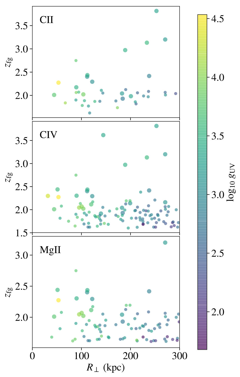 Figure 1
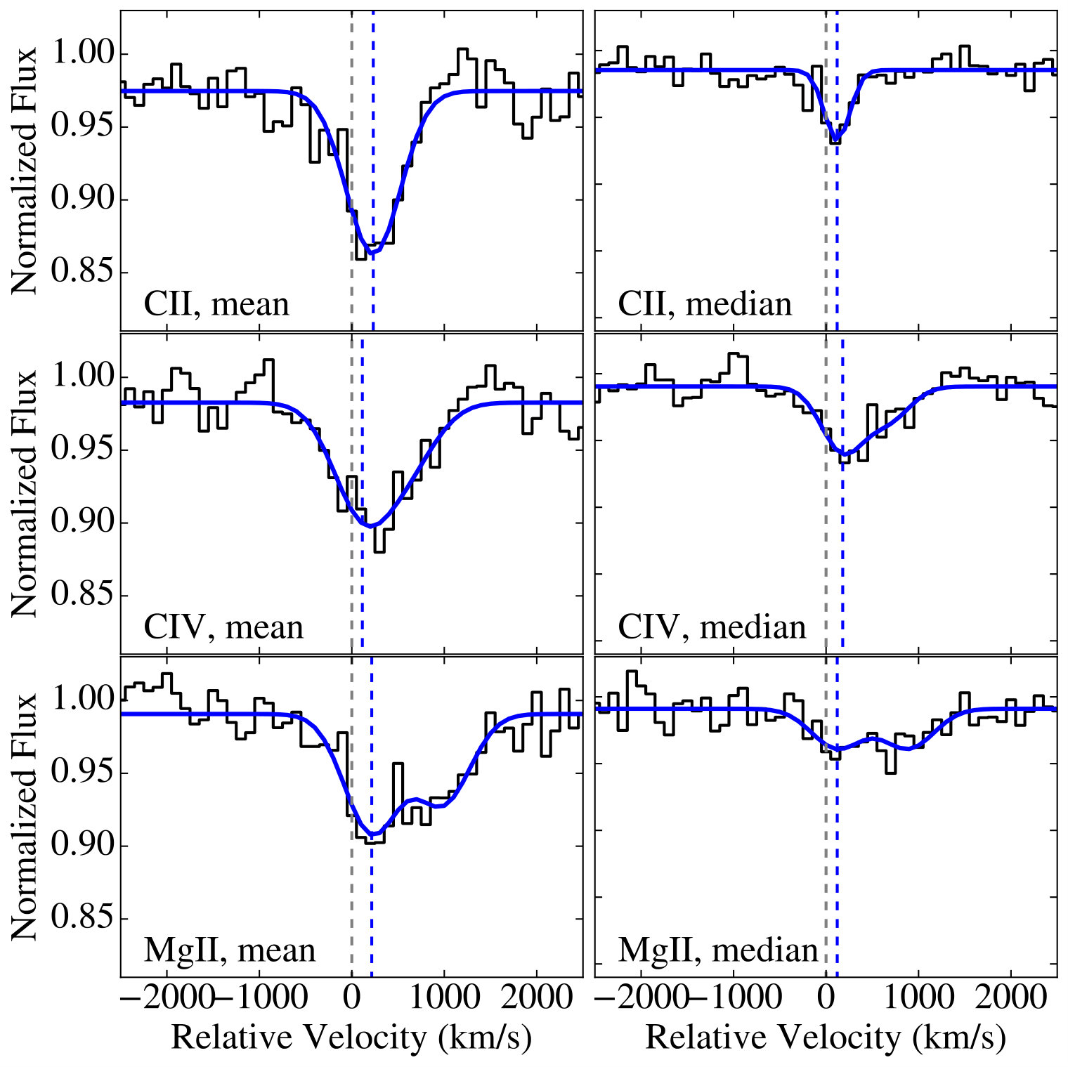 Figure 2
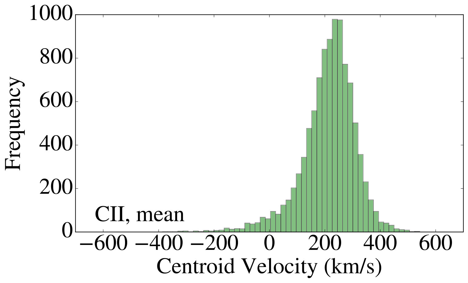 Figure 3
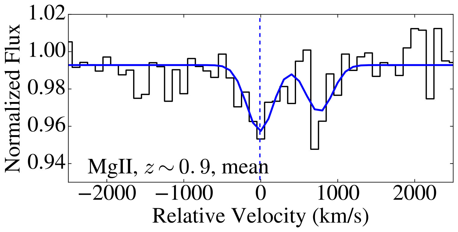 Figure 4
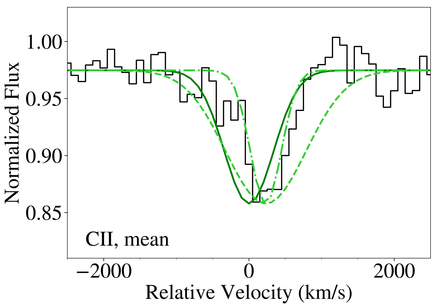 Figure 5
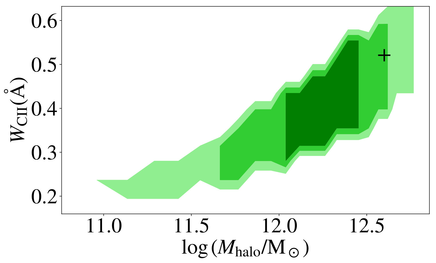 Figure 6
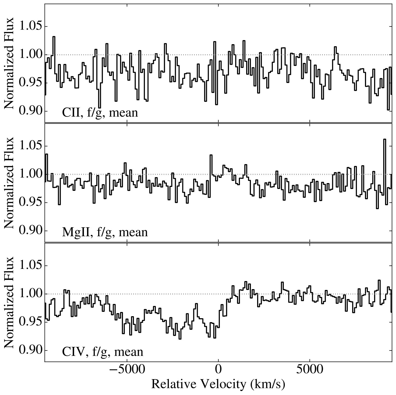 Figure 7
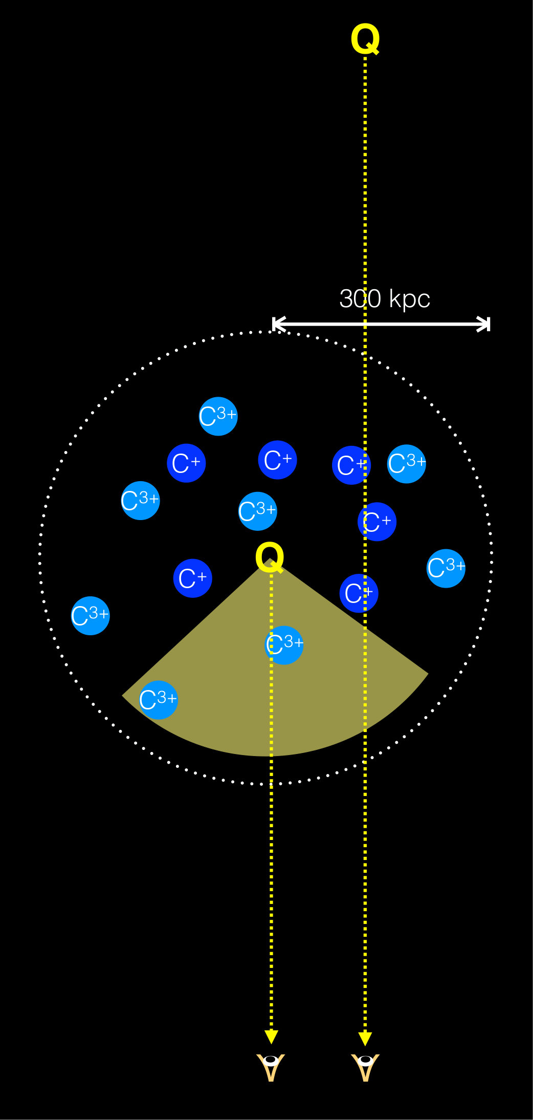 Figure 8
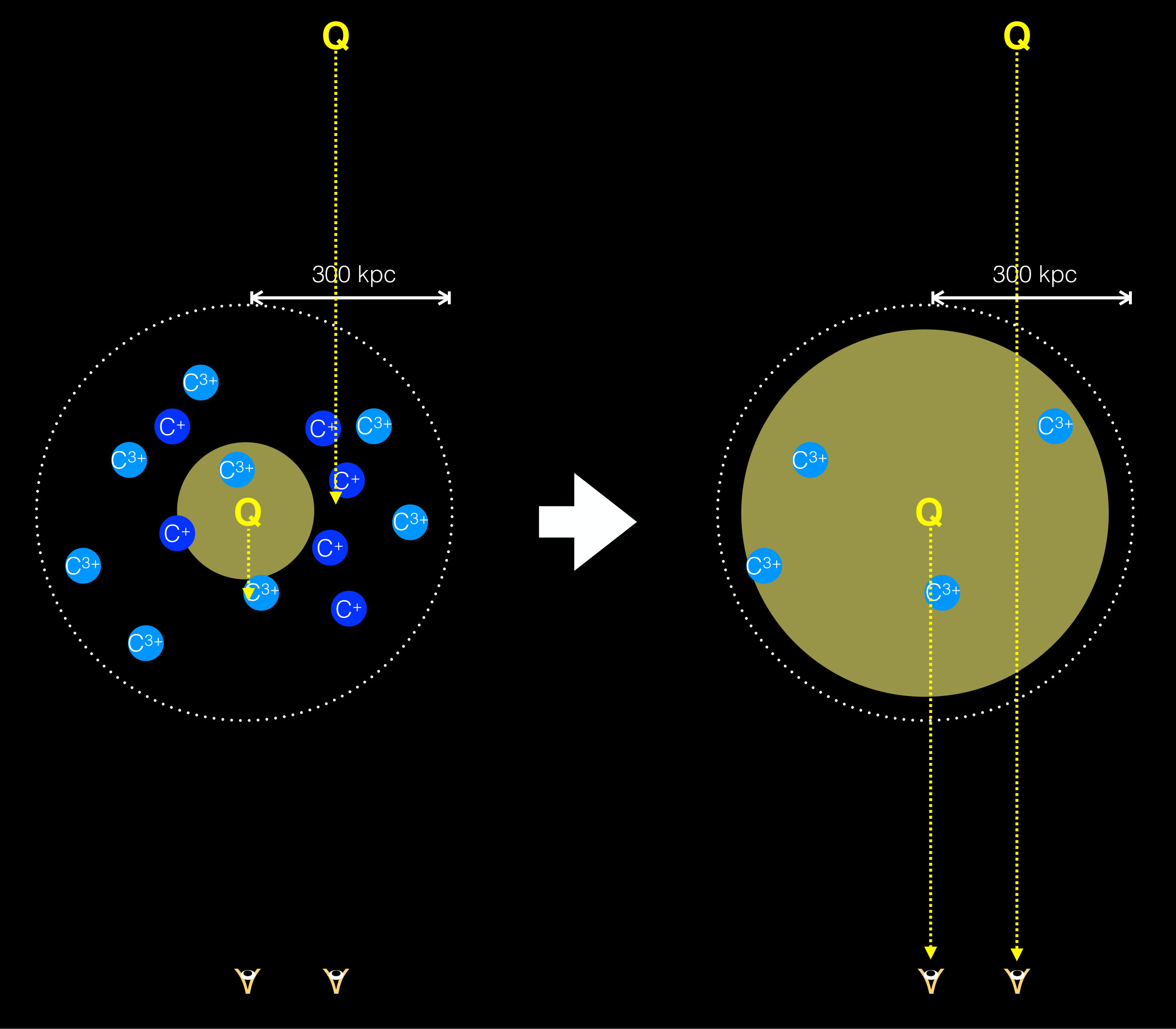 Figure 9
| Foreground Quasar | Line for | Background Quasar | BG Quasar Instrument | (kpc) | |||
|---|---|---|---|---|---|---|---|
| J003423.051050020 | 1.8388 | MgII | J003423.44-104956.3 | 1.948 | LRIS | 67 | 11938 |
| J004220.66+003218.7 | 1.9259 | MgII | J004218.72+003237.1 | 3.048 | BOSS | 299 | 97 |
| J004745.49+310120.3 | 1.9706 | MgII | J004745.61+310138.3 | 2.695 | BOSS | 157 | 1723 |
| J004757.26+144741.0 | 1.6191 | MgII | J004757.88+144744.7 | 2.757 | BOSS | 82 | 6697 |
| J005717.36000113.3 | 2.1611 | [OIII] | J005718.99-000134.7 | 2.511 | BOSS | 271 | 1283 |
| J010323.84000254.2 | 1.7506 | MgII | J010324.37-000251.3 | 2.306 | BOSS | 74 | 5462 |
| J014328.77+295436.8 | 1.8007 | MgII | J014330.89+295439.9 | 2.018 | BOSS | 243 | 997 |
| J014917.11002141.6 | 1.6834 | MgII | J014917.46-002158.5 | 2.159 | SDSS | 155 | 2390 |
| J021416.96005229.1 | 1.8002 | MgII | J021416.12-005251.5 | 2.332 | BOSS | 225 | 564 |
| J022447.89004700.4 | 1.6959 | MgII | J022448.85-004638.9 | 2.188 | BOSS | 226 | 293 |
| J023018.27033319.4 | 2.3817 | MgII | J023019.99-033315.0 | 2.985 | BOSS | 221 | 1444 |
| J023315.44000303.6 | 1.7205 | MgII | J023315.75-000231.4 | 1.839 | BOSS | 286 | 101 |
| J023946.43010640.4 | 2.299 | [OIII] | J023946.45-010644.1 | 3.124 | BOSS | 32 | 20931 |
| J024603.68003211.8 | 1.603 | MgII | J024602.35-003221.6 | 2.153 | BOSS | 195 | 1889 |
| J025038.68004739.2 | 1.8538 | MgII | J025039.82-004749.6 | 2.445 | BOSS | 175 | 4007 |
| J034138.16+000002.9 | 2.1246 | MgII | J034139.19-000012.7 | 2.243 | GMOS-N | 190 | 392 |
| J040955.87041126.9 | 1.7166 | MgII | J040954.21-041137.1 | 2.0 | SDSS | 235 | 715 |
| J072739.55+392855.3 | 1.9853 | MgII | J072739.72+392919.5 | 2.433 | BOSS | 210 | 403 |
| J075009.25+272405.2 | 1.7713 | MgII | J075008.27+272404.5 | 1.802 | LRIS | 114 | 1370 |
| J075259.81+401128.2 | 1.8844 | MgII | J075259.14+401118.2 | 2.121 | SDSS | 110 | 1060 |
| J080049.89+354249.6 | 1.9825 | [OIII] | J080048.74+354231.3 | 2.066 | LRIS | 201 | 2074 |
| J080537.29+472339.3 | 1.8913 | MgII | J080538.78+472404.8 | 2.964 | BOSS | 259 | 367 |
| J080945.17+453918.1 | 2.0392 | MgII | J080948.22+453929.0 | 2.278 | BOSS | 292 | 195 |
| J081223.17+262000.9 | 1.6427 | MgII | J081223.89+262012.5 | 2.17 | BOSS | 132 | 3442 |
| J081419.58+325018.7 | 2.1744 | [OIII] | J081420.38+325016.1 | 2.213 | GMOS-N | 90 | 2899 |
| J081832.87+123219.9 | 1.7032 | MgII | J081833.97+123215.4 | 2.234 | BOSS | 147 | 6609 |
| J082346.05+532527.8 | 1.6467 | MgII | J082347.49+532519.1 | 1.86 | BOSS | 136 | 820 |
| J082421.01+531249.3 | 2.0855 | MgII | J082420.02+531315.2 | 2.165 | BOSS | 237 | 340 |
| J082843.37+454517.3 | 1.873 | MgII | J082844.87+454518.2 | 1.987 | LRIS | 137 | 525 |
| J083030.38+545228.8 | 1.6702 | MgII | J083029.11+545210.3 | 3.337 | BOSS | 188 | 1506 |
| J083713.56+363037.3 | 1.8364 | MgII | J083712.69+363037.7 | 2.301 | MODS1 | 92 | 5012 |
| J083757.91+383727.1 | 2.0624 | H | J083757.13+383722.4 | 2.251 | LRIS | 89 | 8609 |
| J083854.52+462124.4 | 1.7596 | MgII | J083852.94+462137.6 | 2.163 | BOSS | 184 | 673 |
| J084158.47+392120.0 | 2.0414 | [OIII] | J084159.26+392139.0 | 2.214 | LRIS | 183 | 1514 |
| J084511.89+464135.5 | 1.6295 | MgII | J084509.64+464113.0 | 1.898 | BOSS | 283 | 135 |
| J085019.43+475538.5 | 1.8164 | MgII | J085021.17+475516.0 | 1.891 | BOSS | 249 | 392 |
| J085151.38+522901.6 | 1.9738 | MgII | J085154.53+522910.6 | 2.031 | BOSS | 262 | 265 |
| J085249.45+471423.1 | 1.6468 | MgII | J085248.55+471419.3 | 1.688 | BOSS | 87 | 7078 |
| J085358.36001108.0 | 2.4016 | [OIII] | J085357.49-001106.2 | 2.579 | MagE | 112 | 1231 |
| J085629.48+551450.2 | 1.6228 | MgII | J085630.45+551417.5 | 1.932 | BOSS | 296 | 466 |
| J085737.58+390120.5 | 1.9529 | MgII | J085738.00+390136.0 | 2.848 | BOSS | 150 | 1984 |
| J090417.94+004148.2 | 1.6193 | MgII | J090419.12+004205.1 | 1.645 | SDSS | 214 | 1035 |
| J090657.78+100121.4 | 1.6965 | MgII | J090657.62+100105.6 | 2.525 | BOSS | 141 | 6960 |
| J091046.44+041458.5 | 2.0461 | [OIII] | J091046.69+041448.4 | 2.377 | MagE | 95 | 11897 |
| J091217.57+413933.5 | 1.7764 | MgII | J091215.75+413948.2 | 2.198 | BOSS | 220 | 790 |
| J091234.27+305616.2 | 1.6237 | MgII | J091236.32+305626.5 | 2.146 | BOSS | 247 | 514 |
| J091338.33010708.7 | 2.7491 | MgII | J091338.97-010704.6 | 2.916 | XSHOOTER | 89 | 5830 |
| J091432.02+010912.4 | 2.1404 | [OIII] | J091430.85+010927.5 | 2.475 | BOSS | 199 | 1222 |
| J091551.72+011900.2 | 1.9706 | MgII | J091553.37+011911.4 | 2.102 | BOSS | 236 | 970 |
| J092405.06+474611.4 | 2.0556 | MgII | J092402.85+474600.7 | 2.098 | BOSS | 214 | 341 |
| J092417.65+392920.3 | 1.8864 | MgII | J092416.72+392914.6 | 2.08 | LRIS | 106 | 2788 |
| J092543.88+372504.9 | 2.0704 | MgII | J092544.71+372503.5 | 2.314 | BOSS | 94 | 3890 |
| J093226.34+092526.1 | 2.4172 | [OIII] | J093225.66+092500.2 | 2.602 | MagE | 238 | 774 |
| J093317.43+592027.4 | 1.8617 | MgII | J093320.57+592036.5 | 2.633 | BOSS | 224 | 1441 |
| J093640.35005840.1 | 2.2098 | MgII | J093642.12-005831.3 | 2.731 | BOSS | 250 | 496 |
| J093936.83+482115.0 | 1.8878 | MgII | J093938.97+482059.4 | 2.415 | BOSS | 230 | 528 |
| J093952.56+505207.4 | 1.6105 | MgII | J093954.75+505148.8 | 2.476 | BOSS | 242 | 128 |
| J094133.64+230840.1 | 1.7762 | MgII | J094135.61+230845.8 | 2.551 | BOSS | 243 | 1700 |
| J094906.23+465938.4 | 1.7204 | MgII | J094906.52+465909.6 | 2.173 | BOSS | 253 | 243 |
| J095127.06+493248.3 | 1.7407 | MgII | J095126.22+493218.8 | 1.83 | BOSS | 268 | 293 |
| J095858.88+491253.1 | 2.0505 | MgII | J095858.06+491307.5 | 2.155 | BOSS | 144 | 722 |
| J100046.45+033708.8 | 1.7006 | MgII | J100048.52+033708.8 | 2.353 | BOSS | 271 | 255 |
| J100509.56+501929.8 | 1.8176 | MgII | J100507.07+501929.8 | 2.019 | LRIS | 211 | 330 |
| J100627.47+480420.0 | 2.3034 | [OIII] | J100627.11+480429.9 | 2.597 | BOSS | 90 | 2886 |
| J100913.91+023612.4 | 1.7359 | MgII | J100913.33+023643.0 | 2.216 | BOSS | 287 | 342 |
| J100941.35+250104.1 | 1.8703 | MgII | J100940.58+250053.9 | 1.981 | LRIS | 127 | 3588 |
| J101001.51+403755.5 | 2.1924 | H | J101003.47+403754.9 | 2.505 | BOSS | 191 | 5421 |
| J101323.89+033016.0 | 1.9401 | MgII | J101322.23+033009.1 | 2.273 | BOSS | 219 | 426 |
| J101753.38+622653.4 | 1.6528 | MgII | J101750.44+622648.2 | 2.738 | BOSS | 184 | 922 |
| J101947.11+494835.8 | 1.6224 | MgII | J1019470+494849.1 | 1.652 | LRIS | 117 | 881 |
| J102007.23+611955.0 | 1.7909 | MgII | J102010.05+611950.3 | 2.387 | BOSS | 180 | 1817 |
| J102259.33+491125.8 | 1.9757 | MgII | J102259.97+491151.7 | 2.469 | BOSS | 231 | 212 |
| J102821.26+240121.8 | 1.8709 | MgII | J102822.18+240057.4 | 2.414 | BOSS | 240 | 834 |
| J103443.62+085702.0 | 1.6395 | MgII | J103442.26+085645.7 | 2.766 | BOSS | 233 | 700 |
| J103628.12+501157.9 | 2.0097 | MgII | J103630.52+501219.8 | 2.228 | BOSS | 271 | 1198 |
| J103857.37+502707.0 | 3.1325 | [OIII] | J103900.01+502652.8 | 3.236 | ESI | 233 | 3567 |
| J103946.92+454716.0 | 1.8644 | MgII | J103945.58+454707.4 | 2.456 | BOSS | 148 | 675 |
| J104244.84+650002.7 | 1.9876 | MgII | J104245.14+645936.7 | 2.124 | BOSS | 227 | 703 |
| J104435.62+313950.7 | 1.7062 | MgII | J104434.76+313957.7 | 2.377 | BOSS | 115 | 1873 |
| J104955.01+231358.2 | 1.8439 | MgII | J104953.97+231401.3 | 2.171 | BOSS | 129 | 1813 |
| J105221.77+555253.5 | 1.9989 | MgII | J105218.36+555311.3 | 2.278 | BOSS | 293 | 846 |
| J105246.45+641832.2 | 1.6429 | MgII | J105251.42+641838.5 | 2.936 | BOSS | 286 | 127 |
| J111339.86+330604.8 | 1.8913 | MgII | J111337.84+330553.3 | 2.413 | BOSS | 243 | 853 |
| J111850.44+402553.8 | 1.9257 | MgII | J111851.45+402557.6 | 2.317 | BOSS | 106 | 1946 |
| J112858.89+644440.4 | 1.6561 | MgII | J112854.14+644427.4 | 2.217 | BOSS | 289 | 149 |
| J113852.65+632934.0 | 1.8855 | MgII | J113851.73+632955.6 | 2.625 | BOSS | 196 | 1912 |
| J114435.54+095921.7 | 2.9734 | [OIII] | J114436.65+095904.9 | 3.16 | MIKE-Red | 189 | 2914 |
| J114439.51+454115.8 | 1.687 | MgII | J114442.48+454111.3 | 2.592 | BOSS | 275 | 78 |
| J114546.54+032236.7 | 1.7664 | MgII | J114546.22+032251.9 | 2.011 | MagE | 139 | 779 |
| J115253.09+150706.5 | 1.7883 | MgII | J115254.97+150707.8 | 3.349 | BOSS | 237 | 622 |
| J115457.16+471149.3 | 1.6819 | MgII | J115458.69+471209.9 | 1.947 | SDSS | 226 | 60 |
| J115502.45+213235.5 | 1.9551 | MgII | J115504.25+213254.0 | 2.695 | BOSS | 277 | 397 |
| J115529.49+463413.1 | 1.6491 | MgII | J115528.75+463442.9 | 2.329 | BOSS | 270 | 326 |
| J115533.62+393359.2 | 1.6118 | MgII | J115531.32+393415.4 | 2.555 | BOSS | 272 | 742 |
| J120224.68+074800.3 | 1.6613 | MgII | J120226.48+074739.7 | 2.767 | BOSS | 296 | 584 |
| J120417.47+022104.7 | 2.436 | [OIII] | J120416.69+022110.0 | 2.532 | HIRES | 112 | 2710 |
| J120856.94+073741.2 | 2.1708 | MgII | J120857.16+073727.3 | 2.616 | MagE | 123 | 3853 |
| J121159.88+324009.0 | 1.978 | MgII | J121201.69+324013.3 | 2.273 | BOSS | 209 | 1046 |
| J121344.28+471958.7 | 1.8371 | MgII | J121343.01+471931.0 | 3.275 | BOSS | 260 | 491 |
| J1215590+571616.6 | 1.93 | [OIII] | J121558.82+571555.5 | 1.964 | BOSS | 184 | 614 |
| J121657.82+152706.6 | 1.9473 | MgII | J121657.00+152712.7 | 2.318 | BOSS | 116 | 4225 |
| J122514.29+570942.3 | 1.8953 | MgII | J122517.89+570943.7 | 2.224 | BOSS | 255 | 330 |
| J123143.01+002846.3 | 3.2015 | [OIII] | J123141.73+002913.9 | 3.308 | GMOS-S | 271 | 1490 |
| J124632.33+234531.2 | 1.9937 | MgII | J124632.19+234509.5 | 2.573 | BOSS | 188 | 1886 |
| J124846.05+405758.2 | 1.8265 | MgII | J124846.97+405820.9 | 2.463 | BOSS | 219 | 897 |
| J130124.74+475909.6 | 2.194 | H | J130125.67+475930.8 | 2.765 | SDSS | 199 | 4932 |
| J130605.19+615823.7 | 2.1089 | H | J130603.55+615835.2 | 2.175 | LRIS | 141 | 1761 |
| J130714.79+463536.6 | 1.6226 | MgII | J130716.07+463511.2 | 2.248 | BOSS | 251 | 137 |
| J131341.32+454654.6 | 1.6878 | MgII | J131342.78+454658.2 | 2.241 | BOSS | 139 | 1098 |
| J132514.97+540930.6 | 2.0507 | MgII | J132511.07+540927.0 | 3.235 | BOSS | 298 | 514 |
| J133026.12+411432.0 | 2.0645 | MgII | J133023.67+411445.9 | 2.217 | BOSS | 271 | 384 |
| J133924.02+462808.2 | 1.8539 | MgII | J133922.31+462749.2 | 3.391 | BOSS | 226 | 940 |
| J134650.08+195235.2 | 2.0697 | MgII | J134648.19+195253.1 | 2.523 | BOSS | 278 | 884 |
| J135306.35+113804.7 | 1.6315 | MgII | J135307.90+113805.5 | 2.431 | BOSS | 213 | 8963 |
| J135849.71+273806.9 | 1.9008 | MgII | J135849.54+273756.9 | 2.127 | LRIS | 89 | 1765 |
| J140208.01+470111.1 | 1.9161 | [OIII] | J140209.52+470117.8 | 2.269 | BOSS | 140 | 1437 |
| J140918.01+522552.4 | 1.8808 | MgII | J140916.98+522535.3 | 2.109 | SDSS | 170 | 583 |
| J141337.18+271517.1 | 1.6905 | MgII | J141337.96+271511.0 | 1.965 | BOSS | 105 | 609 |
| J142003.67+022726.7 | 3.617 | [OIII] | J142004.12+022708.8 | 4.191 | ESI | 144 | 2291 |
| J142054.42+160333.3 | 2.0221 | [OIII] | J142054.92+160342.9 | 2.057 | MagE | 104 | 7811 |
| J142215.57+465230.7 | 1.748 | MgII | J142214.63+465254.6 | 2.338 | BOSS | 225 | 639 |
| J142758.89012130.4 | 2.2738 | [OIII] | J142758.74-012136.2 | 2.354 | MIKE | 53 | 34208 |
| J143109.67+572728.0 | 1.6802 | MgII | J143109.22+572726.4 | 2.063 | BOSS | 39 | 5166 |
| J143312.56+082651.8 | 1.8807 | MgII | J143313.99+082714.0 | 2.432 | BOSS | 274 | 531 |
| J143345.55+064109.0 | 2.294 | [OIII] | J143344.55+064111.9 | 2.34 | BOSS | 122 | 1130 |
| J143609.15+313426.7 | 1.8774 | MgII | J143610.68+313418.9 | 2.562 | BOSS | 183 | 2188 |
| J144211.25+530252.0 | 1.6461 | MgII | J144209.98+530308.0 | 2.632 | BOSS | 179 | 439 |
| J144232.92+013730.4 | 1.8079 | MgII | J144231.91+013734.8 | 2.274 | BOSS | 137 | 1988 |
| J144429.34+311321.2 | 1.7355 | MgII | J144427.96+311313.0 | 1.795 | LRIS | 173 | 8820 |
| J150814.06+363529.4 | 1.8493 | MgII | J150812.78+363530.3 | 2.105 | BOSS | 133 | 5111 |
| J153328.83+142542.5 | 2.0782 | MgII | J153329.17+142537.8 | 2.564 | BOSS | 59 | 3898 |
| J153456.02+215342.3 | 1.6712 | MgII | J153455.85+215324.7 | 2.529 | BOSS | 156 | 1702 |
| J153954.74+314629.3 | 1.8747 | MgII | J153952.46+314625.2 | 2.235 | BOSS | 256 | 1080 |
| J155325.61+192140.0 | 2.01 | [OIII] | J155325.89+192137.7 | 2.098 | MagE | 44 | 5576 |
| J155422.88+124438.0 | 1.8169 | MgII | J155424.39+124431.5 | 2.394 | BOSS | 202 | 1349 |
| J155947.73+494307.3 | 1.8615 | MgII | J155946.28+494326.7 | 1.945 | LRIS | 210 | 1743 |
| J160547.61+511330.5 | 1.783 | MgII | J160546.67+511322.9 | 1.844 | LRIS | 102 | 4045 |
| J161930.94+192620.9 | 1.7821 | MgII | J161929.78+192645.4 | 2.39 | BOSS | 258 | 538 |
| J162738.63+460538.4 | 3.8149 | [OIII] | J162737.25+460609.3 | 4.11 | ESI | 253 | 1959 |
| J163121.74+433317.3 | 2.0182 | MgII | J163123.57+433317.3 | 2.631 | BOSS | 172 | 4090 |
| J165442.21+251249.2 | 1.7207 | MgII | J165444.38+251306.2 | 2.341 | BOSS | 298 | 459 |
| J165716.85+310513.0 | 2.1331 | MgII | J165716.52+310524.5 | 2.395 | MODS1 | 98 | 5222 |
| J214620.69075250.6 | 2.1155 | [OIII] | J214620.99-075303.8 | 2.577 | MagE | 120 | 4869 |
| J214813.26+263059.4 | 1.6285 | MgII | J214814.36+263129.7 | 3.286 | BOSS | 295 | 78 |
| J220248.61+123645.5 | 2.0697 | [OIII] | J220248.31+123656.3 | 2.512 | BOSS | 100 | 9466 |
| J233845.19000327.1 | 2.4399 | [OIII] | J233845.45-000331.8 | 2.997 | XSHOOTER | 51 | 3674 |
| J235505.22+320058.0 | 1.8159 | MgII | J235505.33+320105.4 | 2.367 | BOSS | 56 | 2271 |
| J235819.92+342455.8 | 1.6235 | MgII | J235819.33+342506.5 | 2.02 | BOSS | 113 | 480 |
| Measure | C II 1334 | C IV 1548 | Mg II 2796 |
|---|---|---|---|
| For the Full QPQ9 Sample | |||
| Number of pairs | 40 | 110 | 86 |
| Median | 2.04 | 1.89 | 1.87 |
| Median | 157 | 191 | 184 |
| 1 dispersion of mean stack () | |||
| Centroid of mean stack () | |||
| Pseudo-continuum of mean stack | |||
| 1 dispersion of median stack () | |||
| Centroid of median stack () | |||
| Pseudo-continuum of median stack | |||
| For the Sub-sample with [OIII] Redshifts | |||
| Number of pairs | 15 | 23 | 15 |
| Median | 2.29 | 2.29 | 2.27 |
| Median | 183 | 122 | 112 |
| 1 dispersion of mean stack () | |||
| Centroid of mean stack () | |||
| Pseudo-continuum of mean stack | |||
| 1 dispersion of median stack () | |||
| Centroid of median stack () | |||
| Pseudo-continuum of median stack | |||
Peer Reviews
No public reviews on file for this paper yet. If you reviewed it on a platform where reviews are public (OpenReview, ICLR, NeurIPS, ICML), you can paste yours below so the community can read it here.
Videos
No videos yet. Explain this paper in a talk, walkthrough, or lecture? Add one.
Quasars Probing Quasars IX. The Kinematics of the Circumgalactic Medium Surrounding
Quasars
Marie Wingyee Lau11affiliation: Email: [email protected] 22affiliation: Department of Astronomy and Astrophysics, UCO/Lick Observatory, University of California, 1156 High Street, Santa Cruz, CA 95064 , J. Xavier Prochaska22affiliation: Department of Astronomy and Astrophysics, UCO/Lick Observatory, University of California, 1156 High Street, Santa Cruz, CA 95064 , Joseph F. Hennawi33affiliation: Department of Physics, Broida Hall, University of California, Santa Barbara, CA 93106-9530
Abstract
We examine the kinematics of the gas in the environments of galaxies hosting quasars at . We employ 148 projected quasar pairs to study the circumgalactic gas of the foreground quasars in absorption. The sample selects foreground quasars with precise redshift measurements, using emission-lines with precision and average offsets from the systemic redshift . We stack the background quasar spectra at the foreground quasar’s systemic redshift to study the mean absorption in C II, C IV, and Mg II. We find that the mean absorptions exhibit large velocity widths . Further, the mean absorptions appear to be asymmetric about the systemic redshifts. The mean absorption centroids exhibit small redshift relative to the systemic , with large intrinsic scatter in the centroid velocities of the individual absorption systems. We find the observed widths are consistent with gas in gravitational motion and Hubble flow. However, while the observation of large widths alone does not require galactic-scale outflows, the observed offsets suggest that the gas is on average outflowing from the galaxy. The observed offsets also suggest that the ionizing radiation from the foreground quasars is anisotropic and/or intermittent.
Subject headings:
galaxies: clusters: intracluster medium – galaxies: formation – galaxies: halos – intergalactic medium – quasars: absorption lines – quasars: general
1. Introduction
Galaxy formation and evolution are driven by the flows of gas into and out of their interstellar medium. Current theories demand that star-forming galaxies maintain these flows. Gas accretes, cools, and adds to the fuel supply, while star formation feedback heats gas, blows it out of galaxies, and regulates star formation (for a review see Somerville & Davé, 2015).
Direct observations of galactic flows are difficult to acquire. Detecting the presence of the gas is itself challenging. Either the gas mass is too small, or the gas density is too low for the detection of line-emission, e.g. 21 cm, Ly, or H from H I. Resolving the kinematics and establishing the mass flux pose an even greater challenge. These challenges are accentuated for distant, young galaxies, where flows of gas are predicted to prevail (Kereš et al., 2009; Fumagalli et al., 2011). Therefore, with rare exceptions, (e.g., Cantalupo et al., 2014; Hennawi et al., 2015), the community has relied on absorption-line spectroscopy to detect and characterize the gas surrounding galaxies (e.g., Bergeron & Boisse, 1991; Steidel et al., 2010; Prochaska et al., 2011; Tumlinson et al., 2013). In a previous paper of the Qussars Probing Quasars series (Lau et al., 2016, , hereafter QPQ8), we measured the velocity field for C II 1334 and C IV 1548, finding that the circumgalactic medium frequently exhibits large velocity widths that are offset from the systemic redshift. From a sample of 7 C II systems and 10 C IV systems, we measured the velocity interval that encompasses 90% of the total optical depth, , and the dispersion relative to the profile centroid, . The median is for C II 1334 and is for C IV 1548. The median is for C II 1334 and is for C IV 1548. These velocity fields exceed all previous measurements from galaxies and/or absorption systems at any epoch. The offsets, , are often positive, with the sign convention that positive velocities indicate a redshift from the systemic.
With absorption-line spectroscopy of background sightlines, other researchers also have had success in characterizing the flows of gas around galaxies. Rakic et al. (2012) found a net large-scale inflow around star-forming galaxies, or a Kaiser effect for gas on 1–2 Mpc scales. Ho et al. (2017) found gas spiraling inward near the disk plane of star-forming galaxies on kpc scales. Johnson et al. (2015) studied the CGM surrounding quasars. They found large peculiar motions in the gas exceeding the expected virial velocity, with quasar-driven outflows being one possible explanation. However, we consider that their velocity spreads can be better quantified. Other existing studies that found large velocity spreads are single sightlines (e.g., Tripp et al., 2011; Rudie et al., 2017), or with gas tracing a higher ionization state than the QPQ absorption systems (e.g., Churchill et al., 2012), or where the average velocity spread is smaller than that measured in QPQ8. In Gauthier (2013), where a single sightline is reported, the of the Mg II absorption is less than the average of the QPQ8 C II absorption. In Muzahid et al. (2015), an absorber is found with smaller than in O VI and N V, and still smaller for other ions. The Zahedy et al. (2016) sample likewise has average smaller than that of QPQ8.
A significant limitation of absorption-line analysis of transverse sightlines, especially regarding galactic-scale flows, is the inherent symmetry of the experiment. One generally lacks any constraint on the distance of the gas along the sightline. Positive or negative velocities with respect to the galaxy may be interpreted as gas flowing either toward or away from the system. “Down-the-barrel” observations break this symmetry, and have generally provided evidence for flows away from galaxies (Rupke et al., 2005; Martin, 2005; Weiner et al., 2009; Rubin et al., 2014). However, these data are frequently at low spectral resolution which limits one’s sensitivity to inflowing gas.
In this paper (hereafter QPQ9), we examine the flows of gas in the environments of massive galaxies hosting quasars. Our approach leverages a large dataset of quasar pairs (Hennawi et al., 2006, hereafter QPQ1) to use the standard techniques of absorption-line spectroscopy with background quasars. These quasar pairs have angular separations that correspond to less than 300 kpc projected separation at the foreground quasar’s redshift. Our previous publications from these quasar pairs have established that these galaxies are surrounded by a massive, cool, and enriched CGM (QPQ5, QPQ6, QPQ7: Prochaska et al., 2013b, a, 2014). We have collected a sample of 148 background spectra that are paired with foreground quasars with precisely measured redshifts. Among the sightlines in the QPQ9 sample, 13 have spectral resolution from echellette or echelle observations, and have been analyzed separately in QPQ8 (see their Figure 8, 9, and 10, and their Appendix). In QPQ8, where the individual metal-bearing absorption components are resolved, 15 out of the 21 components are at positive velocities relative to the systemic redshift. For this current work, we stack spectra of all resolutions instead of performing a component-by-component analysis. Our primary scientific interests are twofold: (i) search for signatures of galactic-scale outflows from the central galaxy, presumably driven by recent star formation and/or active galactic nuclei feedback; (ii) characterize the dynamics of the gas around these massive systems. We further describe an aspect of this experiment that offers a unique opportunity to study galactic-scale flows: we argue that, the anisotropic or intermittent radiation from the foreground quasars may break the symmetry in the velocity field of circumgalactic absorbers. If the ionizing radiation field is asymmetric, the absorbers may also distribute asymmetrically. Alternatively, finite quasar lifetime will result in different radiation fields impinged on the gas closer to versus further away from the background quasar, due to different light travel times. Kirkman & Tytler (2008) reported an asymmetry in H I absorption on scales larger than the CGM, and gave similar arguments on anisotropy or intermittence.
We adopt a CDM cosmology with , and . Distances are proper unless otherwise stated. When referring to comoving distances we include explicitly an term and follow modern convention of scaling to the Hubble constant .
2. The Experiment
The goal of our experiment is to measure the average velocity fields of the absorption from C+, C3+, and Mg+ ions associated with the CGM of the galaxies hosting quasars.
From our QPQ survey111http://www.qpqsurvey.org, we analyze a subset of systems that pass within transverse separation kpc from a foreground quasar with . We restrict the sample to foreground quasars with redshift measured from Mg II 2800, [O III] 5007, or H emission, giving a precision of or better and an average offset from the systemic redshift of or less. According to Shen et al. (2016a), the [O III] emission-line redshifts have the smallest scatter (intrinsic scatter and measurement error combined) of about the systemic redshift, and we analyze the sub-sample with [O III] redshifts separately. The [O III] line has an average blueshift of about the systemic redshift, which has been added when we compute the redshift of the line. The scatter and average offset of [O III] redshifts reported by Shen et al. (2016a) is consistent with the numbers reported by Boroson (2005) using a larger but lower redshift sample. Systemic redshifts measured from Mg II have a precision of according to Shen et al. (2016a), and we have taken into account their reported median blueshift of of Mg II from the systemic. We note that Richards et al. (2002) reported a median redshift of of Mg II from [O III] using a larger but lower redshift sample. In QPQ8, we quantified the precision of H to be and the median offset from the systemic redshift is close to zero, consistent with the velocity shifts measured by Shen et al. (2011). Although H is a narrow emission-line, we do not consider its redshift sufficiently reliable for use as systemic redshift. H redshifts have a large scatter about the systemic , and a large average offset about the systemic (Shen et al., 2016a, QPQ8). Our line-centering algorithm calculates the mode of a line given by , applied to the upper 60% of the emission, while Shen et al. (2016a) calculates the peak of a line. We expect that our line-centering algorithm gives emission redshifts very comparable to the Shen et al. (2016a) algorithm, however. Shen et al. (2016a) states that the difference between the peak and the centroid of an emission-line is not significant except for the broad line H, which we do not use in redshift measurements. To quantify the above, we further obtain individual measurements of centroids and peaks in the Shen et al. (2016a) sample through private communication. We found there is essentially no difference between using the centroid versus using the peak for [O III] emission redshifts, and there is on average difference for Mg II. We may expect the difference between the mode and the peak is even smaller. Hence, we argue that the average systemic bias corrections measured in Shen et al. (2016a) may be self-consistently applied to our measured emission-line redshifts to obtain systemic redshifts.
We further add to the QPQ dataset with quasar pairs selected from the public dataset of igmspec222https://github.com/specdb/igmspec (Prochaska, 2017), which includes the spectra from the quasar catalogs based upon the Sloan Digital Sky Survey Seventh Data Release (Schneider et al., 2010) and the Twelfth Data Release (Pâris et al., 2017). We only select pairs with measurable using a robust Mg II 2800 emission-line. We reach a final sample size of 148. Figure 1 summarizes the experimental design. We refer the reader to previous QPQ publications for the details on the emission-line centering algorithm, data reduction, and continuum normalization (QPQ1; QPQ6; QPQ8).
As in the previous QPQ papers, we select the quasar pairs to have redshift difference , to exclude physically associated binary quasars. The cut on velocity difference is motivated by the typical redshift uncertainty of of the background quasars. In QPQ8, it was required that the observed wavelengths of the metal ion transitions fall outside the Ly forest of the background quasar. In this paper, we exclude a small window around the Ly emission, in additional to the Ly forest, from analysis. For stacked profile analysis, a good estimate of the continuum level is necessary. In QPQ8 we found that absorption associated to the foreground quasar occurs within around . Therefore, it is desirable to keep a window relatively free of contamination from Ly forest. Taking into account the redshift uncertainties, we decide that at least one transition among C II 1334, C IV 1548, and Mg II 2796 at must lie redward of , for a pair to be included in the analysis.
Furthermore, we include only those spectra with average signal-to-noise ratio (S/N) exceeding 5.5 per rest-frame Å in a window centered on the observed wavelengths of the metal ion transitions. This criterion is a compromise between maximizing sample size versus maintaining good data quality on the individual sightlines. We find that S/N per rest-frame Å is necessary for properly estimating the continuum, as well as identifying mini-broad absorption line systems associated to the background quasar, which will significantly depress the flux level. We also require that the region of the spectrum that is around a considered metal ion transition does not overlap with strong atmospheric bands. The A- and B-band span 7595–7680 Å and 6868–6926 Å respectively.
Table 1 lists the full QPQ9 sample. In Table 2, we first list the sample size, the median , and the median of the quasar pairs that survive the above selection criteria for C II 1334, C IV 1548, and Mg II 2796 respectively. We then provide the summary for the sub-sample with measured from [O III].
3. Analysis
3.1. Stacked Profiles
We create composite spectra that average over the intrinsic scatter in quasar environments, continuum placement errors, and redshift errors. The individual spectra of background quasars are shifted to the rest-frame of the foreground quasars at the transitions of interest. Each spectrum has been linearly interpolated onto a fixed velocity grid centered at with bins of . For a velocity bin of this size, it is unnecessary to smooth the data to a common spectral resolution. The individual spectra are then combined with a mean or a median statistic. Spectra with broad absorption-line systems and mini-broad absorption-line systems are excluded. Bad pixels in the individual spectra have been masked before generating the composites. Since each quasar pair gives an independent probe of the CGM, each pair has an equal weighting in the stacked profiles, i.e. we do not weight the spectra by the measured S/N near the metal ion transitions. Scatter in the stacked spectra is dominated by randomness in the CGM rather than scatter in the flux of individual observations. The mean statistic of the individual spectra yields a good estimate of the average absorption and preserves equivalent width. The median statistic is less sensitive to outliers. However, the median opacity at any velocity channel is rather small, since the discrete absorbers are spread throughout the entire velocity window. A pixel is not affected unless there are more than 50% of quasar pairs with absorption at its velocity. The analysis on the median velocity field is thus subject to larger uncertainty. In the following we present stacked spectra using both the mean and the median statistic.
In Figure 2, we present mean and median stacks of C II 1334, C IV 1548, and Mg II 2796 absorption of the QPQ9 sample. We focus on the analysis results of the C II mean stack. C IV and Mg II are doublet transitions and it is more challenging to analyze their kinematics. Two results are evident in Figure 2: (i) the mean C II stack exhibits excess absorption spanning a large velocity width; (ii) the mean absorption is likely skewed toward positive velocities.
Visually, there are two absorption components. One component is the uniform depression in the continuum level in the stack resulting from absorbers unassociated with the foreground quasars. The other component comes from absorbers associated with the foreground quasars and distribute around their systemic velocities. To model the absorption, we introduce a Gaussian profile while allowing a constant “pseudo-continuum” to vary. We perform minimization with each channel given equal weight. From the best-fit to the data, we measure the dispersion of the stack to be and the centroid of the C II stack to be . The dispersion suggests extreme kinematics, while the centroid suggests an asymmetry that contradicts the standard expectation. The median stack, on the other hand, shows weaker absorption, and the Gaussian model has a more uncertain dispersion and a centroid with smaller offset.
To test whether the dispersion in the average absorption associated with the foreground quasars is well-captured by a Gaussian model, we also calculate the dispersion separately using the standard deviation formula. Specifically, we apply the standard deviation formula to a window surrounding the absorption centroid, while fitting a continuum to the rest of the window for stacking. The dispersion measured with the above method is essentially the same as that found by fitting a Gaussian. One may also speculate on the existence of a broader absorption component hidden in the depressed continuum. We try replacing the constant absorption component with a broad Gaussian component in our modeling. We find that this second Gaussian component has an amplitude of , i.e. essentially the same amplitude as the initial constant absorption component, and a dispersion of , i.e. wider than the entire velocity window for stacking. This weak and very broad component has no effect on the width and the centroid of the narrow, associated Gaussian component. We therefore consider that one single Gaussian component is a good description of the average absorption associated with the foreground quasars. Moreover, narrow associated absorbers of background quasars will not prefer the systemic velocities of the foreground quasars, and hence will not affect the average absorption measured for the foreground quasars. Their contribution to the average absorption should result in a tilt in the pseudo-continuum, which is insignificant.
We also create mean and median stack for the sub-sample with [O III] redshifts and model the absorption with Gaussian best-fit. The C II mean stack for this sub-sample has a dispersion of , and a centroid at , consistent with the full sample.
To model the mean and median absorption of C IV 1548 and Mg II 1796, we introduce a second Gaussian with separation equal to the doublet separation ( and respectively), and tie the dispersion of the two lines in a doublet. We allow the doublet ratio to vary from 2:1 to 1:1. The centroid is degenerate with the doublet ratio in our modeling. This degeneracy is more pronounced for C IV, although we find that a double ratio closer to 2:1 better captures the absorption at the central few pixels. We state that the modeling of the doublets is presented for consistency check, but the analysis focuses on C II. The modeling results show that the velocity fields of C IV and Mg II are consistent with C II, i.e. large dispersion and centroid is skewed toward positive velocities.
The above analyses are summarized in Table 2. The Gaussian models normalized to pseudo-continuum are overplotted on the data stacks in Figure 2.
3.2. Interpretation of the large velocity fields
Under the assumption that the intrinsic dispersion and the redshift uncertainty add in quadrature to give the observed width, we solve for the intrinsic dispersion in the C II mean stack. For the full QPQ9 sample, with the mean , we recover . For the sub-sample with [O III] redshifts, we recover .
To assess the statistical significance of the observed dispersion, we perform a bootstrap analysis by randomly resampling from the full sample 10000 times. We introduce a Gaussian absorption profile to model each bootstrap realization. We find that a width of would be larger than the observed by three times the scatter in the bootstrap realizations (overplotted in Figure 3). In other words, taking into account the redshift errors, motions in addition to gravitational and Hubble flows that will produce an intrinsic dispersion can be ruled out.
On the contrary, together with Hubble velocities and broadening by redshift errors will result in a velocity width that is more than three times the modeling error away from the observed width (overplotted in Figure 3). This implies that, unless the characteristic , additional dynamical processes are not required to explain the observed width.
Eftekharzadeh et al. (2015) measured the clustering of quasars in the range while Rodríguez-Torres et al. (2017) measured the clustering of quasars in the range . They estimated that these quasars are hosted by dark matter halos with mass and respectively. If dark matter halos hosting QPQ9 quasars have a characteristic mass and follow an NFW profile (Navarro et al., 1997) with concentration parameter , at the maximum circular velocity is . Tormen et al. (1997) found that the maximum circular velocity is times the maximum of the average one-dimensional root-mean-square velocity . Hence, the average line-of-sight rms velocity typical of QPQ9 halos is . In QPQ8, we estimated the probability of intercepting a random optically thick absorber is 4%, and clustering would only increase that to 24%. Although motions due to Hubble flows do not dominate, they nevertheless contribute to the observed dispersion. We can investigate whether gravitational motions and Hubble flows are sufficient to reproduce the dispersion in the data, using Monte Carlo methods to simulate the absorption signals.
Since C II systems arise in optically thick absorbers, we may adopt the clustering analysis results of QPQ6. In the absence of clustering, the expected number of absorbers per unit redshift interval for Lyman limit systems, super Lyman limit systems, and damped Ly systems are respectively , , and . The quasar-absorber correlation functions for Lyman limit systems, super Lyman limit systems, and damped Ly systems are respectively , , and . For each quasar pair, we calculate the expected number of optically thick absorbers within at a distance from the foreground quasar and at . Then we generate 1000 mock sightlines. The number of absorbers for each mock spectrum is randomly selected from a Poisson distribution with mean equal to the expected number calculated as above. The absorbers are randomly assigned Hubble velocities, with a probability distribution according to the quasar-absorber correlation functions. The absorbers are randomly assigned additional peculiar velocities drawn from a normal distribution with mean equal to and scatter equal to . For each absorber, we assume a rest equivalent width for C II and a Gaussian absorption profile. We repeat the above procedure for all 40 quasar pairs, and create a mean stack of the 40000 mock spectra generated. We fit a Gaussian absorption profile multiplied to a constant continuum level to model the stack of mock spectra. We adjust the adopted for the absorbers until the amplitude of the best-fit Gaussian of the stack of mock spectra matches the amplitude of the stack of the observational data. We find that well reproduces the amplitude, and the dispersion of the Gaussian absorption model is insensitive to the assumed or line profile for one absorber.
In Figure 3, we show a comparison of the observational data stack and the Gaussian absorption model of the Monte Carlo simulations. n the figure, the Gaussian absorption model is broadened by the mean redshift error by adding it in quadrature to the dispersion in the model. The resulting stack of mock spectra has a dispersion of , about 2 times the modeling error away from the intrinsic dispersion in the C II mean stack for the full sample, and about 2 times the modeling error away from the intrinsic dispersion in the stack of the sub-sample with [O III] redshifts as well. One may also consider whether absorbers in Hubble flow and cosmological distances show peculiar velocities that are typical for quasar-mass halos, and adopt a different accordingly. The best-studied coeval, more typical star-forming galaxies are the Lyman-break galaxies. Their clustering strength implies a characteristic halo mass of (Bielby et al., 2013; Malkan et al., 2017), corresponding to . If we adopt this smaller insead,for absorbers outside the loosely defined quasar CGM boundary, at kpc, the stack of mock spectra will have a dispersion of . This is again within modeling errors of the observed intrinsic dispersion. We also test for the sensitivity of this measured dispersion to the correlation functions adopted. The QPQ6 clustering analysis is performed on only the strongest absorber near , and a low sightline may in fact intercept more than one optically thick absorber. We double the number of absorbers for each mock sightline, and find the measured dispersion only increases by several . Thus, before the putative asymmetry is confirmed, the hypothesis that the observed velocity width is only produced by a combination of gravitational motions and Hubble flows cannot be ruled out. Extra dynamical processes are not necessary to explain the large velocity fields.
Although we acknowledge the possibility that our Gaussian model does not capture all the powers at extreme velocities, we also caution that occasional large kinematic offsets do not make a strong case against gravitational motions. Firstly, quasars occasionally inhabit extremely overdense environments such as protoclusters (e.g., Hennawi et al., 2015). Secondly, the probability of intercepting a random, unassociated absorber is boosted by large-scale clustering. Hence occasional extreme velocities would not necessitate outflows. Our preferred kinematic measure is thus the dispersion in the average absorption.
In Figure 4, We show the probability distributions of the degenerate parameters and in recovering the intrinsic width of the absorption profile. We require that the amplitude of the absorption is reproduced within 3 times its modeling error, and mark contours for points in (, )-space that produce an absorption profile of width within 1, 2, and 3 times the modeling error of the observed intrinsic width. From the figure, a higher means the that will reproduce the observed width is higher. If there are no extra dynamical processes, the intrinsic velocity width corresponding to typical QPQ halo mass is contained within the 2 contour.
3.3. Interpretation of the asymmetric absorption
We quote the standard deviation in the bootstrap realizations to be the scatter in the centroids of the data. The scatters are comparable to the measured offsets, indicating large intrinsic variation in quasar CGM environments (see also QPQ8). In Figure 5, we show the distribution of the absorption centroids from bootstrapping on the C II mean stack. We find that 97% of the centroids are at positive velocities. We place a generous upper limit to the small offset of the centroid from for the C II mean absorption at . Given the large intrinsic scatter, we do not attempt to explore whether there exists relative asymmetry among the C II, C IV, and Mg II absorption.
One may ask whether absorption from C II* 1335 may bias the measurement of the C II 1334 velocity centroid. In the stacks at C II 1334, absorption from C II* 1335 would manifest as a component redshifted by . In the higher resolution data from QPQ8, we identify nine C II-bearing subsystems where absorption from C II* 1335 is not blended with C II 1334. Their mean C II to C II* equivalent width ratio is 0.2. Among these nine subsystems, only one, labeled J1420+1603F in QPQ8, has a C II* 1335 equivalent width comparable to C II 1334. We simulate that absorption from C II* may only bias the C II centroid by . Hence, contamination from C II* 1335 could not be responsible for the observed redshift in the centroid.
One may also ask whether the measured positive offsets come from systematic bias in redshift measurements due to the Baldwin effect (Baldwin, 1977). Shen et al. (2016b) reported that, the [O III] emission of quasars is more asymmetric and weaker than that in typically less luminous low- quasars. To test for this potential source of bias, we create another mean stack at C II 1334 by replacing the [O III] redshifts by a redshift measured from the more symmetric Mg II or H emission when available. We are able to replace for 11 out of the 15 systems with [O III] redshifts in the original sample. The new stack is similiar in velocity structure and again shows a positive offset . We thus conclude that our algorithm for measuring redshifts is not severely biased by the blue wing of the [O III] emission-line.
Motivated by the study of Mg II absorbers surrounding quasars by Johnson et al. (2015), we also generate a mean-stacked spectrum for Mg II 2796 for lower redshift quasar pairs. We select quasars with and use the same other selection criteria as the main QPQ9 sample. The quasar pairs are selected from the igmspec database, with measured by Hewett & Wild (2010). For quasars with , as redshift determination is dominated by [O III] emission, a shift of is applied to bring the emission-line redshift to the systemic. For quasars with , as redshift determination is dominated by Mg II emission, a shift of is applied. There are 233 pairs selected, with a median of 0.90 and a median of 208 kpc. We present the mean stack in Figure 6. The absorption is weaker than the main QPQ9 sample. Gaussian absorption models fitted to the stack recover a centroid of and a dispersion of . The average offset from is much smaller than the offsets in the sample.
Since the large scatter in the centroids represents intrinsic variation rather than redshift errors, and the Mg II stack for lower redshift suggests a different centroid, we consider that systematic biases are unlikely to explain the asymmetry signal in the sample. In the Discussion section, we discuss two possible explanations for the asymmetry.
4. Discussion
\sidecaptionvpos
figurec
\sidecaptionvpos
figurec
At low redshift, both symmetric and asymmetric ionization cones around quasars and AGNs are observed. In the extended emission-line region of 4C37.43, most of the [O III] emission is blueshifted (Fu & Stockton, 2007), but there are counter examples in less extended sources in Fu & Stockton (2009). Recently, there has been Fabry-Perot interferometric data for less extended narrow-line regions in more nearby sources (Keel et al., 2015, 2017), which show mostly symmetric velocity fields and gas distributions.
In the following, we explore two possible explanations for the non-dynamical processes that provides the putative asymmetry. The explanations arise from a transverse proximity effect (QPQ4), which is the suppression of opacity in background sightlines passing close to foreground quasars.
One possibility is an asymmetric radiation field that preferentially ionizes the gas moving toward the observer, where the quasar is known to shine. Alternatively, the asymmetric radiation field may preferentially ionizes the gas at smaller Hubble velocity than the quasar. In Figure 7, we show a cartoon of a quasar that is blocked in the direction pointing away from the observer. The gas observed in absorption preferentially lies behind the quasar. Roos et al. (2015) and Gabor & Bournaud (2014) performed simulations of a high-redshift disk galaxy including thermal AGN feedback and calculated radiative transfer in post-processing. They found the ionization radiation is typically asymmetric, due to either a dense clump that lies on one edge of the black hole or the black hole’s location being slightly above the disk. Faucher-Giguère et al. (2016) represents the only simulation so far that is able to reproduce the substantial amount of cool gas in quasar-mass haloes. We eagerly await their group to compare the fraction of gas in inflows and outflows.
Another possible explanation arises from the finite lifetime of quasar episodes. Figure 8 presents a cartoon for a light travel time argument. The light from the background quasar may arrive at the gas behind the foreground quasar before the ionizing radiation from the foreground quasar arrives.
The first explanation above to asymmetric absorption requires that the quasars emit their ionizing radiation anisotropically, while the second explanation requires the quasars emit their ionizing radiation intermittently. Both explanations will require the line-of-sight motions of the gas to be not in a net inflow. Were the gas flowing into the galaxy instead, the velocity centroid would be negative. Under both scenarios, lows ions should be redshifted while high ions should be blueshifted. Using Cloud photoionization models, we find that, for the typical quasar luminosity of our sample, a CGM gas that is directly illuminated is highly ionized and shows only marginally detectable C IV absorption. The redshifted C IV may be regarded as an intermediate ion, and a blueshifted absorption signal needs to be searched in a higher ion.
We test the case of Hubble flows versus galactic-scale outflows in producing the putative asymmetry. Anistropic emission is degenerate with intermittent emission in their asymmetric light-echo in the observer’s frame. We first consider the scenario where the quasar’s lifetime is infinite, and the observed ansymmetric absorption is only produced by anisotropic emission. We try implementing an arbitrary quasar opening angle in our Monte Carlo simulations to reproduce an absorption centroid that is redshifted from the systemic. In QPQ6, we argued that the observed anisotropic clustering of optically thick systems around quasars demands that a quasar’s radiation field must affect optically thick systems on Mpc scales. Hence in this test, we set the incidence of absorbers happening within the quasar opening angle to be zero, for absorbers at all disances from the quasar. In the case without outflows, even if we set the opening angle to be , i.e. absorption only happens at positive velocities, the mean absorption centroid would merely reach . Hence, the observed shift in the mean absorption cannot be produced by asymmetric distribution in Hubble velocities alone. This suggests the presence of an outflow component to account for extra asymmetry in line-of-sight velocities. In order to produce the observed intrinsic dispersion and centroid of the mean absorption by C II, we must add a radial outflow speed of to the absorbers and a unipolar quasar opening angle of . Next, we consider another scenario where the quasar is isotropic, and the asymmetric absorption is only produced by short episodic lifetime. We further make the assumption the luminosity is constant during a quasar episode. In the quasar’s rest frame, the light echo would be observed as a spherical region with the quasar at the origin. In the observer’s frame, due to finite light travel time, the light-echo would not be spherically symmetric. The light-echo from the quasar at its luminosity yr earlier traces a paraboloid with the quasar at the focus and the vertex ly behind it (Adelberger, 2004; Visbal & Croft, 2008). We find that, to reproduce the observation, the CGM absorbers need to have a radial outflow speed and the quasar must have shined for yr. For the anisotropy-only scenario, the opening angle deduced is rather large compared to literature findings, which give (e.g., Trainor & Steidel, 2013; Borisova et al., 2016). For the intermittence-only scenario, if the quasars are on averaged observed near the middle of the episode, the lifetime deduced is somewhat small compared to other existing constraints from observations and simulations, which give yr (e.g., Martini, 2004; Hopkins et al., 2005). We thus speculate that the asymmetric absorption is the result of a combination of anisotropic and intermittent emission.
We note that, Turner et al. (2017) conclude that the clustering of low to intermediate ions around Lyman-break galaxies in velocity space is most consistent with gas that is inflowing on average. The different conclusion from our analysis may originate from the higher masses of our systems, the presence of quasar-driven ouflows (e.g., Greene et al., 2012), and/or starburst-driven outflows that are correlated with the presence of quasars (e.g., Barthel et al., 2017).
Motivated by the asymmetry found in metal ion absorption in the CGM using precise measurements, and the asymmetry found by Kirkman & Tytler (2008) in H I on larger scales, we are assembling a sample of quasar pairs with precise measurements to study this asymmetry in H I (J. F. Hennawi et al. 2018, in preparation). In conclusion, we observe large and positively skewed velocity fields in absorption, of metal ions in the CGM of massive galaxies hosting quasars. We argue that, the observation of large velocity fields alone can be accounted for by gravitational motions and Hubble flows and does not necessitate outflows. However, we argue that the positive skew suggests the detected gas is in outflow on average, and the quasars shine preferentially toward the observer and/or intermittently.
MWL is immensely grateful to the referee’s constructive comments, which help strengthen the paper. JXP and MWL acknowledge support from the National Science Foundation (NSF) grants AST-1010004 and AST-1412981. The authors gratefully acknowledge the support which enabled these observations at the Keck, Gemini, Large Binocular Telescope, Very Large Telescope, Las Campanas, and Palomar Observatories. The authors acknowledge the sharing of private data by Yue Shen. MWL thanks Hai Fu for a discussion on extended emission-line regions, T.-K. Chan for a discussion on CGM simulations, and Chi Po Choi and Yat Tin Chow for discussions on statistics.
Appendix A Line-of-sight absorption
In the previous QPQ papers, we argued that optically thick absorbers in the vicinity of quasars are distributed anisotropically. We now have the means to show this anisotropic clustering explicitly. Given that the techniques for stacking spectra are established, it is straightforward to apply the same techniques to stack the foreground quasar spectra. In Figure 9, we present mean stacks of foreground quasar spectra for the QPQ9 sample. We require that the spectra survive a S/N cut of 5.5 per rest-frame Å at C II 1334, C IV 1548, or Mg II 2796 at . In contrast to the large equivalent widths exhibited in the stacks of background spectra, C II and Mg II mean absorption along the line-of-sight to the foreground quasars is weaker, and an excess at is absent. This supports a scenario where the ionizing radiation of the foreground quasars are anisotropic and/or intermittent. For C IV 1548, this stack of all line-of-sight absorbers, which include absorbers intrinsic to and far away from the quasar, shows a large, blueshifted velocity field. This excess C IV absorption has been well studied as narrow associated absorption line systems (e.g., Wild et al., 2008). We note that, in the sample of narrow associated absorbers analyzed by Perrotta et al. (2016) and Perrotta et al. (2018, in preparation), a higher ionization state is similarly found along the line-of-sight to quasars compared to across the line-of-sight. In particular, an excess of N V absorption is found in proximity to the host quasars.
The reference list from the paper itself. Each links out to its DOI / PubMed record.
- 1Adelberger (2004) Adelberger, K. L. 2004, Ap J, 612, 706
- 2Baldwin (1977) Baldwin, J. A. 1977, Ap J, 214, 679
- 3Barthel et al. (2017) Barthel, P., Podigachoski, P., Wilkes, B., & Haas, M. 2017, Ap J, 843, L 16
- 4Bielby et al. (2013) Bielby, R., Hill, M. D., Shanks, T., Crighton, N. H. M., Infante, L., Bornancini, C. G., Francke, H., Héraudeau, P., Lambas, D. G., Metcalfe, N., Minniti, D., Padilla, N., Theuns, T., Tummuangpak, P., & Weilbacher, P. 2013, MNRAS, 430, 425
- 5Bergeron & Boisse (1991) Bergeron, J., & Boisse, P. 1991, Advances in Space Research, 11, 241
- 6Borisova et al. (2016) Borisova, E., Lilly, S. J., Cantalupo, S., Prochaska, J. X., Rakic, O., & Worseck, G. 2016, Ap J, 830, 120
- 7Boroson (2005) Boroson, T. 2005, AJ, 130, 381
- 8Cantalupo et al. (2014) Cantalupo, S., Arrigoni-Battaia, F., Prochaska, J. X., Hennawi, J. F., & Madau, P. 2014, Nature, 506, 63