A multi-scale particle method for mean field equations: the general case
Axel Klar, Sudarshan Tiwari

TL;DR
This paper introduces a multi-scale meshfree particle method capable of efficiently approximating mean field equations across different interaction scales, including hyperbolic limits, with applications in swarming, traffic, and granular flow simulations.
Contribution
It extends previous methods to a more general case, including hyperbolic limits, and demonstrates a numerical transition between microscopic and macroscopic modeling approaches.
Findings
High computational efficiency near the macroscopic limit.
Effective handling of both large and small interaction radii.
Versatile application to various mean field problems.
Abstract
A multi-scale meshfree particle method for macroscopic mean field approximations of generalized interacting particle models is developed and investigated. The method is working in a uniform way for large and small interaction radii. The well resolved case for large interaction radius is treated, as well as underresolved situations with small values of the interaction radius. In the present work we extend the approach from [39] for porous media type limit equations to a more general case, including in particular hyperbolic limits. The method can be viewed as a numerical transition between a DEM-type method for microscopic interacting particle systems and a meshfree particle method for macroscopic equations. We discuss in detail the numerical performance of the scheme for various examples and the potential gain in computation time. The latter is shown to be particularly high for…
Click any figure to enlarge with its caption.
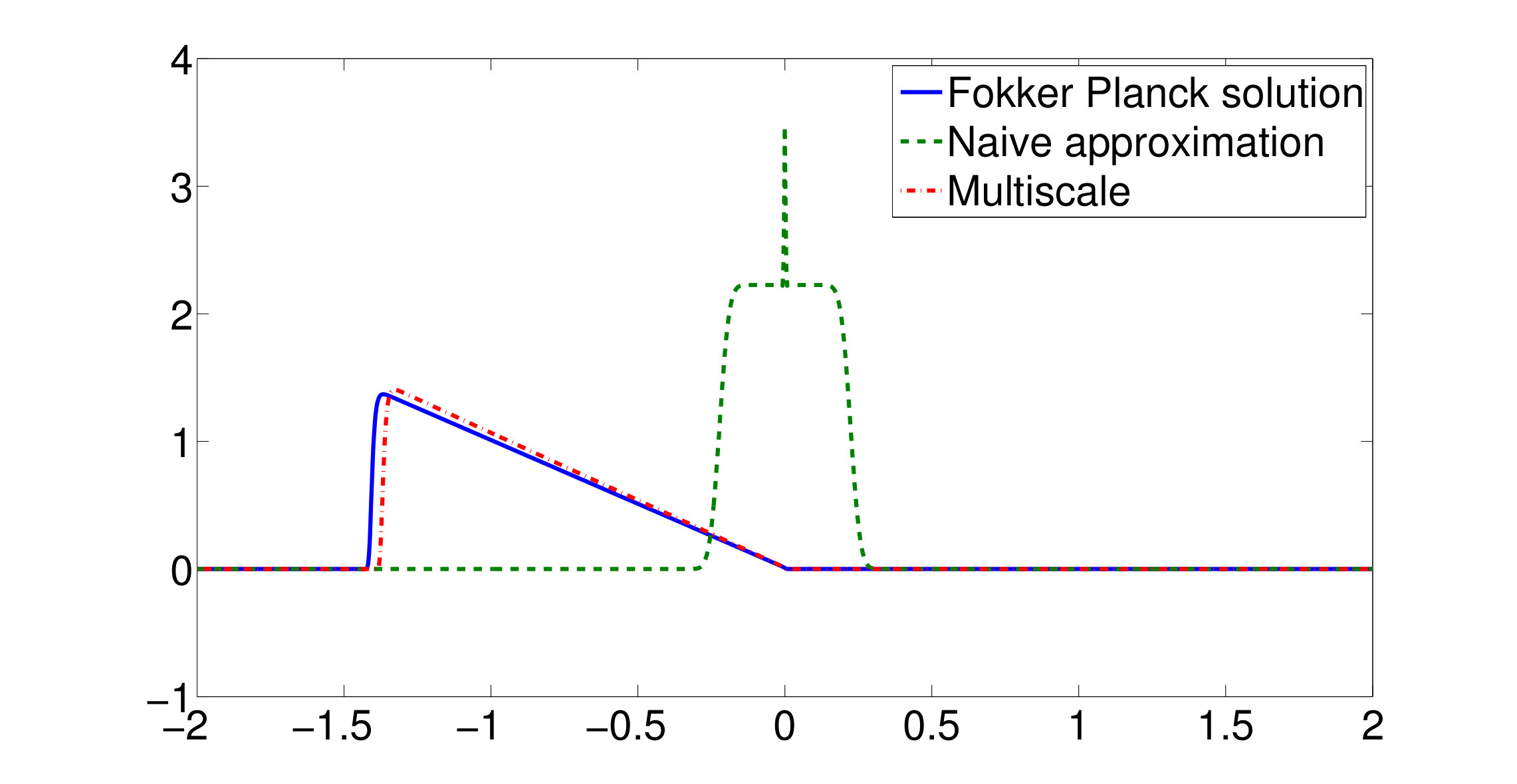 Figure 1
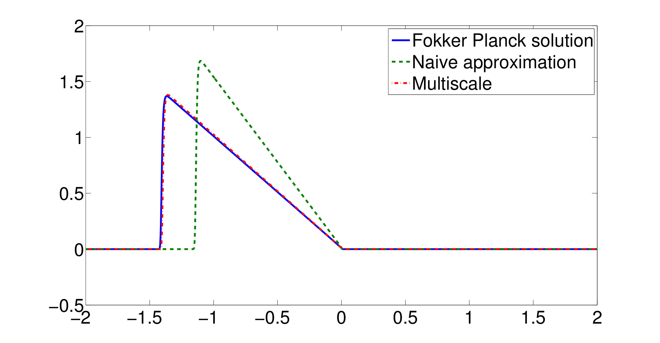 Figure 2
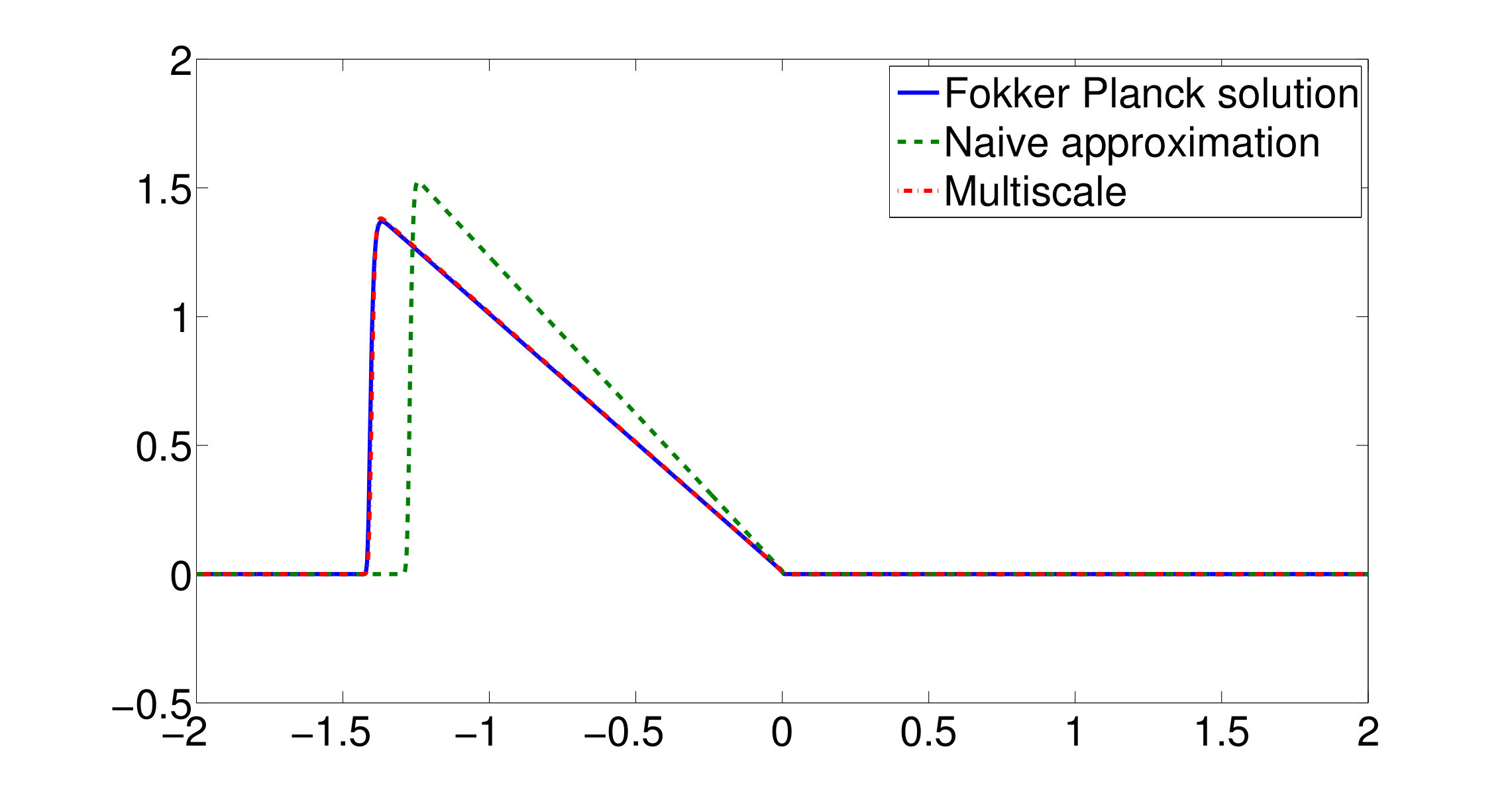 Figure 3
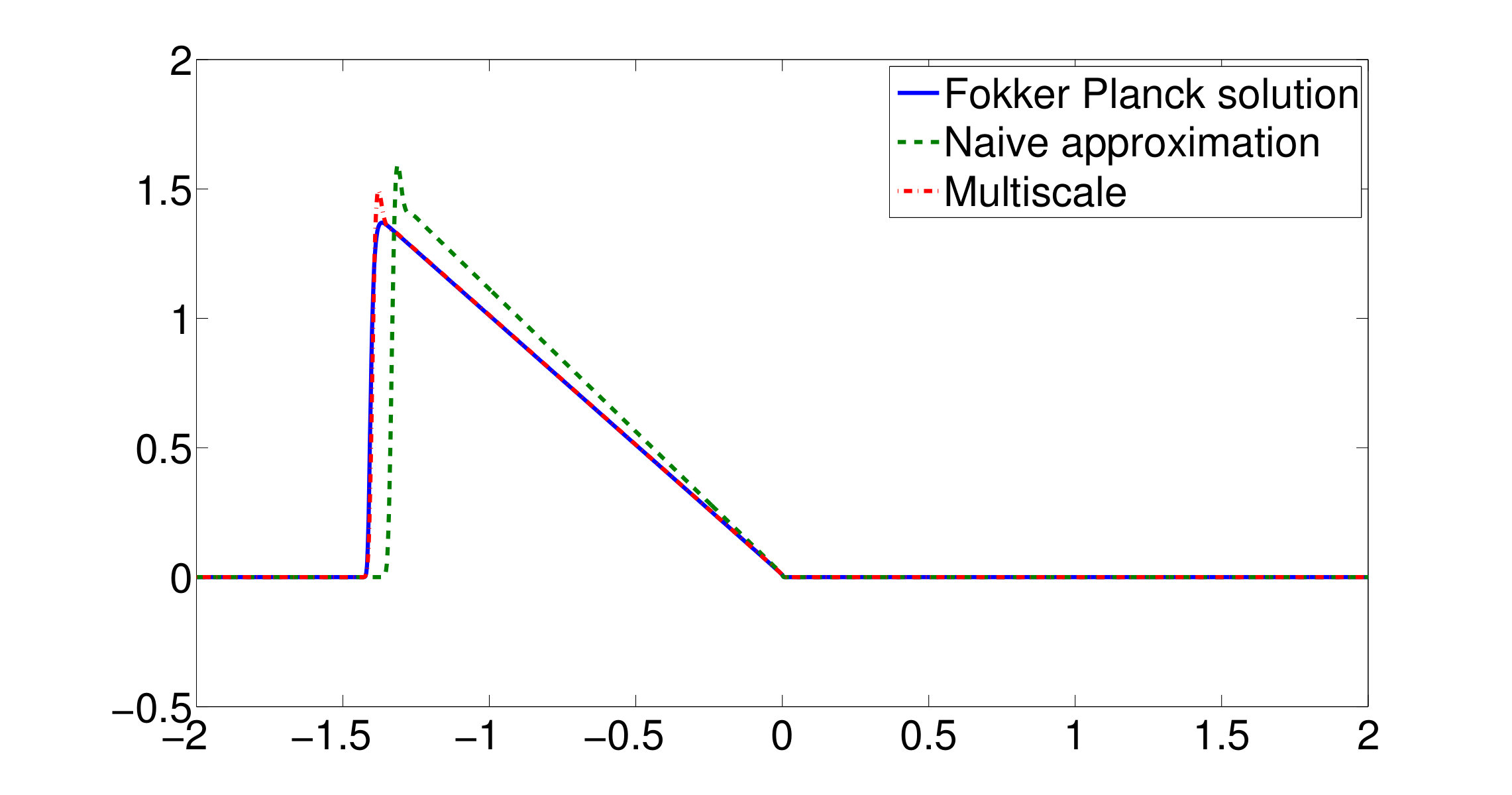 Figure 4
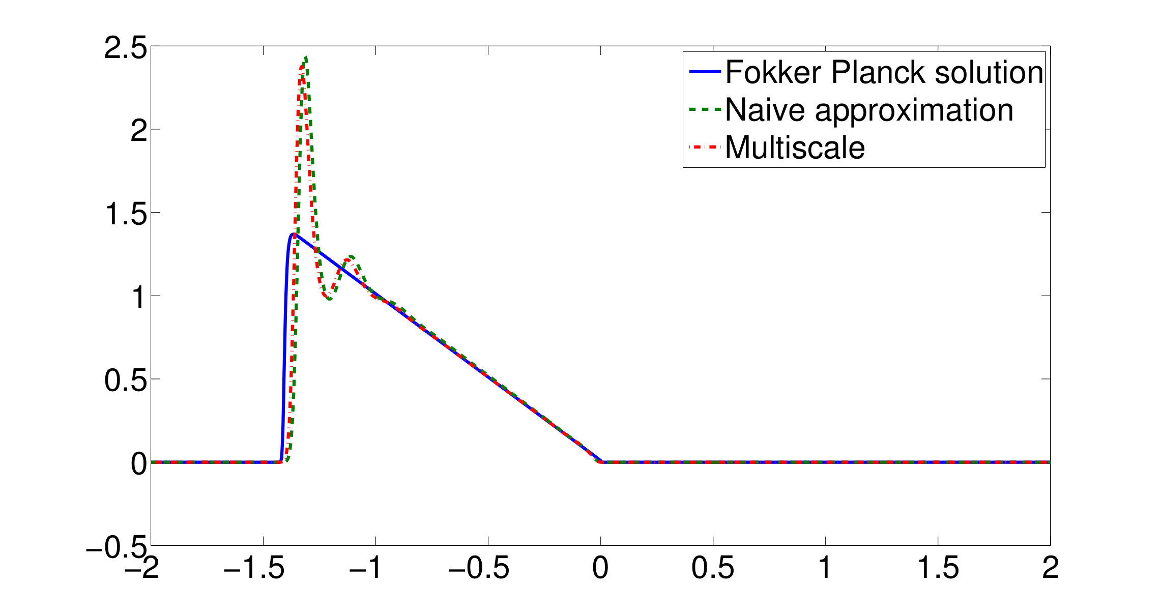 Figure 5
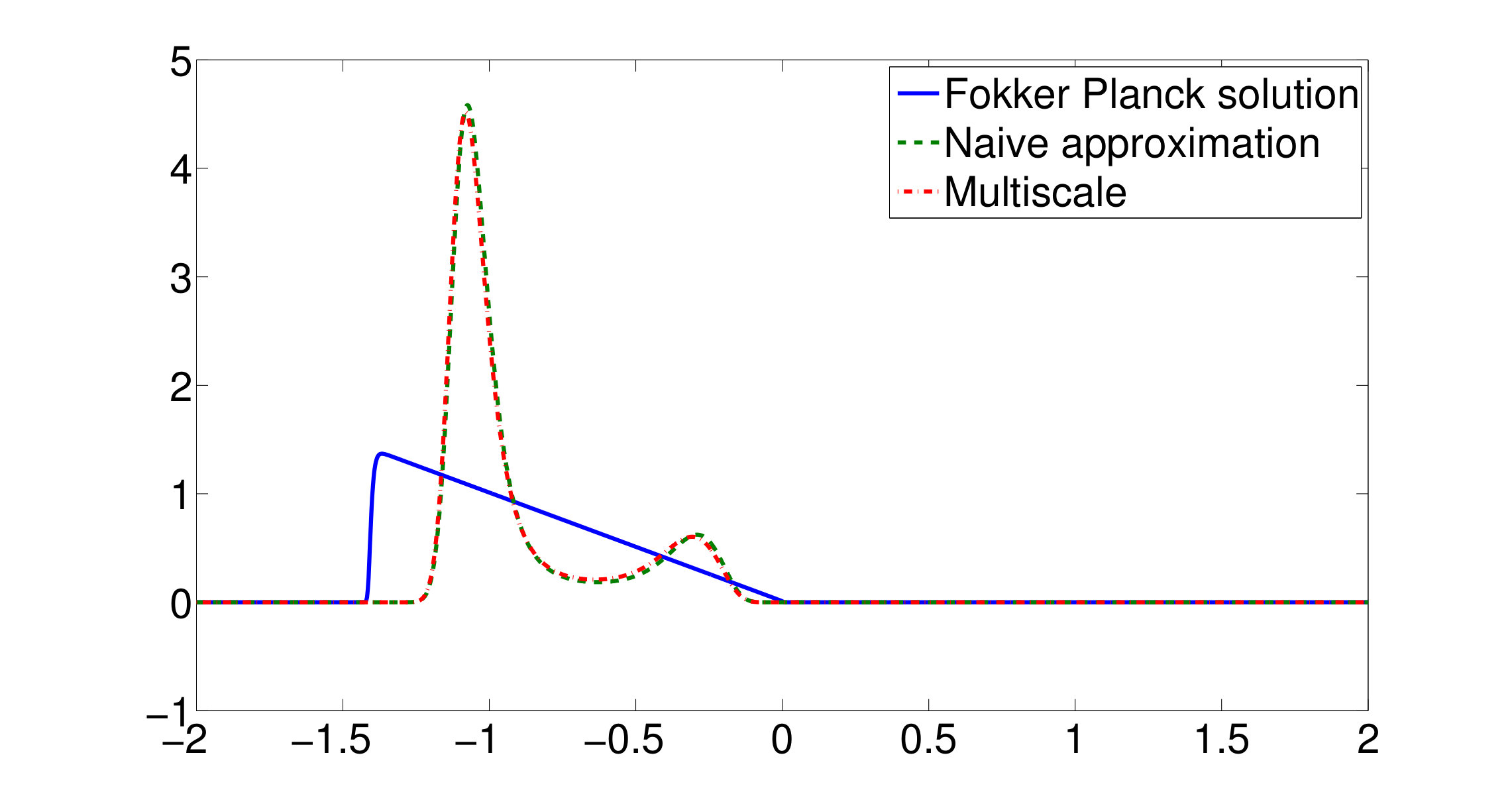 Figure 6
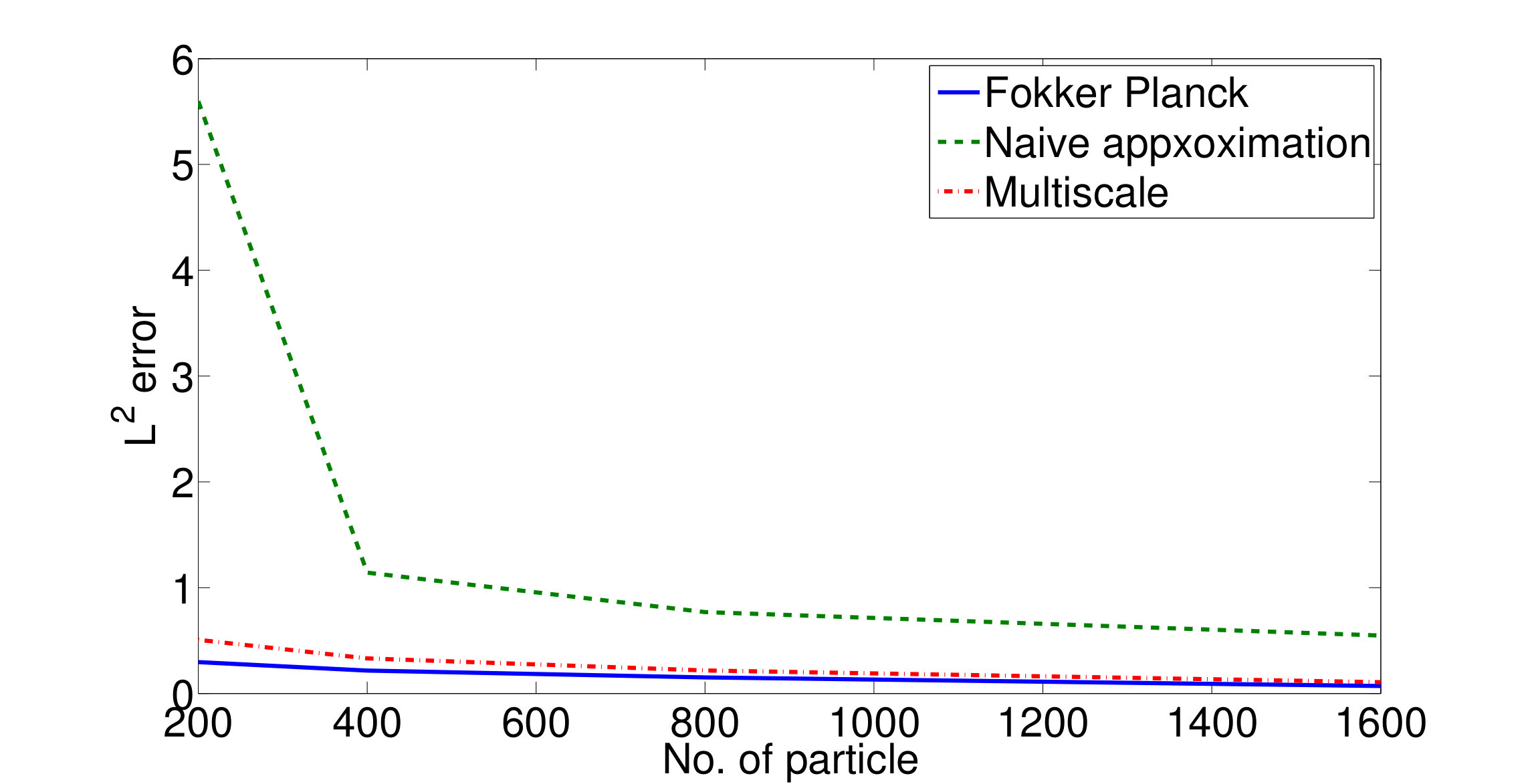 Figure 7
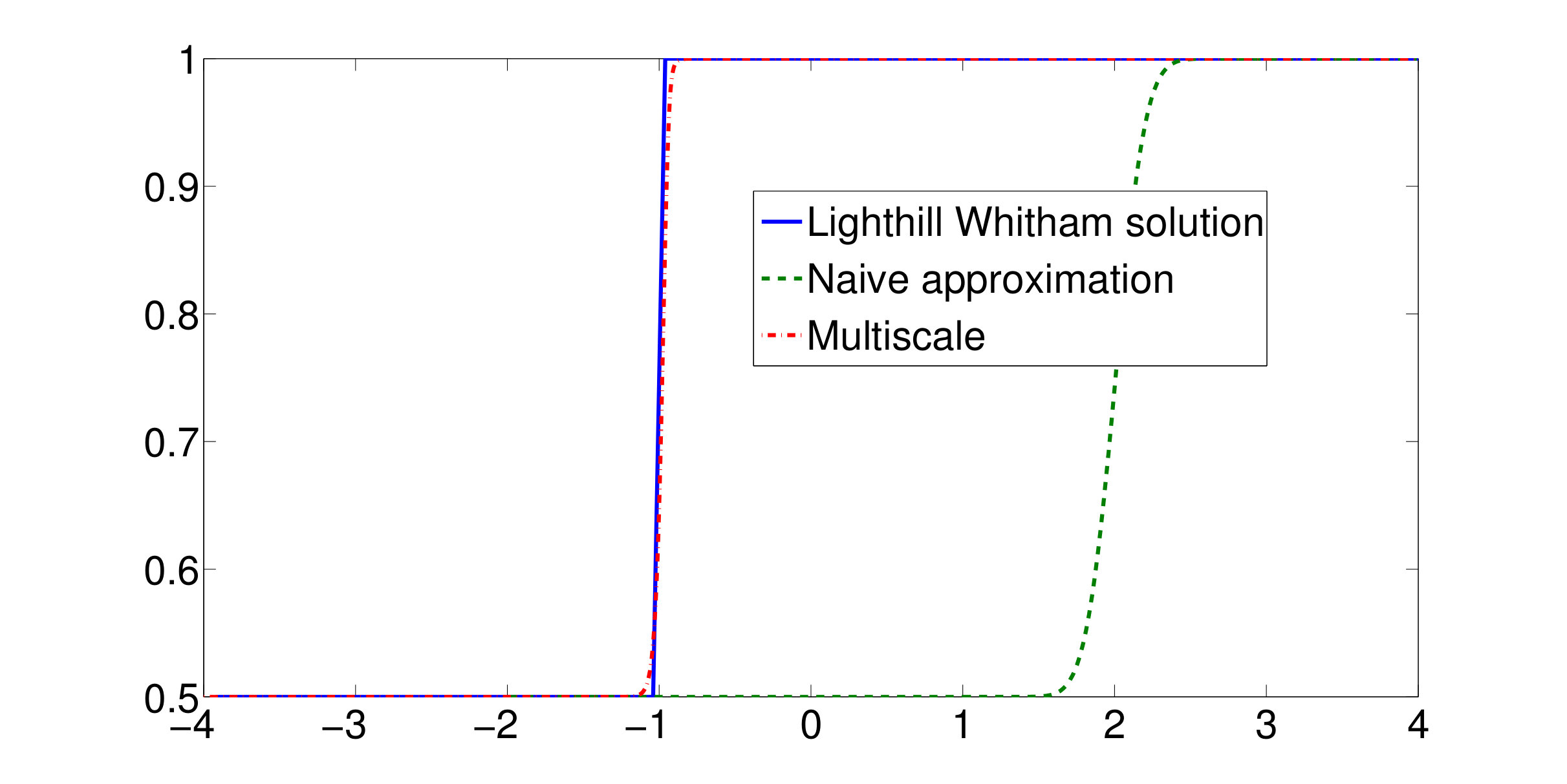 Figure 8
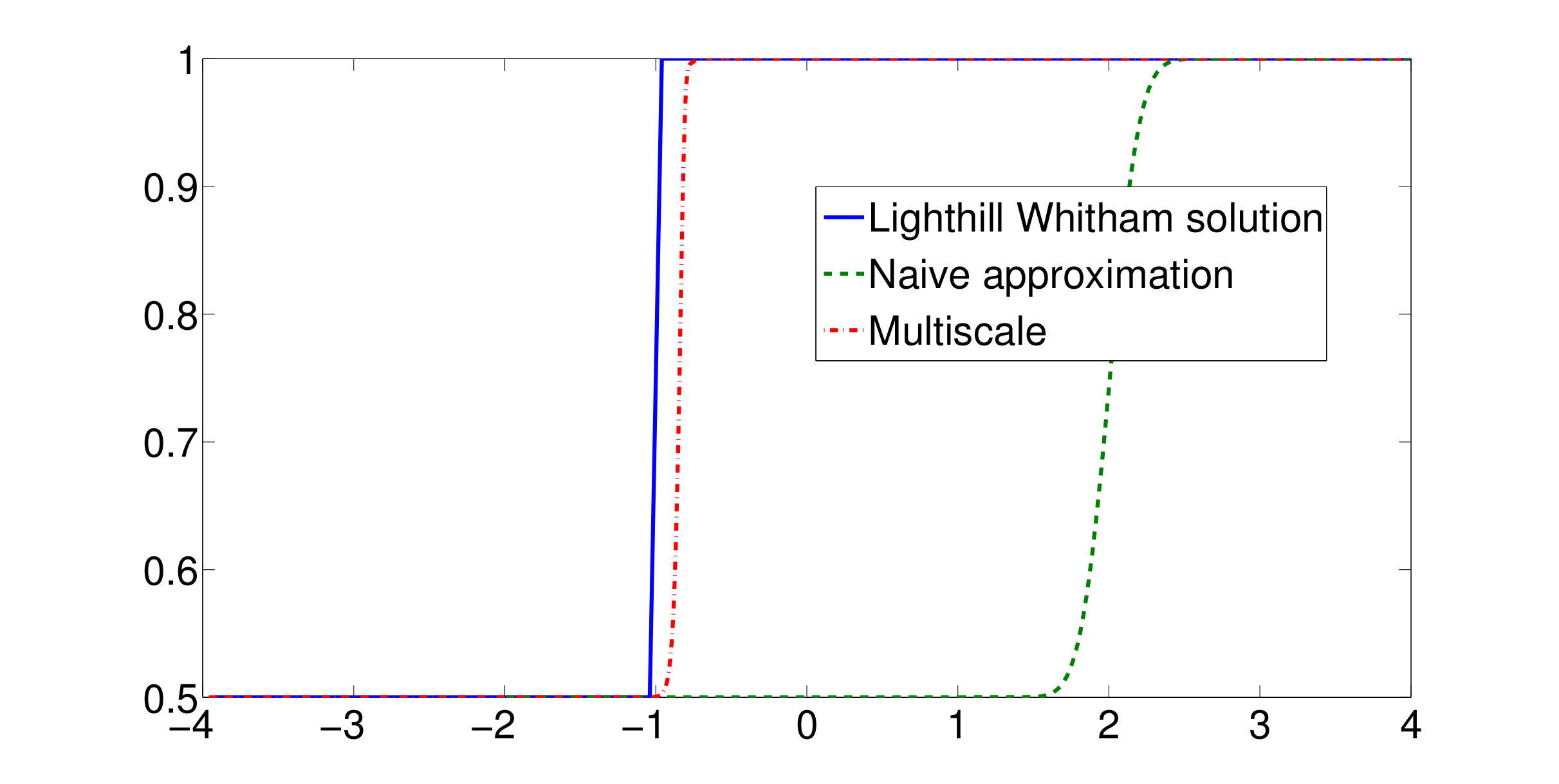 Figure 9
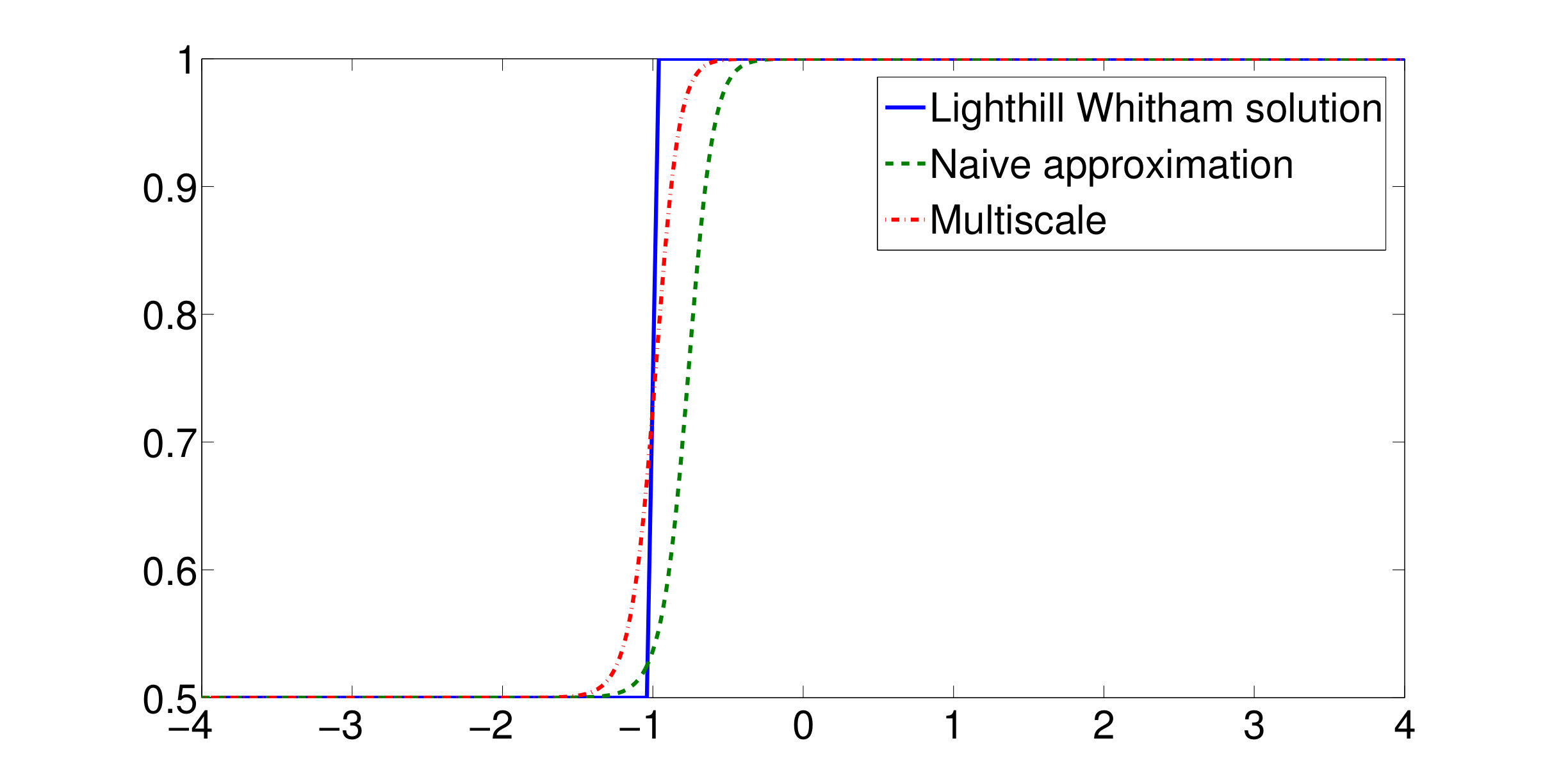 Figure 10
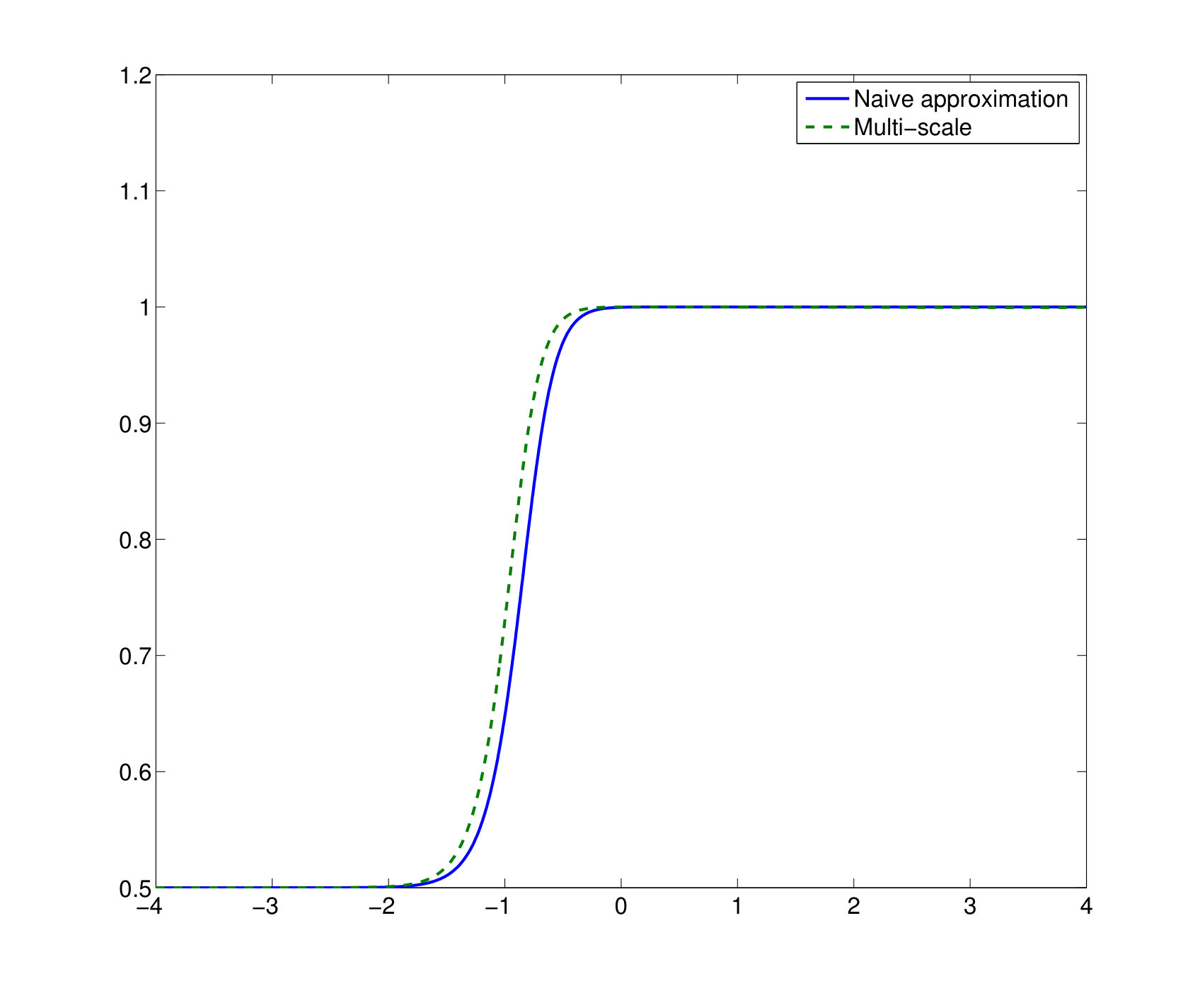 Figure 11
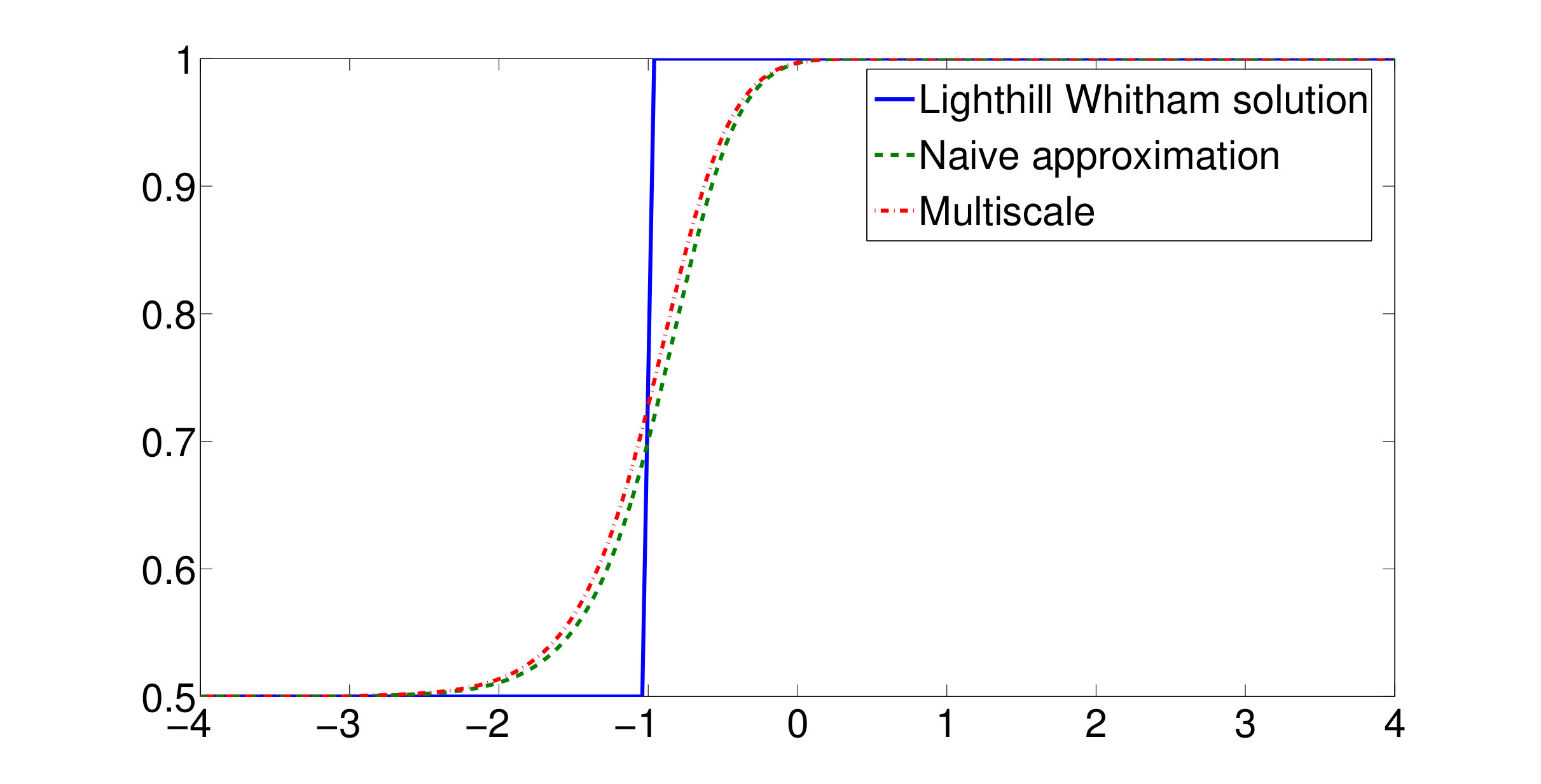 Figure 12
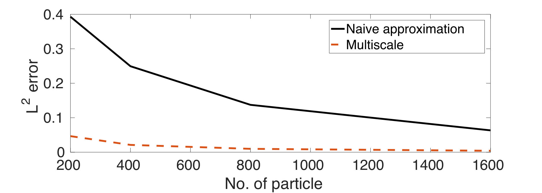 Figure 13
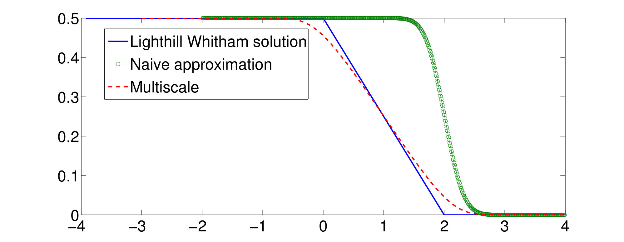 Figure 14
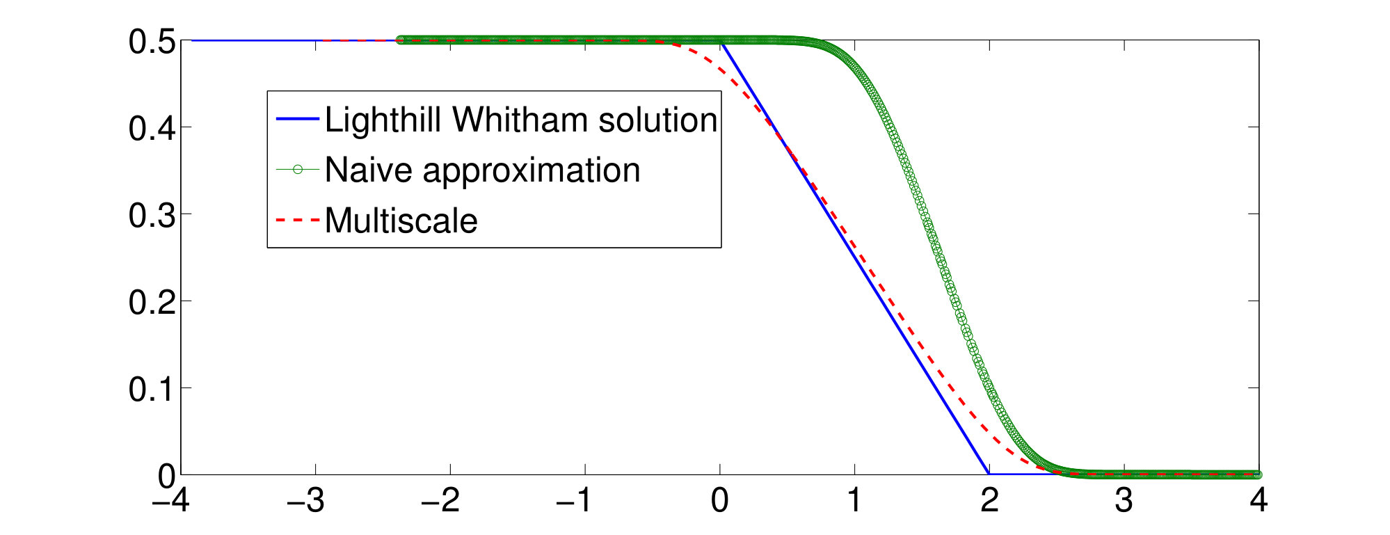 Figure 15
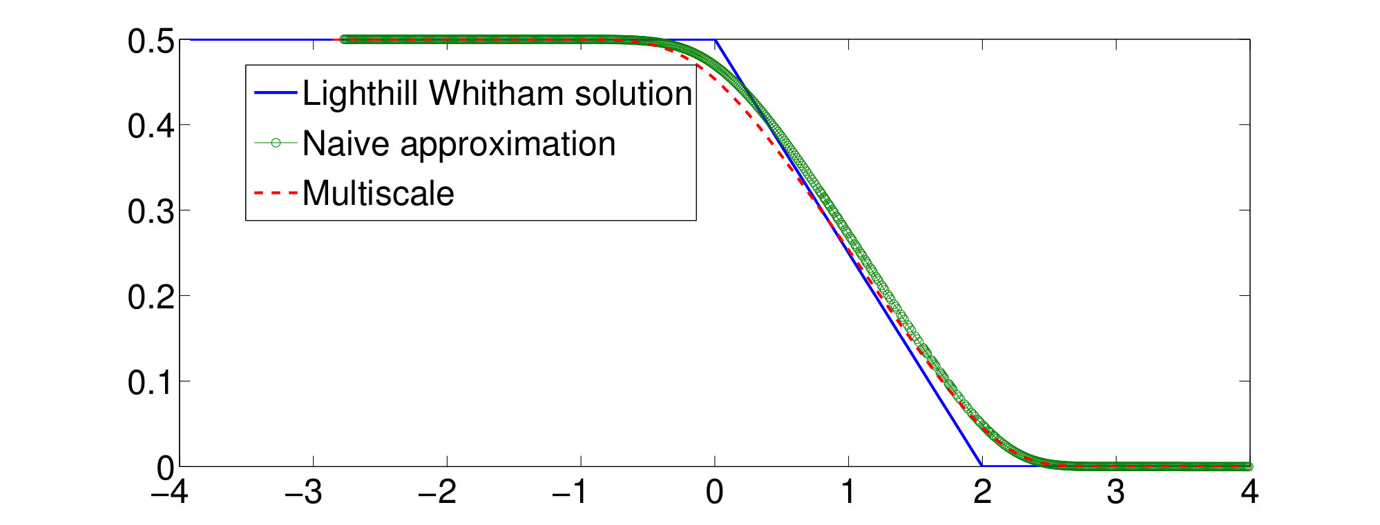 Figure 16
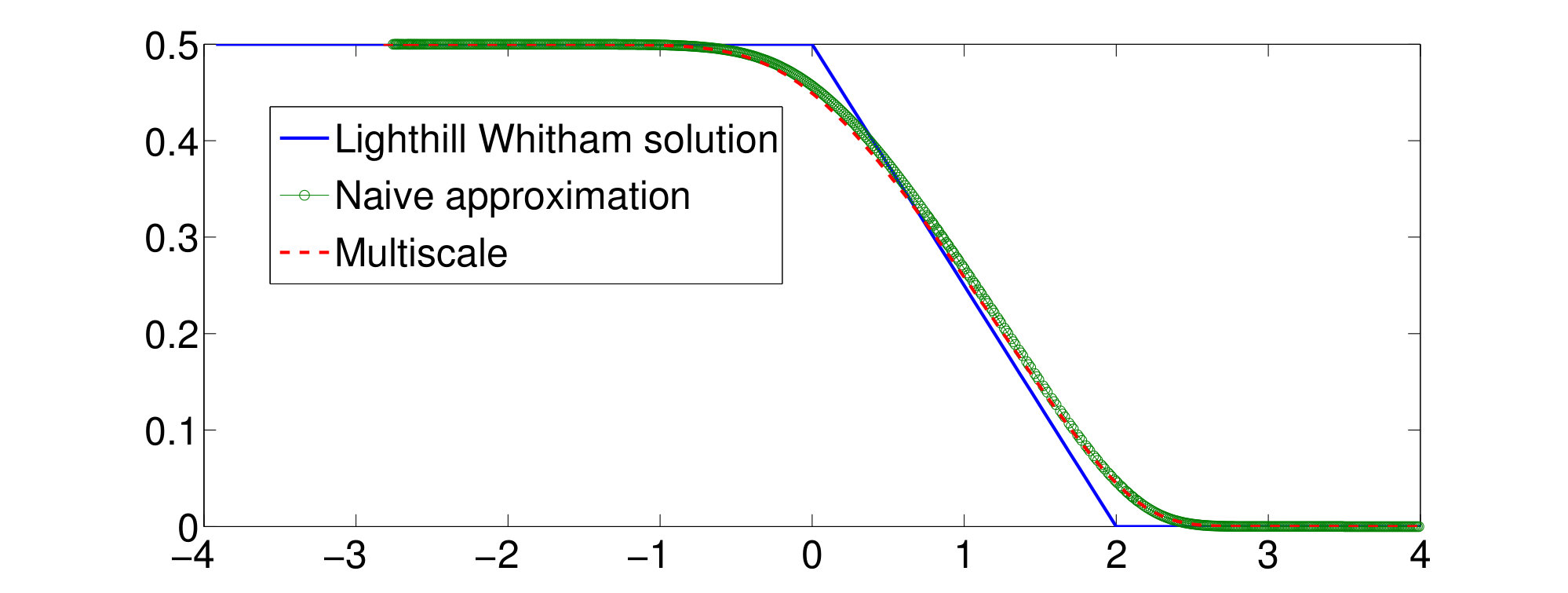 Figure 17
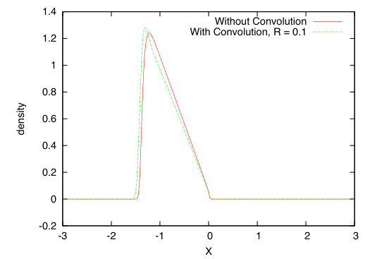 Figure 18
 Figure 19
 Figure 20
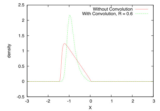 Figure 21
 Figure 22
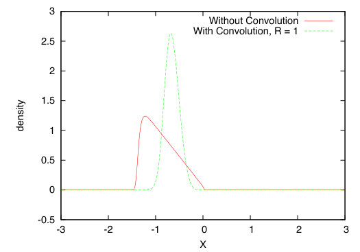 Figure 23
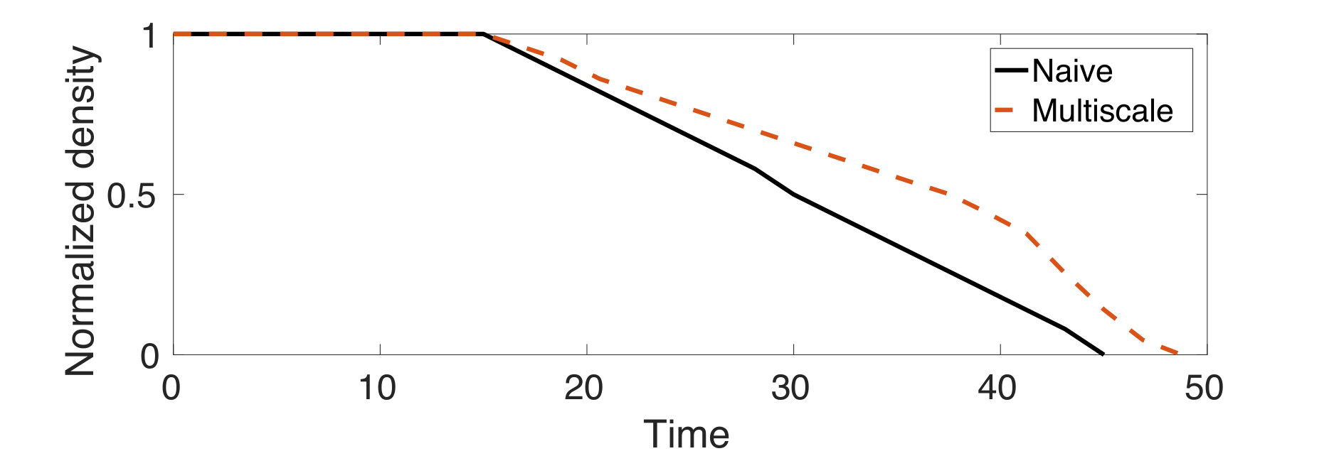 Figure 24
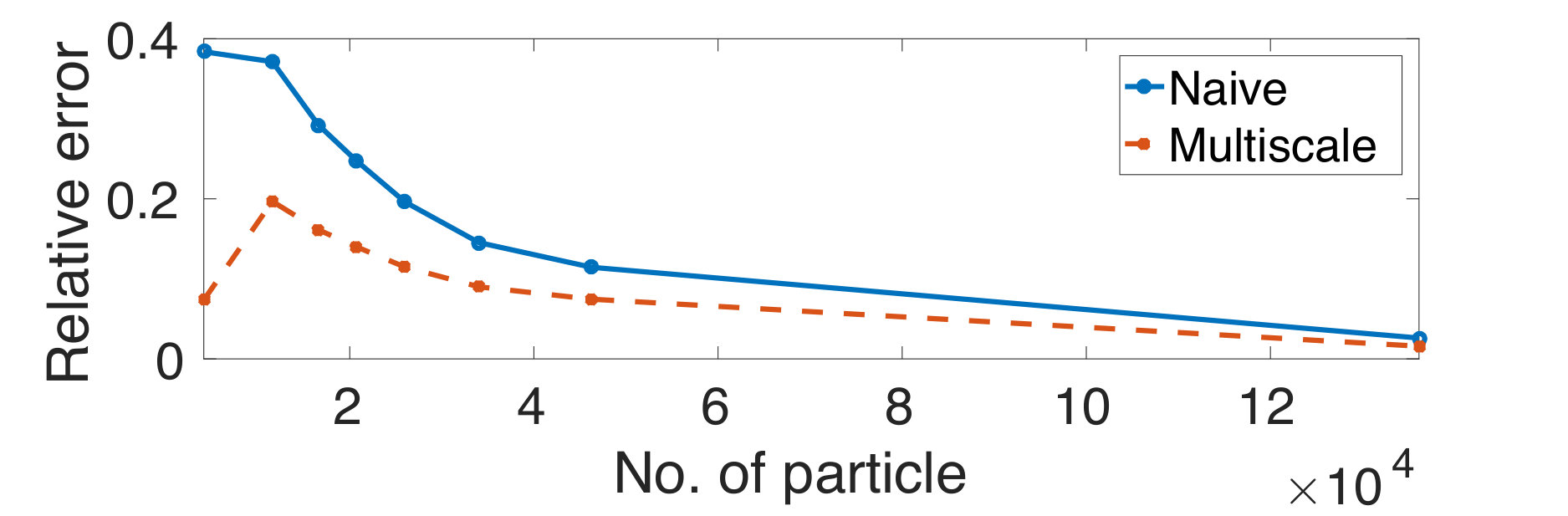 Figure 25
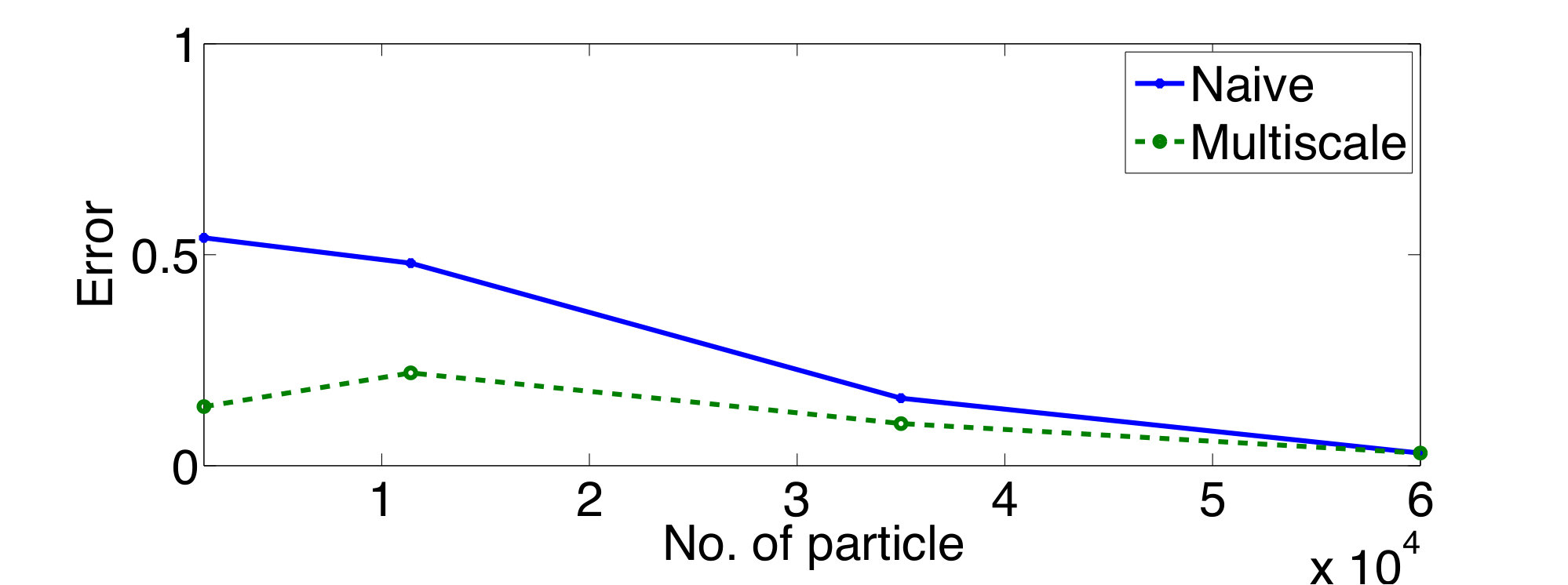 Figure 26
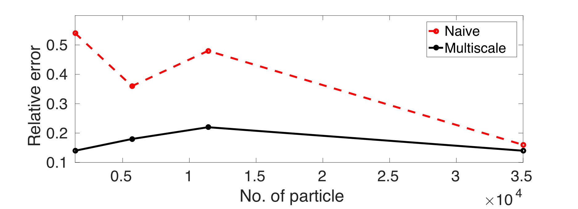 Figure 27
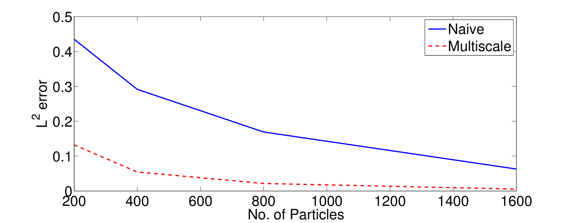 Figure 28
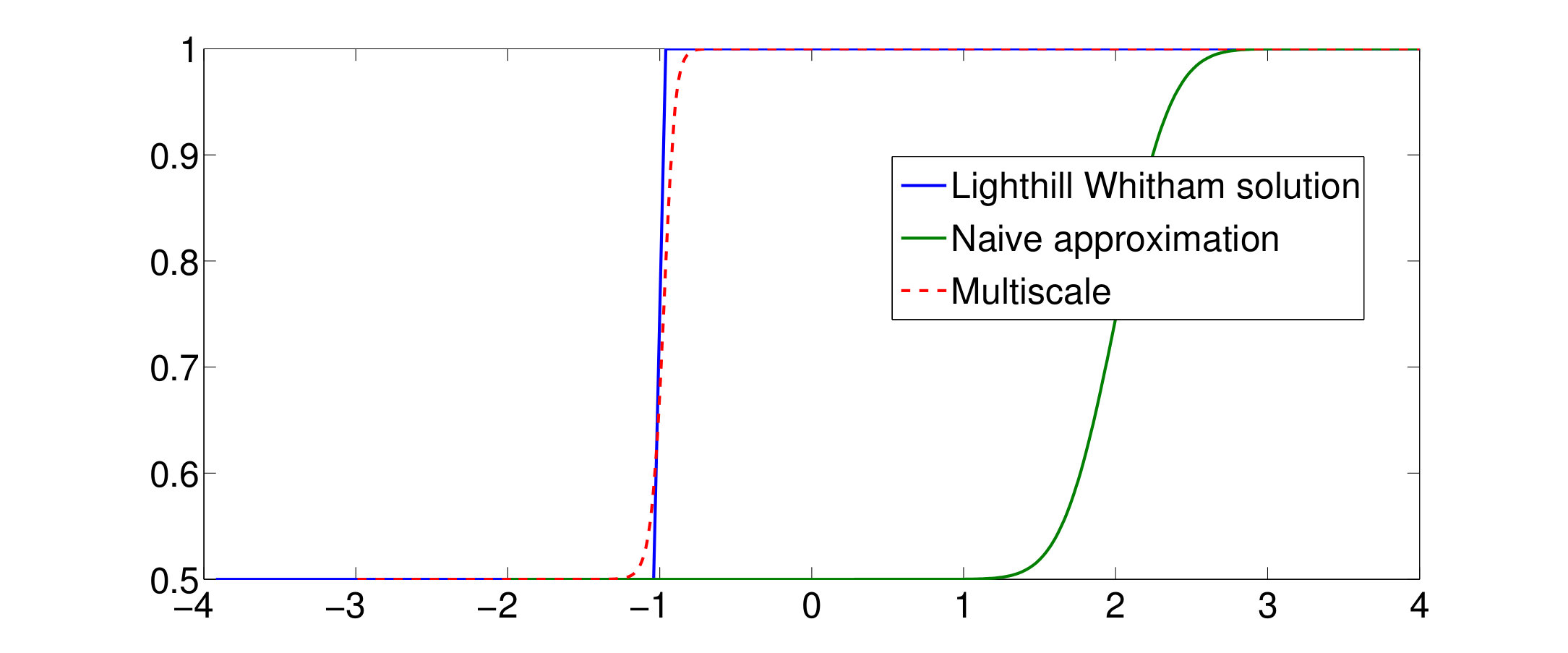 Figure 29
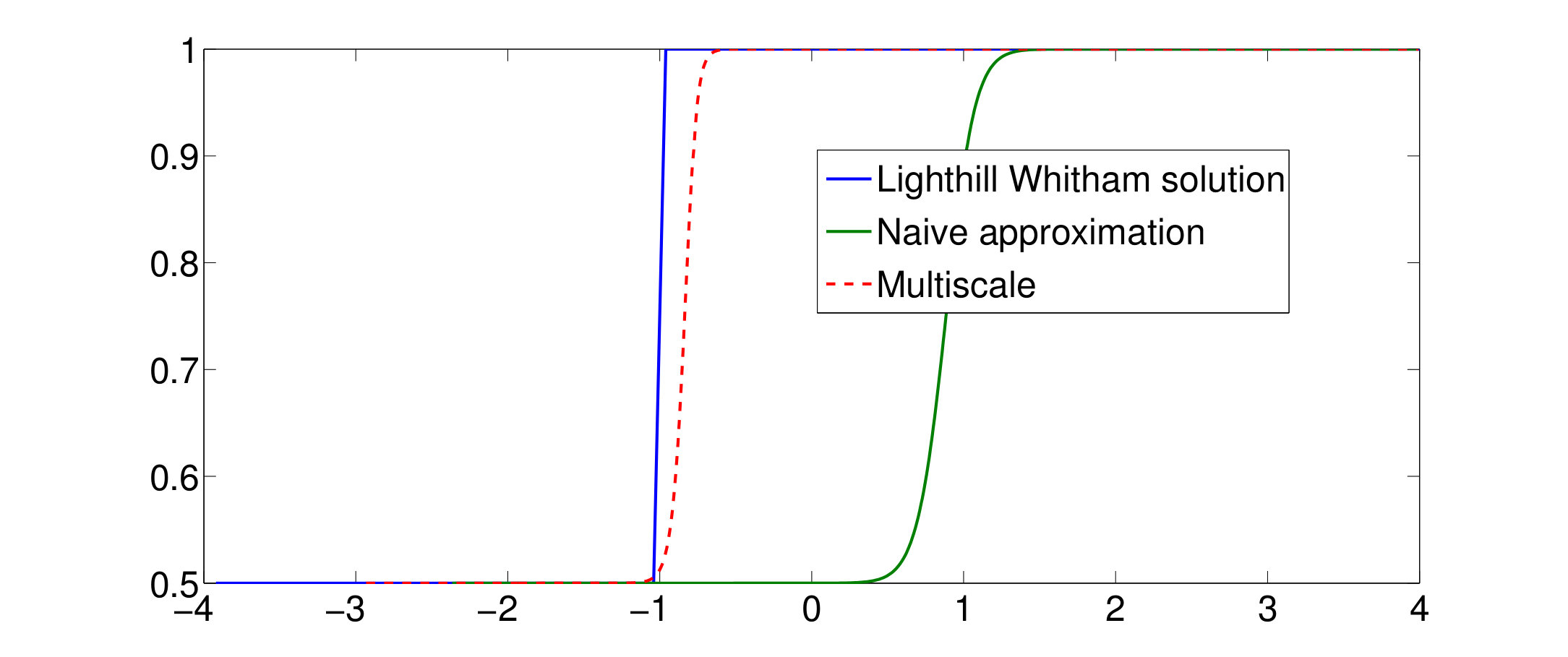 Figure 30
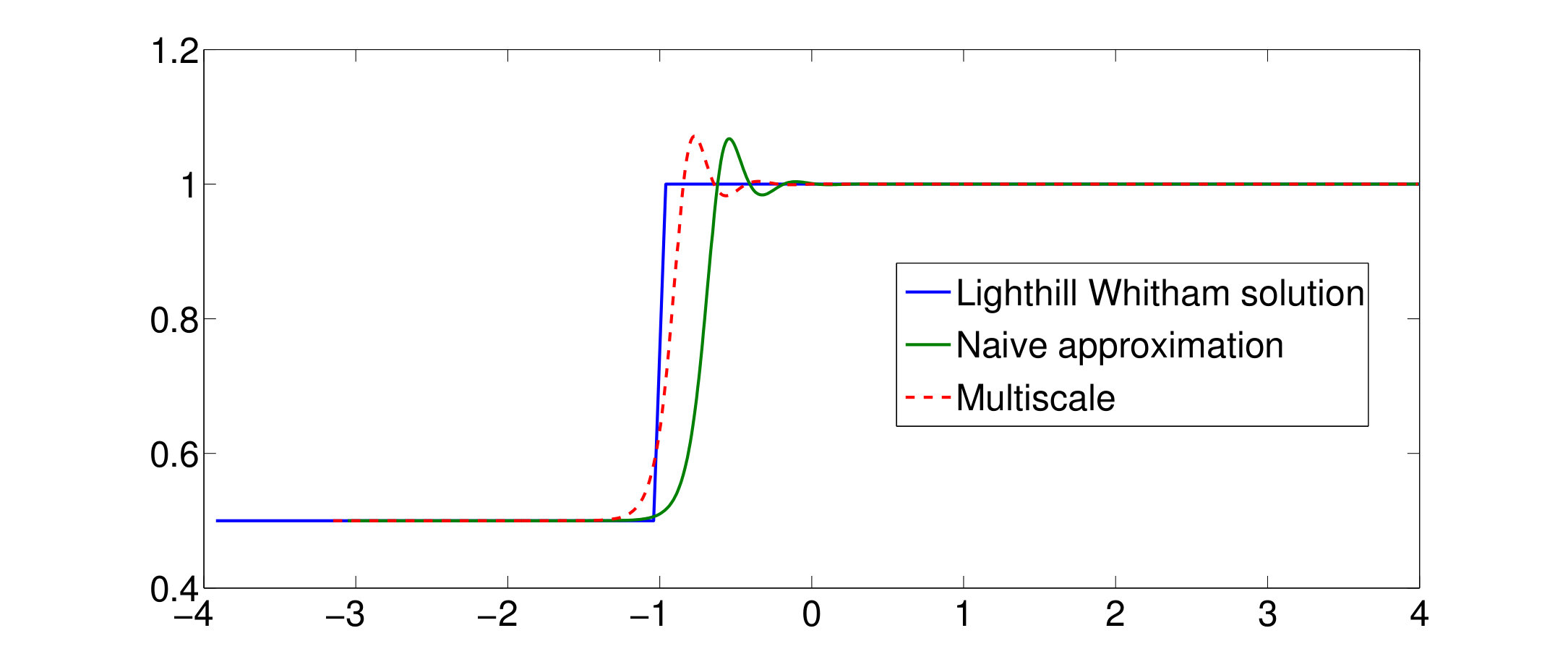 Figure 31
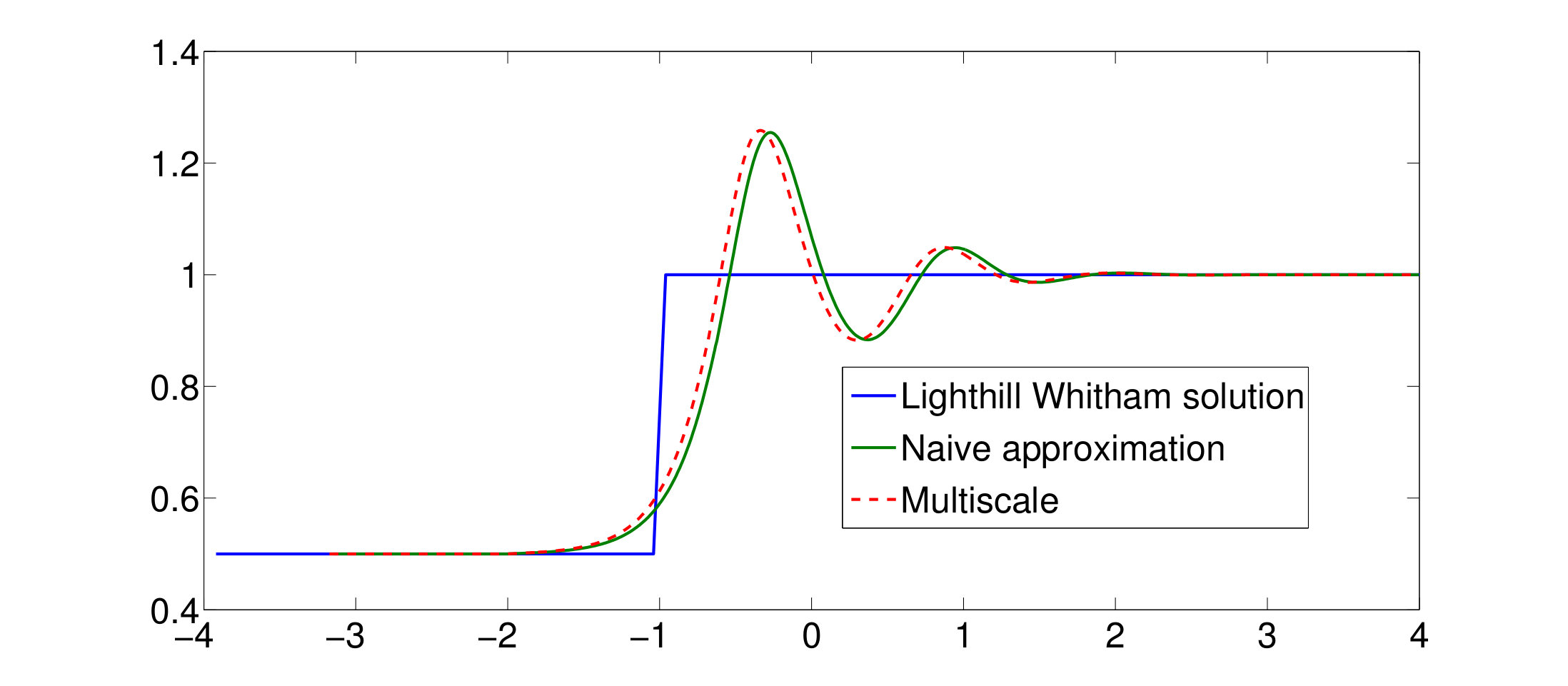 Figure 32
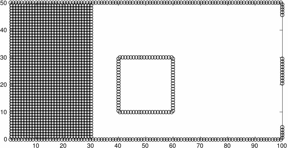 Figure 33
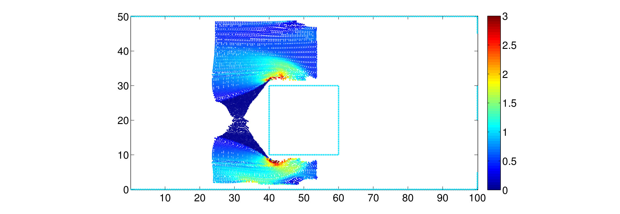 Figure 34
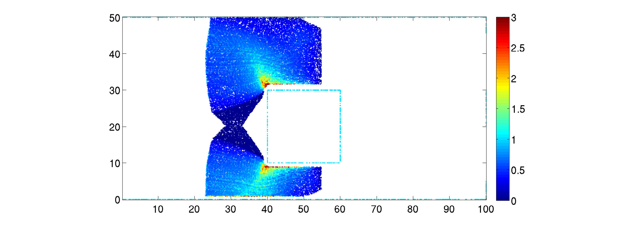 Figure 35
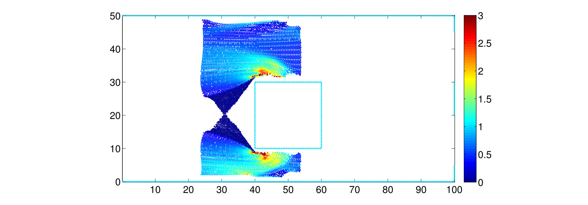 Figure 36
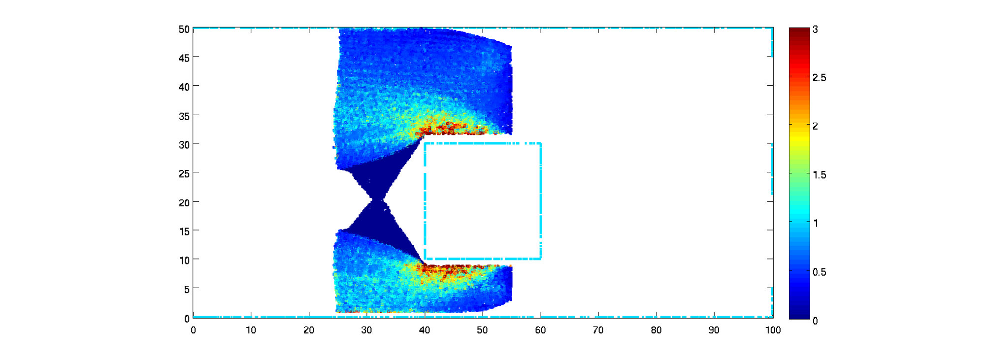 Figure 37
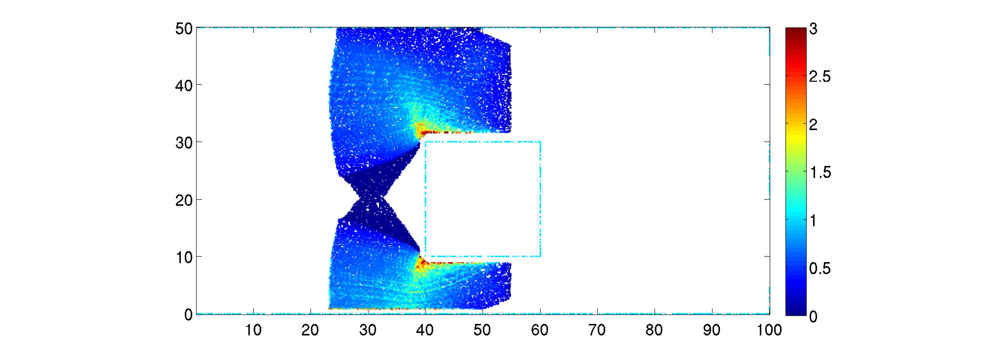 Figure 38
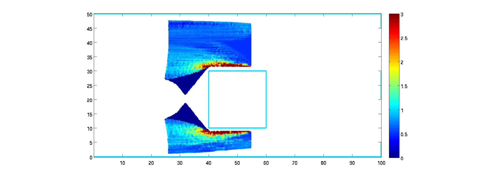 Figure 39
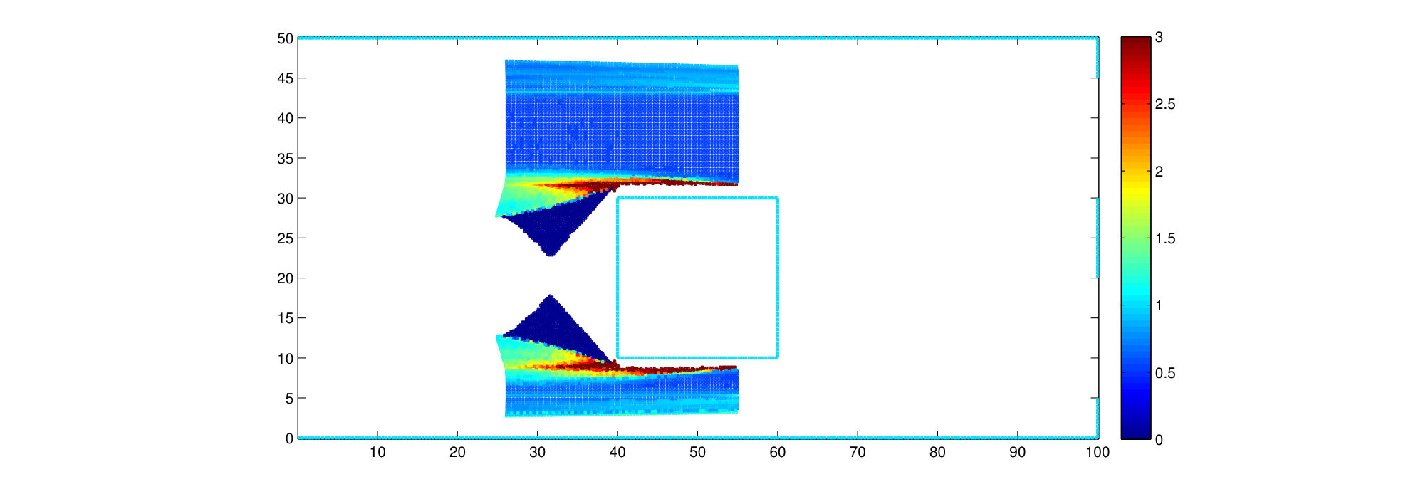 Figure 40
| Particles | Fokker-Plank | naive | multi-scale | CPU time |
|---|---|---|---|---|
| error | error | error | seconds | |
| 0.29 | ||||
| 0.21 | ||||
| 0.15 | ||||
| 0.07 |
| particles | naive | multi-scale | CPU time |
|---|---|---|---|
| error | error | in seconds | |
| 8 | |||
| 17 | |||
| 36 | |||
| 77 |
| Particles | naive | multi-scale | CPU time |
|---|---|---|---|
| error | error | in seconds | |
| initial | particles | naive | multi-scale | CPU time |
|---|---|---|---|---|
| spacing | error | error | ||
| 15 min | ||||
| min | ||||
| min | ||||
| min | ||||
| min | ||||
| min | ||||
| min |
| initial | particles | naive | multi-scale | CPU time |
|---|---|---|---|---|
| spacing | error | error | ||
| min | ||||
| min | ||||
| min | ||||
| min |
Peer Reviews
No public reviews on file for this paper yet. If you reviewed it on a platform where reviews are public (OpenReview, ICLR, NeurIPS, ICML), you can paste yours below so the community can read it here.
Videos
No videos yet. Explain this paper in a talk, walkthrough, or lecture? Add one.
A multi-scale particle method for mean field equations: the general case
A. Klar 111Technische Universität Kaiserslautern, Department of Mathematics, Erwin-Schrödinger-Straße, 67663 Kaiserslautern, Germany ({klar, tiwari}@mathematik.uni-kl.de) 222Fraunhofer ITWM, Fraunhoferplatz 1, 67663 Kaiserslautern, Germany
S. Tiwari 11footnotemark: 1
Abstract
A multi-scale meshfree particle method for macroscopic mean field approximations of generalized interacting particle models is developed and investigated. The method is working in a uniform way for large and small interaction radii. The well resolved case for large interaction radius is treated, as well as underresolved situations with small values of the interaction radius. In the present work we extend the approach from [39] for porous media type limit equations to a more general case, including in particular hyperbolic limits. The method can be viewed as a numerical transition between a DEM-type method for microscopic interacting particle systems and a meshfree particle method for macroscopic equations. We discuss in detail the numerical performance of the scheme for various examples and the potential gain in computation time. The latter is shown to be particularly high for situations near the macroscopic limit. There are various applications of the method to problems involving mean field approximations in swarming, traffic, pedestrian or granular flow simulation.
Keywords. Meshfree methods, particle methods, asymptotic preserving methods, interacting particle systems, mean field and hydrodynamic approximations, nonlinear Fokker-Planck equations.
AMS Classification. 82C21, 82C22, 65N06
1 Introduction
Interacting particle models are used in many applications ranging from engineering sciences to social sciences and biology. We refer to [12, 16, 17, 29, 30, 31] for recent work. In certain limits, for large numbers of particles, the solution of the microscopic model can be approximated by the solution of so-called mean field or macroscopic equations. For a mathematical investigation of these limits we refer to [27, 3, 8]. Microscopic interacting particle models require numerically the solution of large systems of ordinary differential equations. Many different numerical approaches can be employed for the numerical solution of the macroscopic approximations. In particular, meshless or particle methods are a popular way to solve these problems. We refer to [4, 26] for the analysis of particle methods, to [24] for a classical particle method and to [20, 51, 52, 55] for different developments of the original idea from [24].
In the present work we extend a particle method developed in [39] which is especially adapted to the solution of macroscopic mean field equations derived from interacting particle systems. The method can be viewed as a numerical transition between a DEM-type method for microscopic interacting particle systems and a meshfree particle method for macroscopic equations. For related approaches we refer to [54, 55]. In macroscopic mean-field models an interaction term appears, which is derived from the microscopic interaction term. Usually, this term has the form of a convolution integral. The particle method approximates these convolution integrals in an appropriate way not using a microscopically large number of macroscopic particles and thus allowing the use of an underresolved meshfree method. In the limit for small a method which is consistent with the asociated limit equation is obtained. For intermediate values of one obtains with this procedure an easily calculated correction term. In the present work more general particle systems and more general limit equations are considered compared to [39] where only porous media type limits have been investigated. The present investigations include for example terms leading to hyperbolic limit equations and more general applications.
The paper is organized as follows. Section 2 contains a description of the models under investigation. In particular, the macroscopic hydrodynamic models and their scalar approximations are discussed. Examples range from non-local 1D Lightill Whitham type models to non-local 2D pedestrian flow models. Section 3.1 describes the numerical method and in detail the approximation of the convolution integral. Finally, Section 4 contains the numerical results and a comparison of the methods and their computation times for the above mentioned examples.
2 The models
We consider a hierarchy of models ranging from microscopic interacting particle systems and their mean field approximations to hydrodynamic and scalar macroscopic approximations.
2.1 Microscopic and mean field equations for interacting particle system
The starting point for our model is a general microscopic model for interacting particles [37]. We define the empirical density as
[TABLE]
and consider systems of equations of the form
[TABLE]
with , , . , and a d-dimensional Brownian motion. is a sufficiently smooth, repulsive potential with support in and positive integral which is normalized to , that means
[TABLE]
We assume that approximates the delta distribution as goes to [math], . Possible extensions are given in the remarks below.
Remark 1**.**
We note that physically speaking is used here on the one hand to define the empirical density, which is used in the definition of the coefficients and . On the other hand it is used as interaction potential in the term . For the following calculations we could as well use different functions at the different places in the equation.
Example 1**.**
As an example for a repulsive interaction potential we choose for
[TABLE]
where
[TABLE]
and is the volume of the unit sphere in . The coefficients are chosen such that
[TABLE]
We note that non-symmetric potentials could be chosen as well.
Remark 2**.**
In 1D the present formulation includes one sided interaction potentials approximating the Heaviside function, i.e. . An equation of the form
[TABLE]
turns into
[TABLE]
with . Compare the systems considered in [49, 6].
Example 2**.**
For the potential in the remark above with one might choose potentials,such that is given as in example 1 or non-anticipating examples like
[TABLE]
if and [math] otherwise.
Remark 3**.**
For the following considerations, one might also consider more general attractive-repulsive potentials. For example in 1-D the following class of potentials can be considered, compare [43, 6]:
[TABLE]
where is a monotone decaying, integrable function, decaying to 0 as goes to infinity. This includes, for example, the Morse potential () used among other applications for modelling the swarming behaviour of birds, see [10]. However, for the following, the potential should lead to a spreading behaviour of the solutions goverened for long times by a diffusive equation, in our case a porous media type equation, see [45, 6, 43]. For the above class of potentials a purely repulsive potential is characterized by , see [43]. However, this is not a necessary condition for the spreading behaviour of the solution. The analysis in [43] shows that one still observes a spreading behaviour, if and , i.e. also for with . We note that in this case
[TABLE]
In dimensions the corresponding formula for a rotationally symmetric potential defined by (5) is
[TABLE]
This is larger than [math], if .
Remark 4**.**
*Velocity dependent interactions might be included, as well as further explicit dependence of and on . For example, one could include an exterior potential via . *
For going to infinity, one can derive in the limit of a large number of particles the associated mean field equation [8, 10, 3, 44]. One obtains for the distribution function of the particles the mean field equation
[TABLE]
with force term
[TABLE]
and diffusion term
[TABLE]
Here, the convolution is defined as
[TABLE]
and the density as
[TABLE]
We normalize
[TABLE]
2.2 Hydrodynamic and scalar macroscopic models
Multiplying the mean field equation with and and closing the equations by approximating the distribution function with a function having mean and variance , one obtains the continuity and momentum equations
[TABLE]
with the momentum
[TABLE]
Neglecting time derivatives and inertia terms in the -equation we approximate the velocity as
[TABLE]
and obtain the following scalar equation for the density
[TABLE]
2.3 Localized models
Since approximates for small values of a distribution, one obtains formally
[TABLE]
Thus, one obtains from the hydrodynamic equations the damped isentropic Euler equations with exterior potential
[TABLE]
From the scalar equations one obtains with the same procedure as before a nonlinear Fokker-Planck equation of the form
[TABLE]
A simple example with a solution which converges to a stationary distribution is given by the following
Example 3**.**
We consider for the following coefficients , . This leads to the microscopic problem
[TABLE]
and the scalar equation
[TABLE]
The scalar localized macroscopic approximation is
[TABLE]
with the stationary solution
[TABLE]
where is determined by the normalization . gives the well known solution of the Fokker-Planck porous media equation , see [1]. For tending to [math] one approaches a stationary distribution function, which is for a convex potential given by for and [math] otherwise. is in both cases chosen such that the normalization condition is fulfilled.
We consider further examples from traffic and pedestrian flow in one- and two space dimensions.
Example 4**.**
A simple microscopic traffic model is given as follows. We model the acceleration by choosing and . Breaking interactions are modelled by an interaction potential given by a smooth version of the Heaviside function such that , where is a smooth version of the -function. is concentrated in the negative half plane to model the fact that the interaction is essentially restricted to an interaction with the predecessors. We call a downwind potential in this case. Finally, we choose and . We obtain with
[TABLE]
*The corresponding mean field hydrodynamic equations are *
[TABLE]
and the associated scalar nonlocal viscous Lighthill-Whitham model is
[TABLE]
We remark that nonlocal Lighthill-Whitam model has been investigated in [25, 2]. There, for one-sided downwind monotone convolution kernels concentrated in the negative half plane existence and uniqueness of solutions have been shown as well as a maximum principle. In particular, the density is not exceeding the maximal density, which is in this case eqal to for suitable initial conditions. The local limits are
[TABLE]
and the Lighthill Whitham equation
[TABLE]
We note that for the one-sided downwind kernel we obtain an approximation to order in the following way. Define
[TABLE]
using we obtain
[TABLE]
This is a stable equation for . We note that using the potential defined in Example 2 we obtain . If instead of using a down-wind interaction potential we consider symmetric potentials we obtain and the approximation to order is
[TABLE]
[TABLE]
In this case we need in order to obtain a stable convergence of the solutions of equation (17) as goes to [math], compare [46]. A numerical investigation of non-local Lighthill-Whitham type equations with symmetric or upwind potentials can be found in [2]. In this case there is no maximum principle and the density might exceed the ’maximal density’.
Example 5**.**
For the 2D case we consider a model for pedestrian flow. For and we consider the microscopic model
[TABLE]
*with symmetric interaction kernel and with *
[TABLE]
where
[TABLE]
The hydrodynamic mean field limit is
[TABLE]
and the scalar limit is
[TABLE]
where
[TABLE]
The local limits are
[TABLE]
and
[TABLE]
together with
[TABLE]
which is a viscous form of the Hughes model. For a detailed modelling of the interactions between pedestrians we refer for example to [17]. For rigorous results on the Hughes model and the approximation of the model via particle systems we refer to [18, 35, 19].
In the following, our goal will be to develop a meshfree particle method for equations (7), (8) for different ranges of parameters and, in particular, for the limit equations (9), (10).
3 Numerical method
For a general description of the particle method used here and further references on the subject, we refer to [39]. Here, we concentrate on the approximation of the interaction term. We follow the approach in [39]. However, additionally to [39] we have to treat here the terms leading to hyperbolic limit equations in a suitable way.
3.1 Approximation of the interaction term using particle methods
The key point of our method is to approximate the integrals
[TABLE]
with and . We denote the Voronoi cell around particle given by the particle locations of the other particles by . denotes the volume of this cell. Then, a naive or microscopic approximation of the integral terms would be to use
[TABLE]
where is now the number of macroscopic particles used in the particle method. For small values of this results in the following problem. We consider a situation where the method is underresolved, that means where one uses a small number of macroscopic particles in contrast to the large number of microscopic particles described by the macroscopic equations. Then, the value evaluated from (23) will be zero due to the large distances between the macroscopic particles and the relatively small value of . However, the actual value of the integral will not be zero even for very small due to the corresponding ’infinite’ number of microscopic particles described by the macroscopic equations.
We resolve this problem using a higher order approximation of the integral. This yields in the limit for small a method for the limiting nonlinear Fokker-Planck equations, even if the number of macroscopic particles is still small. We use an approximation of the density given by
[TABLE]
where denotes the Voronoi cell associated to particle/mesh point and denotes the characteristic function. The approximation of the first derivative is determined via a least squares approximation using the neighbouring points. Then, we obtain for the integral (22)
[TABLE]
We approximate first the integral around the center point . To approximate the integral we distinguish between the cases and . For , we proceed as follows.
[TABLE]
This is equal to 1 for due to the normalization of the potential. For the expression is equal to 0, since
[TABLE]
Moreover,
[TABLE]
This expression is for equal to , where is the mean value of . For we obtain
[TABLE]
If then we first compute such that . Then,
[TABLE]
Thus we obtain for . For we get
[TABLE]
Finally, we compute
[TABLE]
This is equal to for . For we get
[TABLE]
The integrals over the Voronoi cells with the points as centerpoints are approximated in the following way. A simple second order approximation is given by the midpoint rule
[TABLE]
and
[TABLE]
Altogether, one obtains
[TABLE]
and
[TABLE]
with the correction factors
[TABLE]
[TABLE]
for and
[TABLE]
[TABLE]
for . We note that in order to obtain a stable approximation we have to guarantee that and are non-negative. Alltogether, we have the following algorithm
Algorithm 1**.**
For each check for particles inside the interaction-region . 2. 2.
Compute for all particles inside this region the size of the Voronoi cells 3. 3.
Use the neighbouring particles inside the neighbourhood region of radius (not only the interaction region) to compute an approximation of the first derivative . 4. 4.
Compute according to the above formulas.
Remark 5**.**
For the approximation behaves like the microscopic interaction approximation, since go to [math]. For , i.e. the underresolved situation, we have an approximation which behaves like a solution method for the macroscopic equations since go to and the other terms vanish.
Remark 6**.**
More accurate approximations of the integrals are possible at the expense of a more complicated approximation, compare [39].
Remark 7**.**
In a situation as in the above remark with we need an upwind procedure to stabilize the numerical approximation. A first order upwind procedure amounts to adding numerical diffusion proportional to In comparison, the above factor , describing the physical diffusion in case of an unsymmetric potential, is proportional to . In case , the two diffusion coefficients are of the same order. Thus, the physical diffusion is of the same order as the numerical diffusion. In order to capture the effects of the physical diffusion a higher order upwinding procedure would be necessary to reduce the numerical diffusion.
3.2 Special cases
The above formulas give for radially symmetric potentials
[TABLE]
and
[TABLE]
where is the volume of the unit sphere in . and are [math] in the radially symmetric case. Rewriting gives
[TABLE]
with
[TABLE]
for and . Moreover,
[TABLE]
with
[TABLE]
for and .
Remark 8**.**
We note that is positive, if the potential fulfills
[TABLE]
or
[TABLE]
This is the case for any repulsive potential. Also potentials like the Morse potential fulfilling the condition in Remark 3 fulfill the condition, since
[TABLE]
This expression is negative for all , if and
For the quadratic potential described in the first section in Remark 1 the above formulas give the following expressions for :
[TABLE]
with
[TABLE]
for and . Moreover,
[TABLE]
with
[TABLE]
for and . We note that . Moreover, .
In 1D this gives
[TABLE]
and the following expressions
[TABLE]
and
[TABLE]
for . In 2-D we have
[TABLE]
and the following expressions
[TABLE]
and
[TABLE]
for .
Remark 9**.**
Considering the 1-D case, the potential in Example 2, i.e.
[TABLE]
for and [math] otherwise, leads to the expressions
[TABLE]
with
[TABLE]
and for and
[TABLE]
with
[TABLE]
and for . We note that .
4 Numerical results
In this section we present a series of numerical experiments for the hydrodynamic (7) and scalar equations (8) and their localized approximations (9) and (10). In particular, we will investigate and compare the different schemes for the non-local equations for situations near the local limit. One observes the following: if a well resolved situation with a large number of particles compared to the interaction radius is considered, then the results of the multi-scale and the naive or microscopic approximation coincide. In this case the multiscale method behaves similiar to a microscopic (DEM-type) simulation. If, however, a strongly underresolved situation is considered, i.e. the number of grid particles is small compared to the interaction radius, then the numerical solution using the microscopic approximation of the integral deviates strongly from the correct solution. On the contrary, using the multi-scale method with the correction factors introduced above, a good approximation of the correct solution is obtained. In this case the multi-scale method is essentially a meshfree numerical method for macroscopic equations. Since all methods require approximately the same amount of computation time per grid-particle, the above observations can be rephrased as follows: for situations with relatively small interaction radius we obtain, using the multiscale method, a reduction in computation time by several orders of magnitude. On the other hand, for relatively large interaction radius, the computation times of the microscopic approximation and of the multiscale method are similar.
4.1 Numerical results in 1-D
4.1.1 Test case (Example 3)
We study 1-D movement of the particles under the influence of a confining potential. The equations are described in Example 3. More precisely, we look at equations (11) and its limit equation (12). The interaction potential is given by (3). We consider the case of small . The porous media case has been treated in Ref. [39]. We choose and . We choose different values for the interaction radius . For this example the particles are assumed to be distributed on a fixed equidistant grid, i.e. we use here an Eulerian approach. Situations with arbitrary particle locations and a Lagrangian approach are considered in the following subsections. The initial density is given by for and [math] elsewhere. As time proceeds the density converges to a stationary solution depending on the value of . For the localized limit equation this stationary solution is for small values of approximated by for and otherwise, such that . In order to obtain the steady state solution we have solved the equation until .
In Figure 1 we plot the solutions for a fixed number of particles and different values of , considering in this way the different algorithms in the well-resolved, in intermediate cases and in the underresolved case. We plot the limiting Fokker-Planck solution and the microscopic and multi-scale solutions. In the well resolved case, i.e. here for larger values of , the microscopic approximation of the integral and the multi-scale solution give similiar results deviating from the solution of the limiting Fokker-Planck equation. For the under-resolved case, for smaller values of , the microscopic approximation does not give the correct results as discussed above, in contrast to the the multi-scale method. In particular, one observes that using the microscopic discretization for an underresolved situation, the numerical evolution terminates before the stationary state is reached, if the compact supports of the interaction kernels of the finite number of particles do not overlap any more.
Finally, we investigate the convergence rate of the method numerically. We consider a situation near the localized limit with , where the limit equation gives the correct solution up to order and is used as the reference solution. We compute the error of the particle methods for the scalar model (11) comparing the numerical results to the numerically determined stationary solution. The scalar problem is solved with microscopic and multi-scale approximation of the interaction term. In Figure 2 and Table 1 the -errors versus the number of particles are plotted. One observes the deterioration of the method using the microscopic approximation of the interaction term for smaller numbers of particles. The multi-scale method is able to treat all ranges with a similiar accuracy. We remark that the computation time for the different methods is approximately the same for the same number of particles. Looking at Table 1 we observe that the multiscale method with particles yields for the present example the same error as the microscopic method with particles. Thus, the computation time for the naive, microscopic method is approximately an order of magnitude larger than the time for the multi-scale method.
4.1.2 Non-local traffic flow (Example 4)
We consider equations (14) and (16) with different initial conditions and different choices of the interaction potential. For this example, we consider a fully Lagrangian approach. First we consider a symmetric potential as in Example 1 and initial conditions leading to a rarefaction wave solution. We choose
[TABLE]
The solution of the limit equation (16) is a rarefaction wave
[TABLE]
We choose and . In Figure 3 the rarefaction solution is compared at time for the scalar model (16) and for (14) with microscopic interaction approximation and multi-scale approximation. We use a fixed number of particles and an interaction radius ranging from to . One observes a good coincidence of microscopic and multi-scale approximation for large and a stronger deviation, the smaller the value of is chosen. In this situation the influence of larger values of on the exact solution is a small increase of the smearing of the solution. We note that in this situation using a one-sided downwind interaction potential as in Example 2 and gives similar results.
Second we consider a shock solution of the Riemann problem for equation (14) and (16). The initial values are now chosen as
[TABLE]
The solution of the limit equation (16) is a shock
[TABLE]
We consider first the case of a one-sided downwind potential chosen as in Example 2 and chose . In Figure 4 we compare again different values of for a fixed number of particles. We observe, that in the well resolved case for larger values of the microscopic approximation and the multi-scale solution give a smeared out shock solution deviating from the solution of the limiting equation which is a moving shock. For the under-resolved case with smaller values of , the microscopic approximation does not give the correct results, in particular, the speed of the computed wave is wrong and equal to the one of the advection problem obtained after setting in (14) equal to [math]. This is in contrast to the multi-scale method which computes the correct wave speed.
For the investigation of the convergence of the method we consider a situation with . The scalar problem is solved with microscopic and multi-scale approximation of the interaction term. We compute the error of the different methods for different numbers of grid-particles comparing the numerical results to the numerical solution of (14) determined with a fine grid with . For particles the difference between multi-scale and naive method is again of the order . In Figure 5 and Table 2 the -errors versus the number of particles are plotted. One observes again the deterioration of the method using the microscopic approximation of the interaction term for smaller numbers of particles. The multi-scale method is able to treat all ranges with a reasonable accuracy for the first order method.
Similiar to the example in the last subsection comparable errors are obtained using particles and a computation time of for the multi-scale method and particles and a computation time of for the microscopic method. This yields again an order of magnitude gain in computation time.
Finally we investigate the above example with a symmetric interaction potential and a regularization . In Figure 6 we compare again different values of for a fixed number of particles. We observe, as before that in the well resolved case for larger values of the microscopic approximation and the multi-scale solution give an oscillating solution deviating from the moving shock solution of the limit equation. For the under-resolved case with smaller values of , the microscopic approximation does not give the correct results as in the case of the downwind potential, whereas the multi-scale method computes the correct solution.
For the investigation of the convergence of the method we consider as before . We compute the error of the particle method for different numbers of grid-particles comparing the numerical results to the numerical solution of (14) determined with a fine grid with . The scalar problem is solved with microscopic and multi-scale approximation of the interaction term. In Figure 7 and Table 3 the -errors versus the number of particles are plotted. One observes a similiar behaviour as in the non-symmetric potential case. We remark that the method developed here is still working in the present case, since we have regularized the equations with obtaining a dissipative limit. For much smaller, the limit would be dominated by dispersion and the method is not supposed to work more efficienly than the naive, microscopic approximation.
4.2 Comparison of numerical algorithms in 2D
In this section we solve the hydrodynamic system (18) using the multi-scale algorithm and the algorithm with naive, microscopic evaluation of the integral in 2D. We compare the results with each other and with the local hydrodynamic problem (20). We consider a fully Lagrangian approach.
4.2.1 Hydrodynamic system for test case
We consider a two dimensional domain . We initially generate particles in . We simplify the hydrodynamic system (18) considering a fixed vector The maximal velocity is and the maximal density is chosen as . A symmetric interaction potential and are chosen. Moreover, . We use particles and the interaction radius equal to . The initial condition is given by
[TABLE]
In Figure 8 a.) the solutions of the nonlocal equations (18) with microscopic and multi-scale interaction aproximation for the interaction radius are plotted. Moreover, the time development of the normalized total mass in the domain is plotted for microscopic and multi-scale interaction approximation in Figure 8 b.).
In Table 4 we compute the error and the CPU times of naive and multi-scale method for different numbers of grid-particles, see also Figure 9. The reference solution is computed by using a spacing of and approximately particles. For this very fine resolved case the difference of naive and multi-scale solution is approximately equal to . One observes in this physical situation a smaller but still relevant gain in computation time.
4.2.2 Hydrodynamic systems for pedestrian flow (Example 5)
In our final example we investigate the hydrodynamic systems (18) and (20). Compared to the last subsection we consider a more complicated configuration defined in Ref. [40], compare also ([22]), and a full coupling to the eikonal equation.
Pedestrians are initialized on the left of the domain and evacuated towards the exits on the right as shown in Figure 10. As initial value we choose a constant value of in the region . In the center of the computational domain an obstacle is located. For the eikonal equation we use on the two exits and on all walls as boundary conditions.
We choose the maximum velocity and the maximum density . In this case, we vary the initial average distance between grid points from to , i.e. the number of grid particles varies between and . Moreover, we choose the following parameter: .
First we consider an underresolved situation with relatively small value and , i.e a number of particles of approximately . In Figure 11 we plot the solution at fixed time using the localized equation and the nonlocal equation with multiscale method and microscopic integration. In this case the solution computed via the multi-scale method and the one computed from the localized equation coincide, whereas the microscopic method gives strongly different results. In Figure 12 we show a comparison of solutions obtained from the microscopic scheme with decreasing discretization sizes or increasing number of particles.
Figure 13 considers a well-resolved case with and . In this case we observe good coincidence of the solutions of microscopic an multi-scale approximations.
Finally, in Table 5 and Figure 15 we compute the error and the CPU times of naive and multi-scale method for different numbers of grid-particles. The errors are determined along a line with and . The relative -errors are given as well as the computation times in minutes. The reference solution is computed by using a spacing of and approximately particles. For this fine resolved case the difference of naive and multi-scale solution is approximately equal to . Looking at Table 5 and the multiscale error with particles and the naive error with particles one observes in this more complex situation a gain in computation time by more than an order of magnitude. comparing the naive computation with particles with the multi-scale simulation with particles there is still a gain of an order of magnitude.
5 Conclusion and Outlook
We have extended a multi-scale meshfree particle method for macroscopic mean field approximations working uniformly for a large range of interaction parameters . The well resolved case for large is treated as well as underresolved situations for small values of . The method can be considered as a numerical transition from a microscopic system simulation to a macroscopic averaged simulation. Application of the method are shown for pedestrian flow simulations. The potential gain in computation time compared to a microscopic simulation is depending on the situation under consideration wit a potential gain of several orders of magnitude. In the situations considered in this paper we have obtained a gain in computation time of approximately one order of magnitude. Situations with more complex geometries or moving boundaries as well as the investigation of attractive-repulsive potentials will be treated in future work, compare [41].
Acknowledgment
This work is supported by the German research foundation, DFG grant KL 1105/20-1.
The reference list from the paper itself. Each links out to its DOI / PubMed record.
- 1[1] D.G. Aronson, Regularity properties of flows through porous media . SIAM J. Appl. Math. 17, (1969), 461-467.
- 2[2] S. Blandin and P. Goatin, Well-posedness of a conservation law with non-local flux arising in traffic flow modeling . Numer. Math., 132, 2 (2016), 217-241
- 3[3] W. Braun, K. Hepp, The Vlasov Dynamics and Its Fluctuations in the 1/N Limit of Interacting Classical Particles . Commun. Math. Phys. 56, (1977), 101-113.
- 4[4] T. Belytschko, Y. Guo, W. Liu, S.P. Xiao, A unified stability analysis of meshless particle methods Int. J. Numer. Meth. Engng 48, (2000), 1359-1400.
- 5[5] T. Belyschko, W.K. Liu,B. Moran, Nonlinear Finite Elements for Continua and Structures , John Wiley and Sons, New York, 2000.
- 6[6] M. Bodnar, J.L.L. Velazquez, Derivation of macroscopic equations for individual cell-based models: a formal approach , Math. Meth. Appl. Sci, 28, (2005), 1757-1779
- 7[7] P. Calderoni, M. Pulvirenti, Propagation of chaos for Burgers’ equation Annales de l’institut Henri Poincaré (A) Physique théorique 39, 1, (1983), 85-97
- 8[8] J.A. Cañizo, J.A. Carrillo, J. Rosado, A well-posedness theory in measures for some kinetic models of collective motion . Mathematical Models and Methods in Applied Sciences 21, 3, (2011), 515-539.