Evidence for photometric activity cycles in 3203 Kepler stars
Timo Reinhold, Robert H. Cameron, Laurent Gizon

TL;DR
This study analyzes four years of Kepler data to detect stellar activity cycles in over 3,200 stars, revealing weak cycle period dependence on rotation rate and variability patterns similar to the solar cycle.
Contribution
It provides the first large-scale detection of stellar activity cycles using Kepler data, expanding understanding of stellar magnetic activity beyond the Sun.
Findings
Detected activity cycle periodicities in 3203 stars.
Cycle periods show a weak dependence on rotation rate.
Variability shapes are consistent with solar cycle observations.
Abstract
In recent years it has been claimed that the length of stellar activity cycles is determined by the stellar rotation rate. It is observed that the cycle period increases with rotation period along the so-called active and inactive sequences. In this picture the Sun occupies a solitary position in between the two sequences. Our goal is to measure cyclic variations of the stellar light curve amplitude and the rotation period using four years of Kepler data. Periodic changes of the light curve amplitude or the stellar rotation period are associated with an underlying activity cycle. Using the McQuillan et al. 2014 sample we compute the rotation period and the variability amplitude for each Kepler quarter and search for periodic variations of both time series. To test for periodicity in each stellar time series we consider Lomb-Scargle periodograms and use a selection based on a False Alarm…
Click any figure to enlarge with its caption.
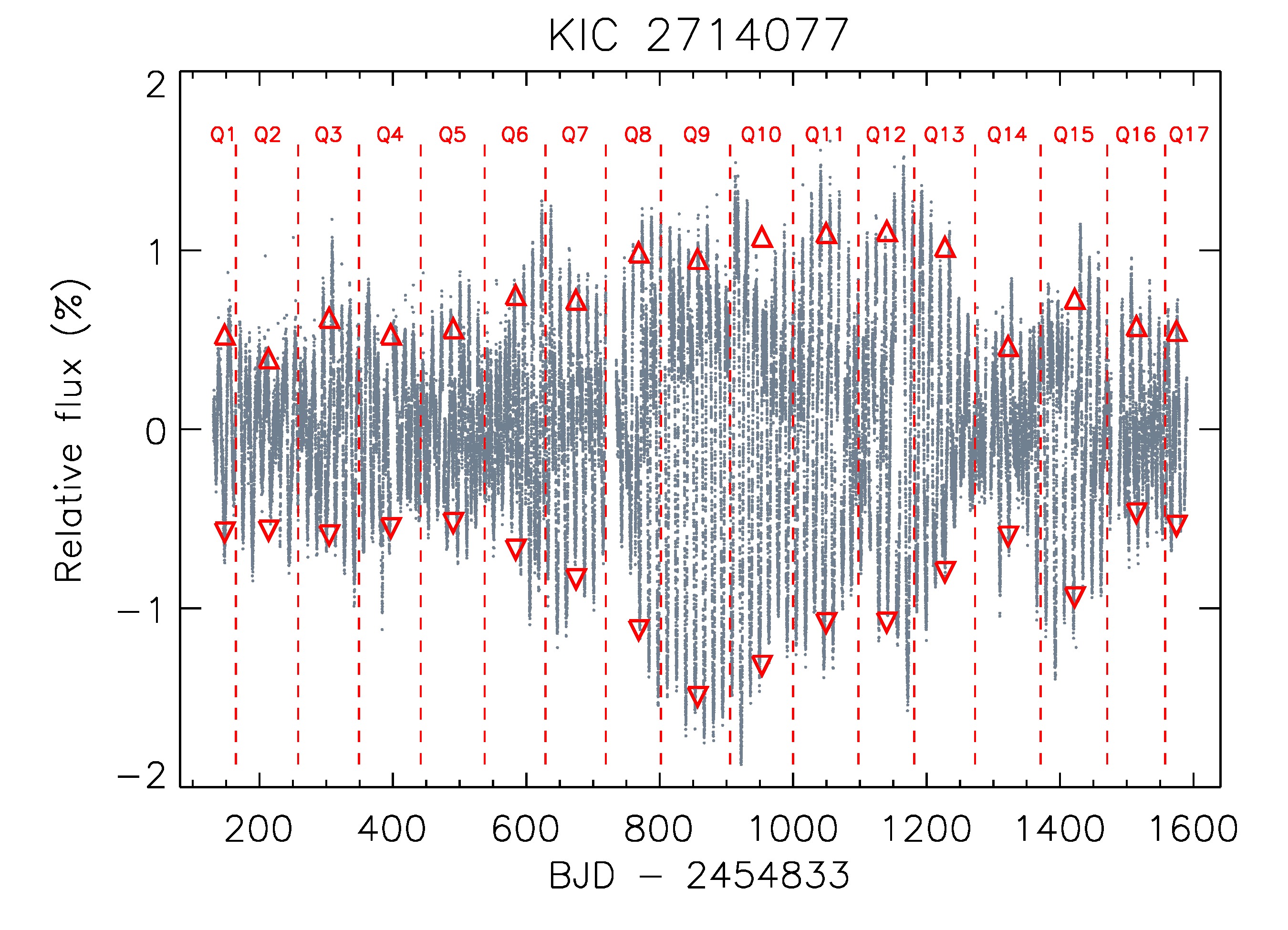 Figure 1
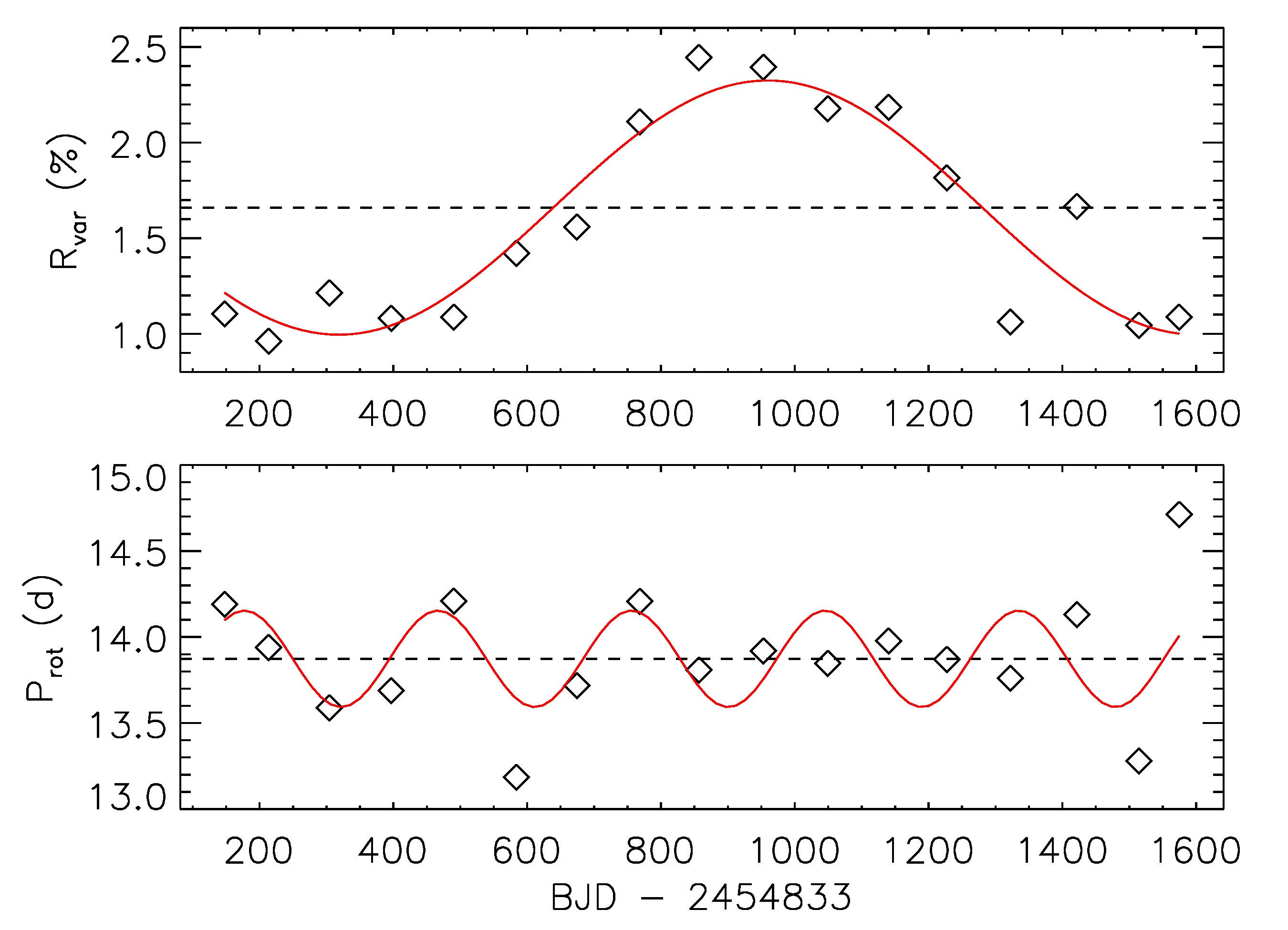 Figure 2
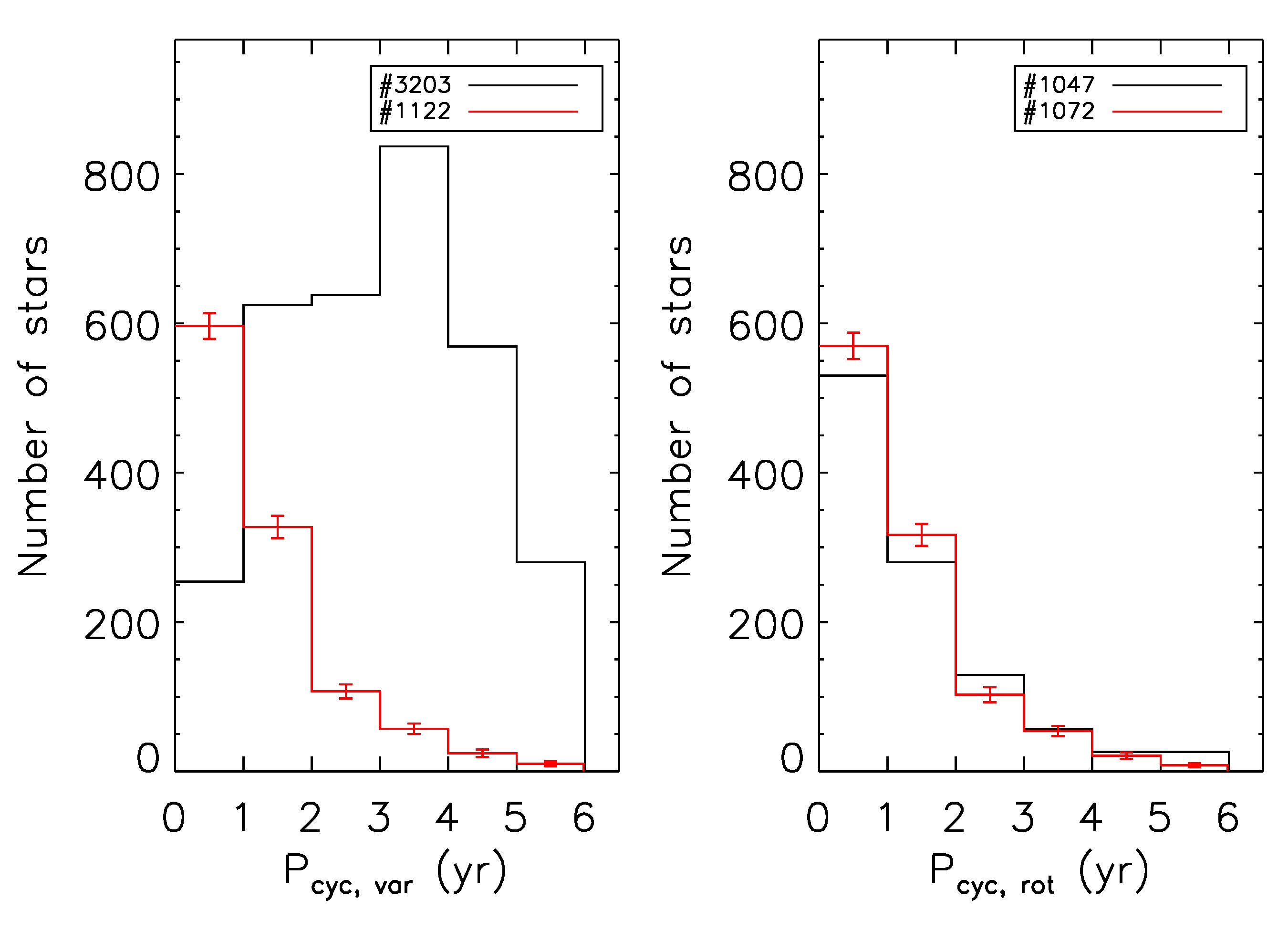 Figure 3
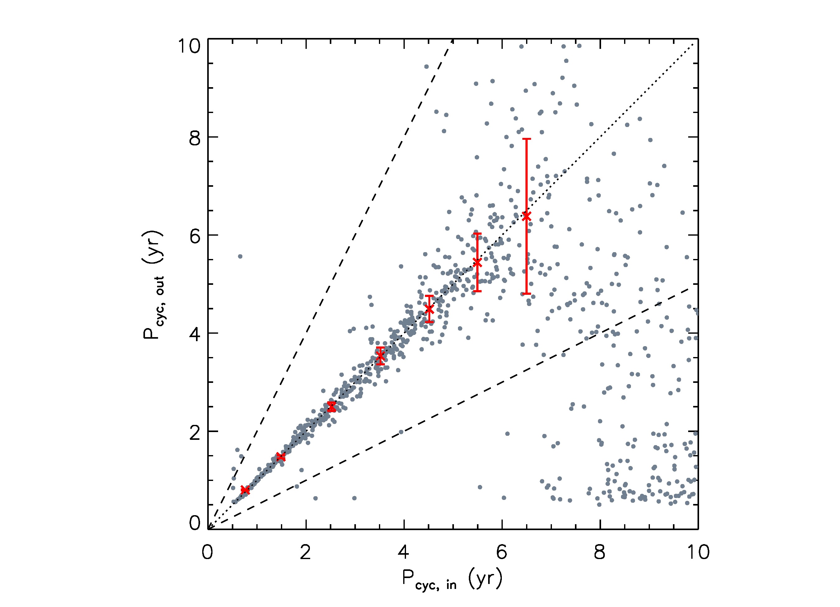 Figure 4
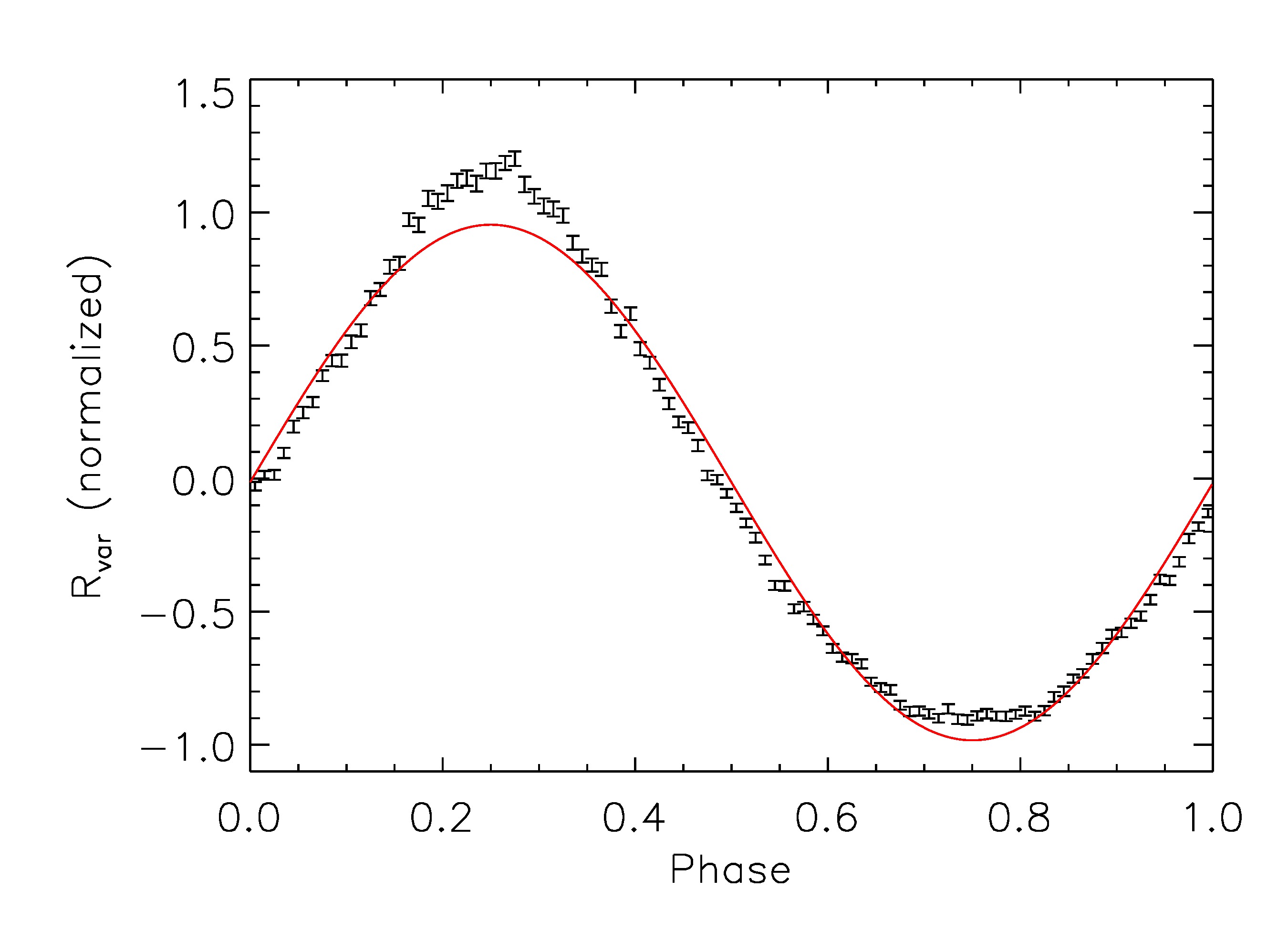 Figure 5
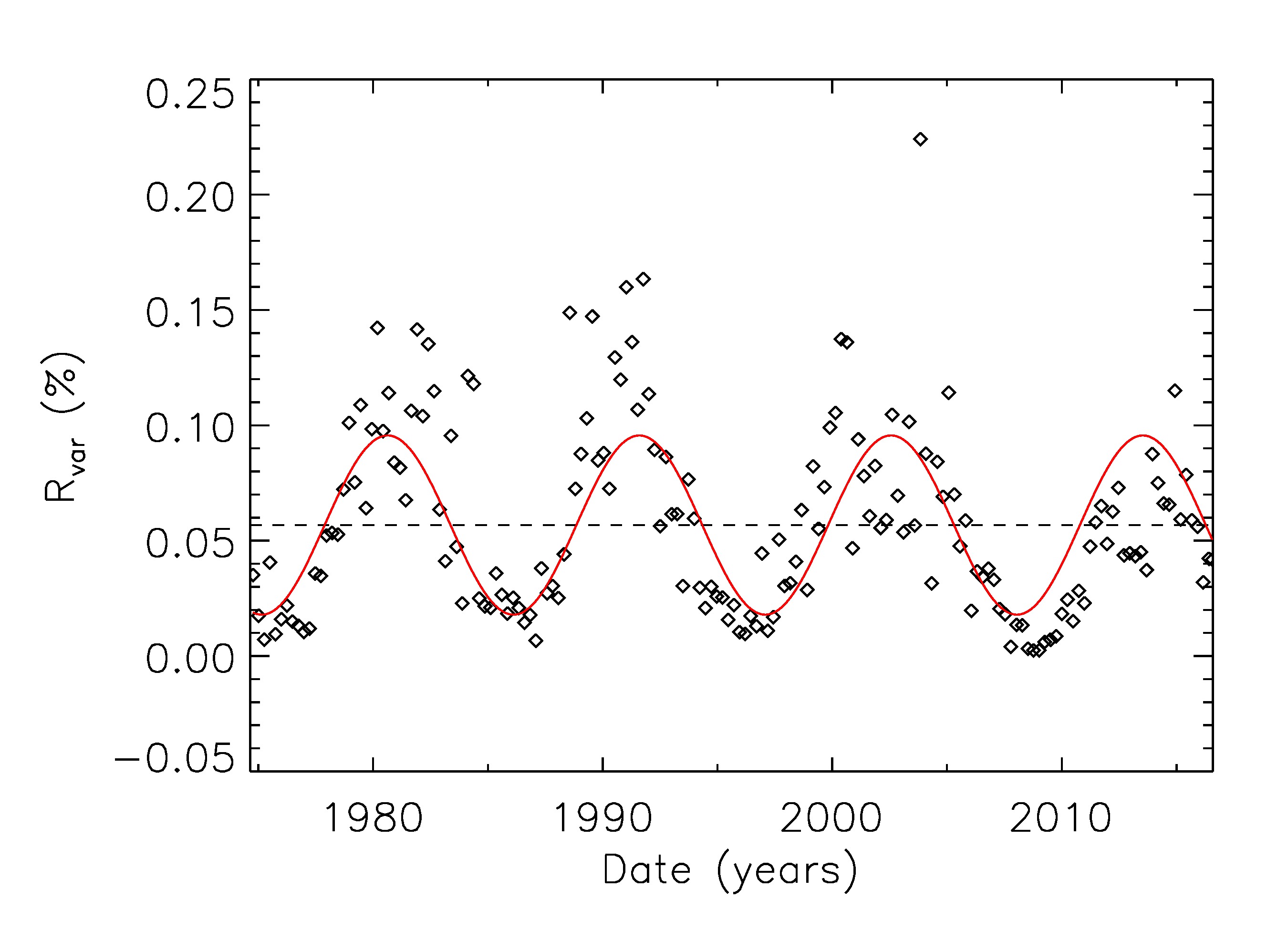 Figure 6
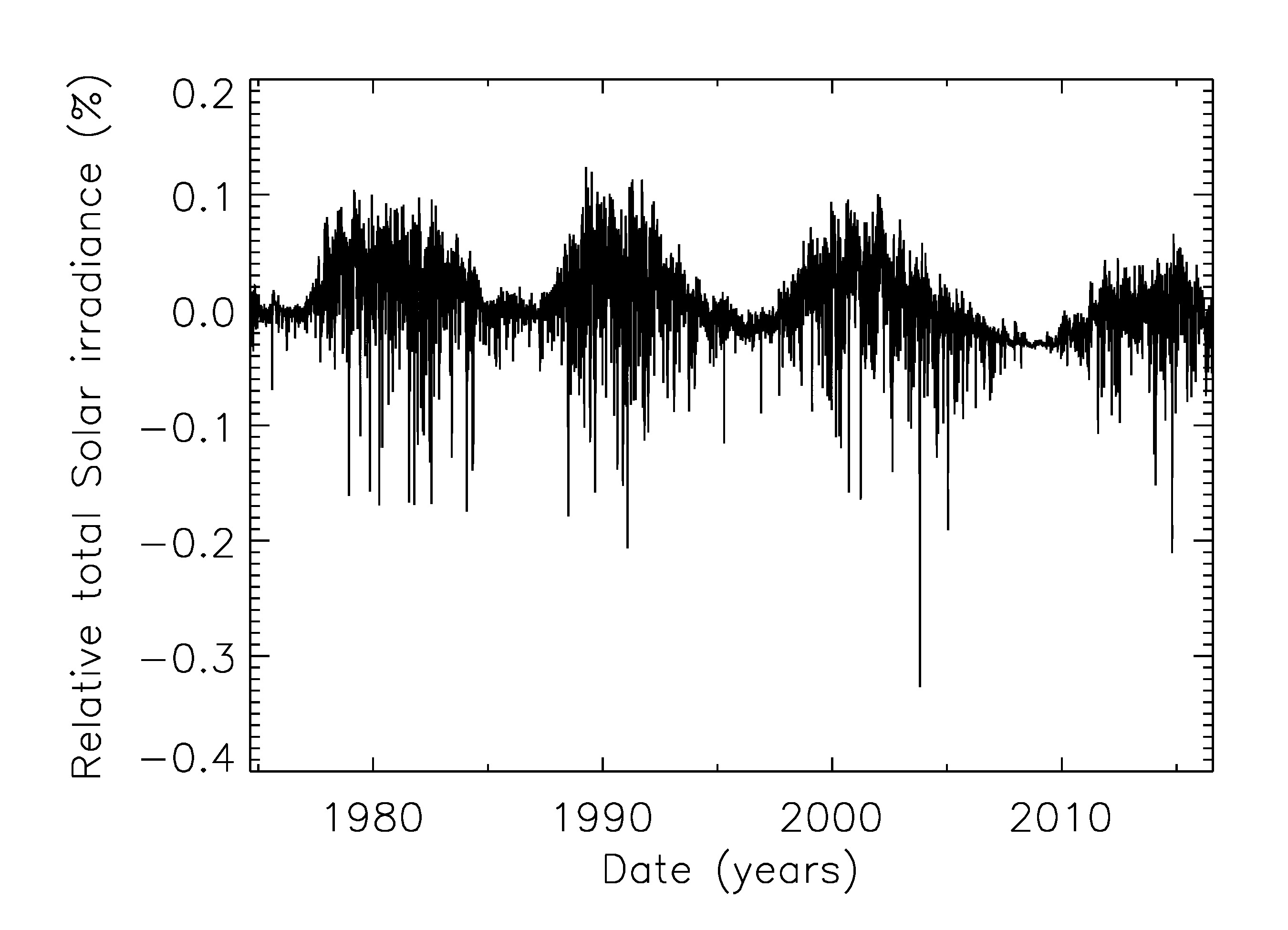 Figure 7
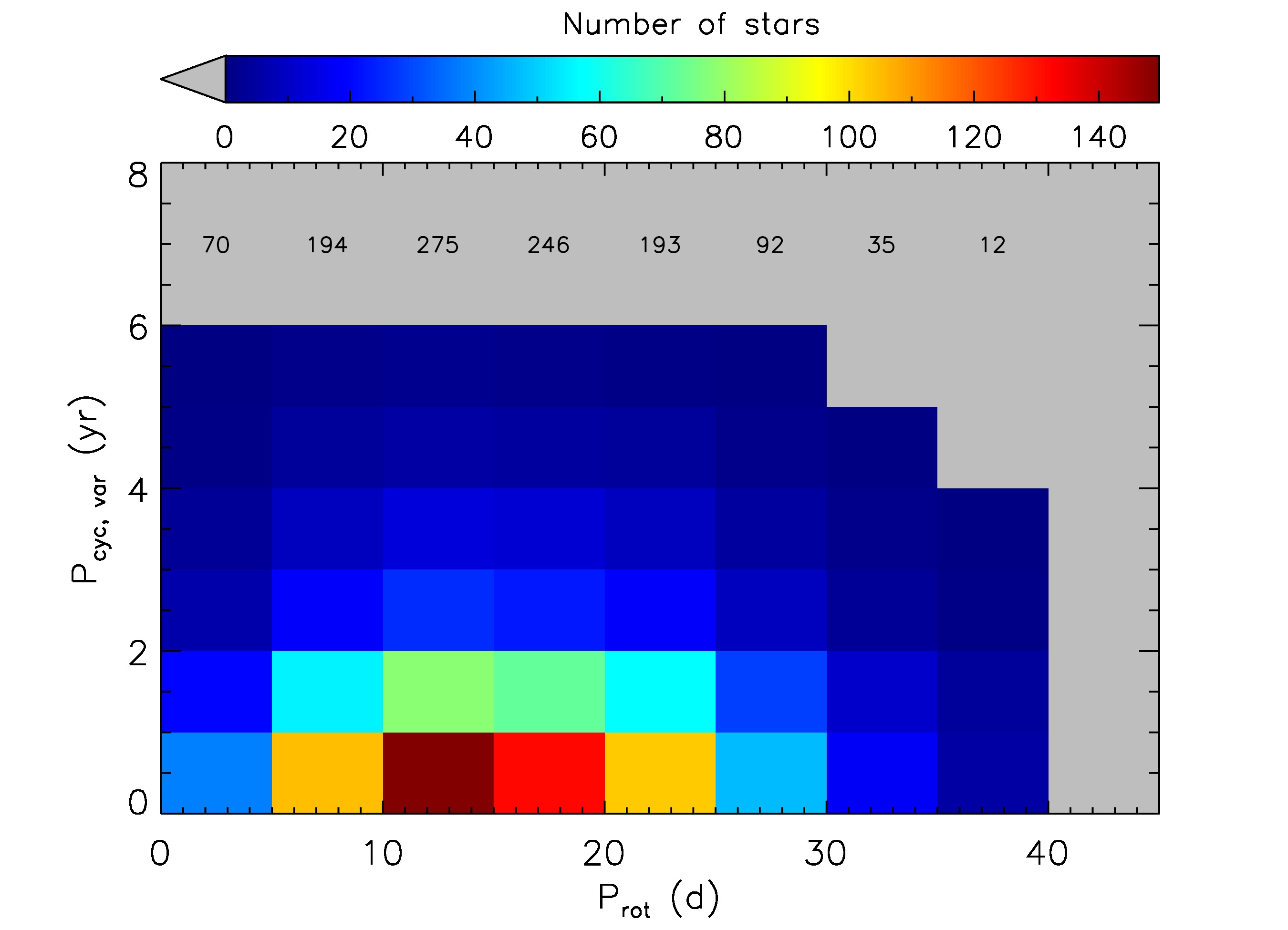 Figure 8
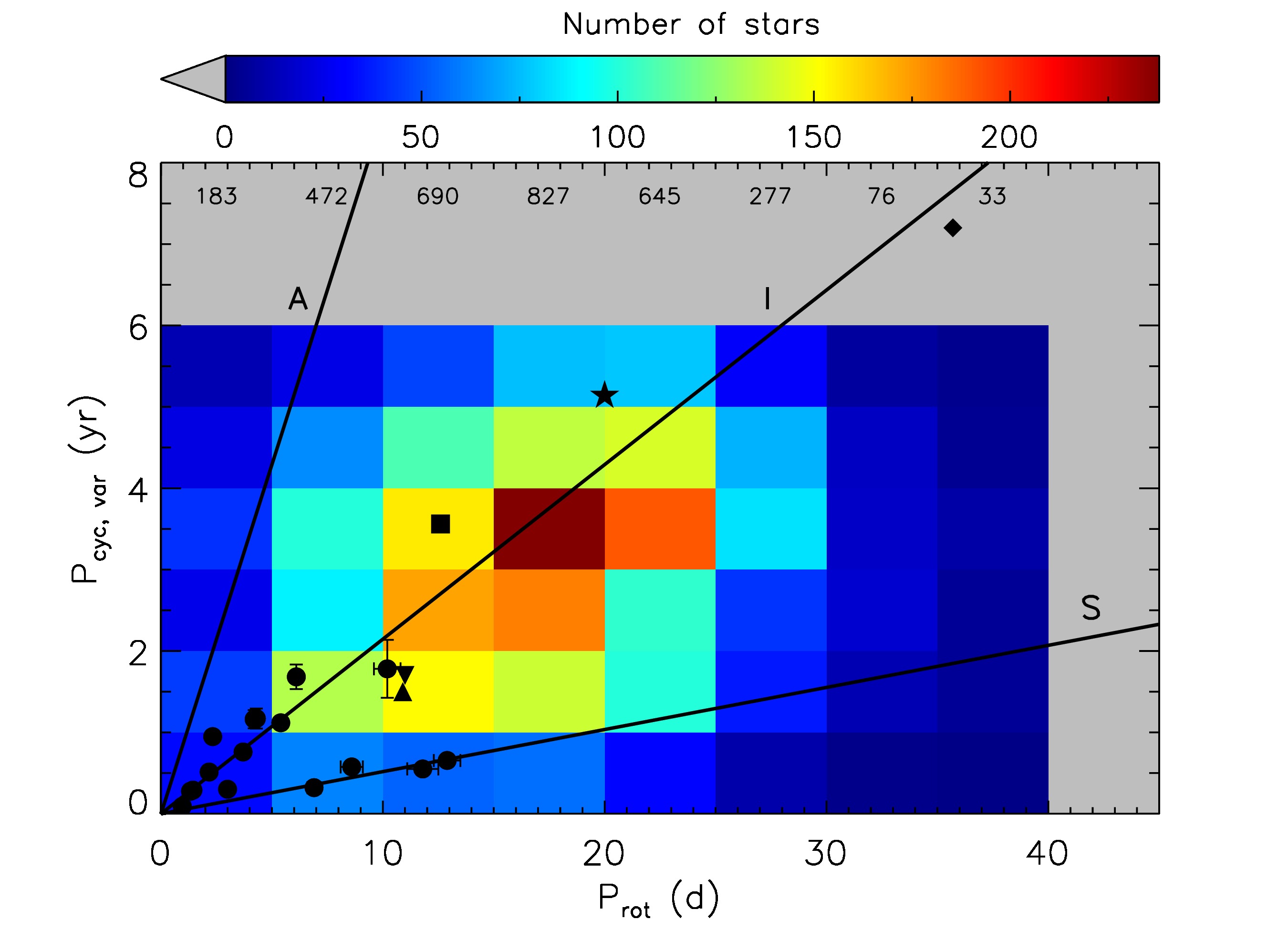 Figure 9
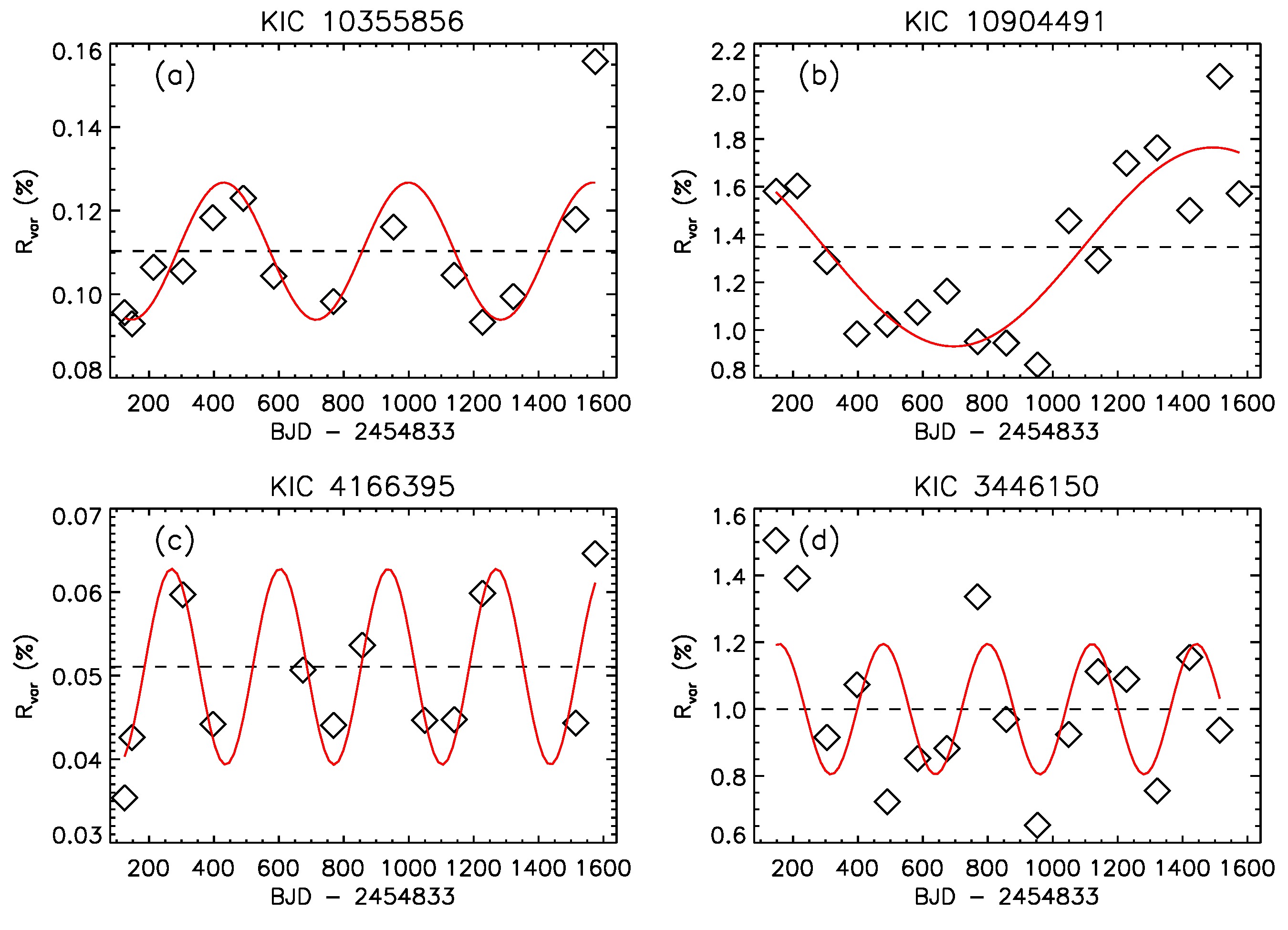 Figure 10
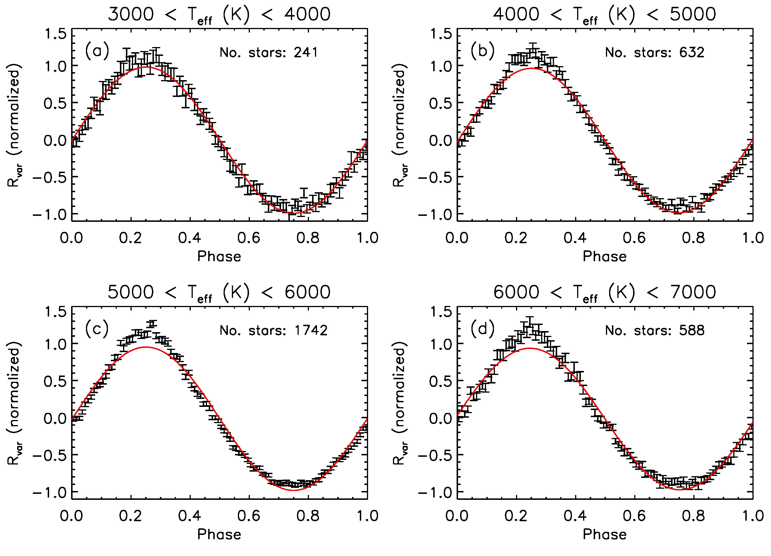 Figure 11
| (yr) | (yr) | (yr) | (%) |
|---|---|---|---|
| 0.80 | 0.01 | 1.2 | |
| 1.48 | 0.03 | 2.0 | |
| 2.50 | 0.09 | 3.6 | |
| 3.54 | 0.17 | 4.9 | |
| 4.49 | 0.27 | 6.1 | |
| 5.44 | 0.59 | 11.2 | |
| 6.38 | 1.58 | 26.2 |
Peer Reviews
No public reviews on file for this paper yet. If you reviewed it on a platform where reviews are public (OpenReview, ICLR, NeurIPS, ICML), you can paste yours below so the community can read it here.
Videos
No videos yet. Explain this paper in a talk, walkthrough, or lecture? Add one.
11institutetext: Institut für Astrophysik, Georg-August-Universität Göttingen, 37077 Göttingen, Germany 22institutetext: Max-Planck-Institut für Sonnensystemforschung, Justus-von-Liebig-Weg 3, 37077 Göttingen, Germany 33institutetext: Center for Space Science, NYUAD Institute, New York University Abu Dhabi, PO Box 129188, Abu Dhabi, UAE
Evidence for photometric activity cycles in 3203 Kepler stars
Timo Reinhold 1122
Robert H. Cameron 22
Laurent Gizon 221133 [email protected]
(Received day month year / Accepted day month year)
Abstract
*Context. *In recent years it has been claimed that the length of stellar activity cycles is determined by the stellar rotation rate. It is observed that the cycle period increases with rotation period along two distinct sequences, the so-called active and inactive sequences. In this picture the Sun occupies a solitary position in between the two sequences. Whether the Sun might undergo a transitional evolutionary stage is currently under debate.
*Aims. *Our goal is to measure cyclic variations of the stellar light curve amplitude and the rotation period using four years of Kepler data. Periodic changes of the light curve amplitude or the stellar rotation period are associated with an underlying activity cycle.
*Methods. *Using the McQuillan et al. 2014 sample we compute the rotation period and the variability amplitude for each individual Kepler quarter and search for periodic variations of both time series. To test for periodicity in each stellar time series we consider Lomb-Scargle periodograms and use a selection based on a False Alarm Probability (FAP).
*Results. *We detect amplitude periodicities in 3203 stars between years covering rotation periods between days. Given our sample size of 23,601 stars and our selection criteria that the FAP is less than 5%, this number is almost three times higher than that expected from pure noise. We do not detect periodicities in the rotation period beyond those expected from noise. Our measurements reveal that the cycle period shows a weak dependence on rotation rate, slightly increasing for longer rotation period. We further show that the shape of the variability deviates from a pure sine curve, consistent with observations of the solar cycle. The cycle shape does not show a statistically significant dependence on effective temperature.
*Conclusions. *We detect activity cycles in more than 13% of our final sample with a false alarm probability (calculated by randomly shuffling the measured 90-days variability measurements for each star) of 5%. Our measurements do not support the existence of distinct sequences in the plane, although there is some evidence for the inactive sequence for rotation periods between 5–25 days. Unfortunately, the total observing time is too short to draw sound conclusions on activity cycles with similar length as the solar cycle.
Key Words.:
Sun: activity – stars: activity – stars: starspots – stars: rotation – Techniques: photometric
††offprints: T. Reinhold,
1 Introduction
The origin of the 11-year solar activity cycle is one of the most important questions in solar and stellar physics. Over the course of one cycle the Sun undergoes phases of strong and weak activity. During the active phase of the solar cycle, dark sunspots appear on the solar surface. These spots have lifetimes of days to a few months (Petrovay & van Driel-Gesztelyi, 1997), decaying into smaller magnetic concentrations which are bright (called faculae). Individual faculae have short lives, as the magnetic flux associated with them is buffeted by turbulent convective motions, however since magnetic flux is conserved, the faculae reform and the lifetime of extended patches of faculae have much longer lifetimes. The magnetic cycle of the Sun is thus accompanied by brightness variations. This variability is weak during times of minimum activity, but the variability, being an evolving combination of dark and bright features on the rotating surface of the Sun is high during times of maximum activity. Although these activity phenomena act on different time scales they can all be detected in the total solar irradiance (TSI) data (see e.g. Domingo et al. 2009).
On stars other than the Sun cyclic activity has also been observed through (long-term) brightness changes caused by epochs of increased occurrence of active regions on the surface or in the low stellar atmosphere. The magnetic field of the active regions transports energy into the chromosphere, which leads to increased chromospheric emission, most evident in the cores of the Ca ii H&K lines. The strength of this enhancement in the emission is usually described by the so-called Mount Wilson S-index (Vaughan et al., 1978) or the related quantity (Linsky et al., 1979). A long-term study of chromospheric activity of main-sequence stars in the solar neighborhood was initiated at the Mount-Wilson observatory in the late 1960s. Wilson (1978) presented Ca ii H&K flux measurements with first evidence for cyclic variations. Vaughan & Preston (1980) found that FGKM stars exhibit different levels of chromospheric activity with a deficiency of stars of intermediate activity. These authors explained the dearth of intermediate active stars in terms of an activity decline with age. In contrast, Noyes et al. (1984a) found a tight correlation between activity and the Rossby number (defined as rotation period divided by the convective overturn time ), but could not detect evidence for the – nowadays called – Vaughan-Preston gap. Noyes et al. (1984b) detected cyclic variations of the chromospheric activity levels in 13 main-sequence stars providing the relation between the cycle period and the rotation period. Baliunas et al. (1995) investigated stars of spectral type G0-K5 and found that these can roughly be separated by their mean S-index: Fast rotators are assumed to be young objects with high S-indices, whereas older stars rotate more slowly and show lower values of the S-index, again providing evidence for the Vaughan-Preston gap. Baliunas et al. (1996) tried to understand cyclic activity in terms of stellar dynamo theory, proving a relation between the ratio of the cycle and rotation period and the dynamo number according . Brandenburg et al. (1998) and Saar & Brandenburg (1999) studied the relation between magnetic dynamo cycle period, rotation period, activity level and stellar age. These authors were the first claiming the existence of the active (A) and inactive (I) sequences, two almost parallel branches separated by a factor of six in following the relation . Additionally, for fast rotators with d these authors found evidence for a third branch with opposite slope . Böhm-Vitense (2007) confirmed that chromospherically active stars follow the A- and I-sequences in the plane. Slow rotators exhibit shorter cycle periods populating the I-sequence, whereas stars rotating faster than the Sun exhibit long cycle periods located on the A-sequence. Some A-sequence stars exhibit secondary cycle periods located on the I-branch. The Sun is located in between the two branches. In contrast, do Nascimento et al. (2015) found that the Sun does not have a solitary position between the two branches but lies on a newly proposed solar-analog sequence.
All cycle period measurements above are based on cyclic Ca ii H&K emission, but also long-term brightness variations indicate cyclic activity (see e.g. Baliunas & Vaughan 1985, nicely linking solar activity to photometric and chromospheric activity on stars other than the Sun). Oláh et al. (2000) and Oláh & Strassmeier (2002) investigated activity cycles from long-term V-band photometry. Messina & Guinan (2002) found evidence for cyclic activity in six solar-analogue stars also using long-term V-band observations. In a subsequent paper, Messina & Guinan (2003) found that also the mean rotation period changes over the course of the activity cycle. Lockwood et al. (2007) provided parallel measurements of photometric and chromospheric variability, but unfortunately did not determine any cycle periods. Oláh et al. (2009) found a positive correlation between rotational and cycle period for 20 active stars using time-frequency analysis. A similar approach was applied to Kepler light curves of very fast rotators ( d) by Vida et al. (2014). These authors found hints for cyclic activity on timescales of 300–900 days analyzing cyclic changes of the mean rotation period. Using CoRoT data Ferreira Lopes et al. (2015) detected cyclic variability in 16 FGK type stars. These authors found evidence for a possible third sequence, parallel to the previously identified active and inactive sequences, but shifted by a factor of towards shorter cycle periods. Lehtinen et al. (2016) found evidence for activity cycles in 18 solar-type stars using decades-long photometric observations. The cycle periods follow the sequences defined by Saar & Brandenburg (1999), bridging chromospherically and photometrically derived activity cycles. In recent years, activity cycles are also detected from asteroseismology through periodic shifts in the mode frequencies (García et al., 2010; Salabert et al., 2016).
The primary Kepler mission provides continuous, high-precision photometry of thousands of stars over four years of observation. Due to the presence or absence of active regions on the visible hemisphere (e.g. spots, plage) the stellar flux gradually changes. Such long-term changes are observed in the total solar irradiance data, showing significant changes over the course of the 11-year cycle. In addition, the preferred latitude of active region occurrence changes. Owing to differential rotation equatorial spots have a shorter rotation period than higher latitude spots. Our main goal is to detect cyclic changes of the light curve amplitude and the stellar rotation period, which we interpret as an indication of a photometric activity cycle. The largest sample with well determined rotation periods is provided by McQuillan et al. 2014 (hereafter McQ14). This huge sample of active stars forms the basis of our activity cycle survey.
2 Data & Method
2.1 Motivation from the Sun
As mentioned in the introduction, the brightness of the Sun (as measured by the total solar irradiance, TSI) varies due to the passage of dark sunspots and bright plage regions across the solar disk. The top panel of Fig. 1 shows the TSI time series from Shapiro et al. (2016) produced with the SATIRE-S model (Yeo et al., 2014). It is readily seen that at times of activity maxima (1979, 1989, 2000, 2014) the TSI varies rapidly, while there are only small variations during times of activity minima (1976, 1986, 1996 and 2008).
To quantify the time-dependent variability in a manner which we can easily extend to Kepler data we begin by rebinning the TSI data from a cadence of up to 1-minute to a 1-day cadence. We then break the data into 90-days segments, and following Basri et al. (2011), we define the variability range for that 90-day period as the difference between the 5th and 95th percentiles of the TSI measurements in the 90-day segment. This activity measure is similar to the magnetic index defined by Mathur et al. (2014). For each of the segments we thus obtain a measurement of the variability . Using the midpoints of each 90-days time segment we create a time series , shown in the lower panel of Fig. 1. Computing the Lomb-Scargle periodogram of the time series reveals a peak at yr, which is compatible with other estimates of the solar cycle length. This shows that this method is capable of detecting the correct cycle period from the variability of a stars light curve.
2.2 Kepler Data
Most Kepler data is released in segments of days (the so-called quarters) with exceptions for the quarters Q0 ( days), Q1 ( days), and Q17 ( days). There is an ongoing debate how to remove instrumental effects from the time series. The data studied in this paper rely on the PDC-MAP pipeline using the following versions111The version number can be found in the primary headers of the FITS files using the FILEVER keyword.: Version 2.1 for Q0-Q4 & Q9-Q11; Version 3.0 for Q5-Q8 & Q12-Q14; Version 5.0 for Q15-Q17. For each star we create a time sequence , consisting of the midpoints of the time segments covered by the quarters when a star was observed.
The upper panel of Fig. 2 shows the light curve of the Kepler star KIC 2714077. Each light curve is normalized and centered around zero by dividing the flux by its median value and subtracting unity. This normalization is necessary because the Kepler spacecraft rolls between consecutive quarters, so the stars fall on different CCDs accompanied by offsets of the PDC-MAP flux between the quarters. Because the stellar variability we are interested in is that due to the rotation of spots and faculae across the disk, we further fit and subtract a second order polynomial from the data in each quarter. This will substantially reduce the influence of possible longer term instrumental issues while only slightly affecting modulation comparable or faster than the rotation period of the star. We then use the defined in the same way as for the Sun as a measure of the variability. The red triangles in the upper panel of Fig. 2 indicate the 5th and 95th percentiles of the relative flux in each quarter. The difference between the 5th and 95th percentiles equals , which is shown as time series in the middle panel of Fig. 2. The time series shows strong periodicity with a period of yr, shown as red sine fit to the data.
In addition, to measuring , for each star we also measure the stellar rotation period in each quarter using the Lomb-Scargle periodogram resulting in a time series , which is shown for the same stars in the lower panel of Fig. 2. The quarterly measured rotation periods scatter around the mean rotation period d. In contrast to the time series does not show strong periodicity. The Lomb-Scargle periodogram finds a peak at a period less than one year, which is visualized by the red sine fit to the data. As we will show in the following, strong periodicity of the variability range and random scatter of the rotation period time series is quite common for many stars of our sample.
Owing to the limited quarter length we set upper limits on the detectable rotation periods: 10 days for Q0, 30 days for Q1 & Q17, and 45 days for the other quarters. All period measurements deviating by more than 30% from the median period of all quarters were discarded. Also the measurements of these quarters were discarded because instrumental artifacts might dominate the photometry. To achieve meaningful variability and rotation period time series we require measurements in at least quarters. These conditions shrinks the initial McQ14 sample to stars. We suspect that there might be more candidates with detectable activity cycle that were missed due to our constraints so far.
2.3 Analysis of the time series
For each star we have 3 time series, , and of length , which is the number of quarters where a rotation period could be measured. The Lomb-Scargle periodogram is a straightforward way to look for periodicities in unevenly sampled data. We compute the Lomb-Scargle periodogram of the time series and (using the time series ) to test for periodicity. We call these periods associated with the highest peaks in the Lomb-Scargle periodograms and , respectively.
Because we are simply taking the highest peak in the Lomb-Scargle periodogram, and will be defined for every star. To define a subset of the stars where the inferred periodicity is more likely to be real, we introduce a False Alarm Probability (hereafter FAP) threshold. We calculate the FAP by considering 1000 random permutations of and . For each permutation we have three time series , and . We then create Lomb-Scargle periodograms for these new sequences and again concentrate on the highest peaks. We define the FAP for to be the number of cases where a higher peak appears in the Lomb-Scargle periodogram of than the one which was found for divided by the number of permutations considered.
We define the so-called periodic sample by selecting those stars for which the FAP was less then 5%. The samples are defined independently for and . The time series of three representative stars from the periodic sample are shown in panel (a)-(c) in Fig. 3. For comparison panel (d) shows a star with . We discuss the issue of false positives in the results section.
2.4 Method sensitivity
To test the sensitivity of the method to different cycle periods, we created a set of synthetic time series . We randomly selected data points, , from the time series . The time series are pure sine functions with input periods uniformly distributed between . The amplitudes are uniformly distributed random numbers, comparable to the sine fit amplitudes of the periodic sample. We add noise to the time series , which we define as standard deviation of the difference between and the best sine fit from the periodic sample. The noise distribution is Gaussian. Because the quantity describes a relative flux difference, the sine amplitude and the noise are linearly correlated. For simplicity, the phase and the offset of the sine curves are set to zero. We analyze the set of synthetic light curves using the Lomb-Scargle periodogram, and compare the returned cycle periods to the input periods in Fig. 4. This Monte-Carlo test reveals that we can trust cycle periods up to six years.
In the same way the uncertainties of the derived cycle periods have been estimated. For different cycle period bins between 0.5–10 years we created a set of synthetic light curves for each bin, and applied the above analysis. In Fig. 4 the red crosses show the median value of and the error bars show the median absolute difference between and . We omit error bars for yr because the uncertainties become huge. The associated periods and uncertainties up to yr are given in Table 1.
3 Results
3.1 Cycle periods
The cycle period distribution of for all stars satisfying is shown in black in the left panel of Fig. 5, and the distribution of for all stars satisfying is shown in black in the right panel of Fig. 5.
Assuming the time series and do not contain any periodic signal, one would obtain a number of 1180 stars after applying a limit of to a total sample of 23,601 stars. For the cycle periods of the variability amplitude we detect 3203 cycles. This number is significantly higher than the expected number of false-positive detections.
To test whether the different number of detections might be an artifact of the method we performed a Monte-Carlo simulation where we replaced the time series of each star with a random permutation of that star’s time series. We then applied exactly the same analysis as was applied to the original time series (see Sect. 2.3).
This randomization process is repeated 500 times for the whole sample. Comparing the peak height of the initially randomized time series to the peak heights of the remaining ones yields the false alarm probability for each star. We repeated this process 500 times, and found that on average 1122 stars satisfied our selection criteria. This is consistent with the expectation from the condition applied to 23,601 stars.
The averaged cycle period distribution from the Monte-Carlo experiment is shown in red in Fig. 5, with error bars showing the standard deviation of different realizations. It is obvious that the distributions of of the original and the randomized data are very different. The distribution of the real data has a maximum around three years, whereas the randomized sample mostly contains short cycles between one and two years.
In the right panel the distribution of reveals a completely different picture. The distributions of the real data and the randomized sample are largely consistent, and the total number of detections is almost identical. This shows that we cannot distinguish whether a cyclic change of the rotation period might indicate an activity cycle or if this change occurs just by chance. We conclude that we cannot use the quantity to search for activity cycles. Thus, we concentrate on in the following.
Fig. 6 shows the dependence of on the stellar rotation period for all 3203 stars of the periodic sample. The number of stars in each bin on the abscissa is given in black above the color bins.
We turn now to the issue of the cycle period’s dependence on rotation period. Our observations only allow activity periods of less than six years to be detected. From Fig. 6 it is obvious that most cycle periods have a length between 2–4 years (compare Fig. 5), slightly clumping at rotation periods between 10–20 days. Up to rotation periods of 25 days the cycle period slightly increases with rotation period. For stars rotating even slower the cycle period behavior is hard to tell from the data. Using unit weights for all data points a linear fit yields yr, i.e. a weak dependence of the cycle on rotation period. This result is confirmed by the small Pearson correlation coefficient between the two quantities.
Some previous authors have reported a correlation between the rotation period of a star and the period of its activity cycle, with periods preferentially lying on active and inactive branches (shown in Fig. 6), and with some stars having detectable periodicities of their activity cycles lying on both branches. Clearly our detection scheme can not find multiple activity periodicities, and we find that most of our detections are concentrated along the inactive branch, however the distributions are broad.
For comparison photometric cycle measurements of 16 CoRoT stars (Ferreira Lopes et al., 2015) are shown as black circles in Fig. 6. The upside down triangle, normal triangle, square, star, and diamond show measurements from Egeland et al. 2015; Salabert et al. 2016; Moutou et al. 2016; Flores et al. 2016; Boro Saikia et al. 2016, respectively. Egeland et al. (2015) also detected a longer activity cycle of yr for the same star (HD 30495).
To check that Fig. 6 is not due to a hidden selection bias, we made the same figure beginning from the Monte-Carlo simulations discussed above. The result is shown in Fig. 7. As expected from pure noise most cycle period detections lie in the range of 1–2 years because the periodogram interprets the noise as short cycles. Furthermore, the sample shows a flat distribution, i.e., no dependence on rotation. The associated Pearson correlation coefficient equals , on average, showing that and are uncorrelated.
3.2 Cycle shapes
So far we focused on the cycle periods but have not considered the shape of the variability. Fig. 8 shows a phase-folded curve of the variability range averaged over all stars of the periodic sample. All time series are phase-folded with the measured cycle period and shifted that they all lie in phase. The mean variability level is subtracted, and the curves are normalized by their amplitudes. The average over all curves is shown in black and the red curve shows a sine fit. The error bars show the standard error in each phase bin. It is clear that the shape of the variability shows some deviation from a pure sine curve. At maximum activity the observed variability curve is more spiky than a sine curve. At minimum activity the variability is rather flat. Applying the same analysis to the time series of the TSI data (compare Fig. 1) we also find a flat shape at minimum activity, but a large scatter at maximum activity. To quantify the deviation of the data from the sine curve we compute the reduced chi-square and the associated p-value to be and , respectively, indicating a high statistical significance for the deviation from a sinusoidal shape.
Fig. 9 shows the same curve as Fig. 8 for different temperature bins. In each bin the stars have roughly the same cycle period distribution. The coolest stars are well represented by a sine curve. Neither the spiky top nor the flat bottom are visible. The shape of the curve gradually changes towards hotter stars. The top becomes more spiky and the bottom flattens out. To quantify the temperature dependence we calculate the difference between each of the six possible pairs of the average curves (a)–(d) in Fig. 9. We do not find a statistically significant difference between the pairs that would indicate a temperature dependence of the cycle period. The slightly different cycle shape in panel (a) might be explained by the smaller number of stars in this temperature bin.
4 Summary
We detected periodicity of the variability amplitude in 3203 stars of the McQ14 sample, which we interpreted as indication for an underlying activity cycle. To account for random detections, the original sample was compared to a randomized sample. It was found that the number of activity cycle detections was three times higher than expected from pure noise. We did not detect cycles changes of the rotation period beyond those expected from noise. The plane revealed that the cycle period shows weak dependence on the rotation period, slightly increasing with rotation period. In contrast to previous studies (Noyes et al., 1984b; Baliunas et al., 1996; Saar & Brandenburg, 1999; Böhm-Vitense, 2007; Ferreira Lopes et al., 2015; Lehtinen et al., 2016) we did not find evidence for a tight functional dependence between the cycle and the rotation period. Our measurements show a large scatter around the inactive branch. Previous studies (Saar & Brandenburg 1999; Böhm-Vitense 2007) have shown stars with multiple periodicities on the A- and I-branches. These studies were based on chromospheric activity indices, which will have different sensitivities to spots and plage than the photospheric variability detected using Kepler data. Hence it is possible that our finding of a strong I-branch and little evidence of the A- and S-branches might indicate that the I-branch has a stronger signature in the photosphere than the A- or S-branches. In good agreement with the solar cycle the average shape of all activity cycles was found to deviate from a pure sine curve. We could not detect a statistically significant temperature dependence of the activity cycle shape.
Acknowledgements.
The research leading to these results received funding from EU FP7 collaborative project “Exploitation of space data for innovative helio- and asteroseismology” (SpaceInn) under grant agreement No. 312844. L.G. acknowledges support from the NYU Abu Dhabi Institute under grant G1502. This work was supported in part by the German space agency (Deutsches Zentrum für Luft- und Raumfahrt) under PLATO grant 50OO1501. Part of the research leading to the presented results has received funding from the European Research Council under the European Community’s Seventh Framework Programme (FP7/2007-2013) / ERC grant agreement no 338251 (StellarAges).
The reference list from the paper itself. Each links out to its DOI / PubMed record.
- 1Baliunas et al. (1995) Baliunas, S. L., Donahue, R. A., Soon, W. H., et al. 1995, Ap J, 438, 269
- 2Baliunas et al. (1996) Baliunas, S. L., Nesme-Ribes, E., Sokoloff, D., & Soon, W. H. 1996, Ap J, 460, 848
- 3Baliunas & Vaughan (1985) Baliunas, S. L. & Vaughan, A. H. 1985, ARA&A, 23, 379
- 4Basri et al. (2011) Basri, G., Walkowicz, L. M., Batalha, N., et al. 2011, AJ, 141, 20
- 5Böhm-Vitense (2007) Böhm-Vitense, E. 2007, Ap J, 657, 486
- 6Boro Saikia et al. (2016) Boro Saikia, S., Jeffers, S. V., Morin, J., et al. 2016, A&A, 594, A 29
- 7Brandenburg et al. (1998) Brandenburg, A., Saar, S. H., & Turpin, C. R. 1998, Ap J, 498, L 51
- 8do Nascimento et al. (2015) do Nascimento, Jr., J.-D., Saar, S. H., & Anthony, F. 2015, in Cambridge Workshop on Cool Stars, Stellar Systems, and the Sun, Vol. 18, 18th Cambridge Workshop on Cool Stars, Stellar Systems, and the Sun, ed. G. T. van Belle & H. C. Harris, 59–64