
TL;DR
This paper introduces a novel three-dimensional random point field based on quaternion determinants, providing explicit formulas and asymptotic analysis of the kernel and orthogonal polynomials in the bulk and at the center.
Contribution
It develops a new 3D Ginibre point field using quaternion determinants, with explicit formulas and asymptotic behavior analysis.
Findings
Explicit formulas for polynomials and kernels
Asymptotic behavior in bulk and at the center
Extension of Ginibre ensemble to 3D using quaternions
Abstract
We introduce a three-dimensional random point field using the concept of the quaternion determinant. Orthogonal polynomials on the space of pure quaternions are defined, and used to construct a kernel function similar to the Ginibre kernel. We find explicit formulas for the polynomials and the kernel, and calculate their asymptotics in the bulk and at the center of coordinates.
Click any figure to enlarge with its caption.
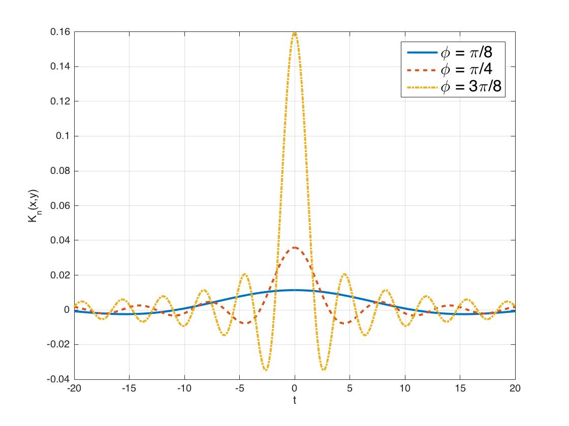 Figure 1
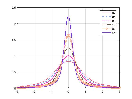 Figure 2
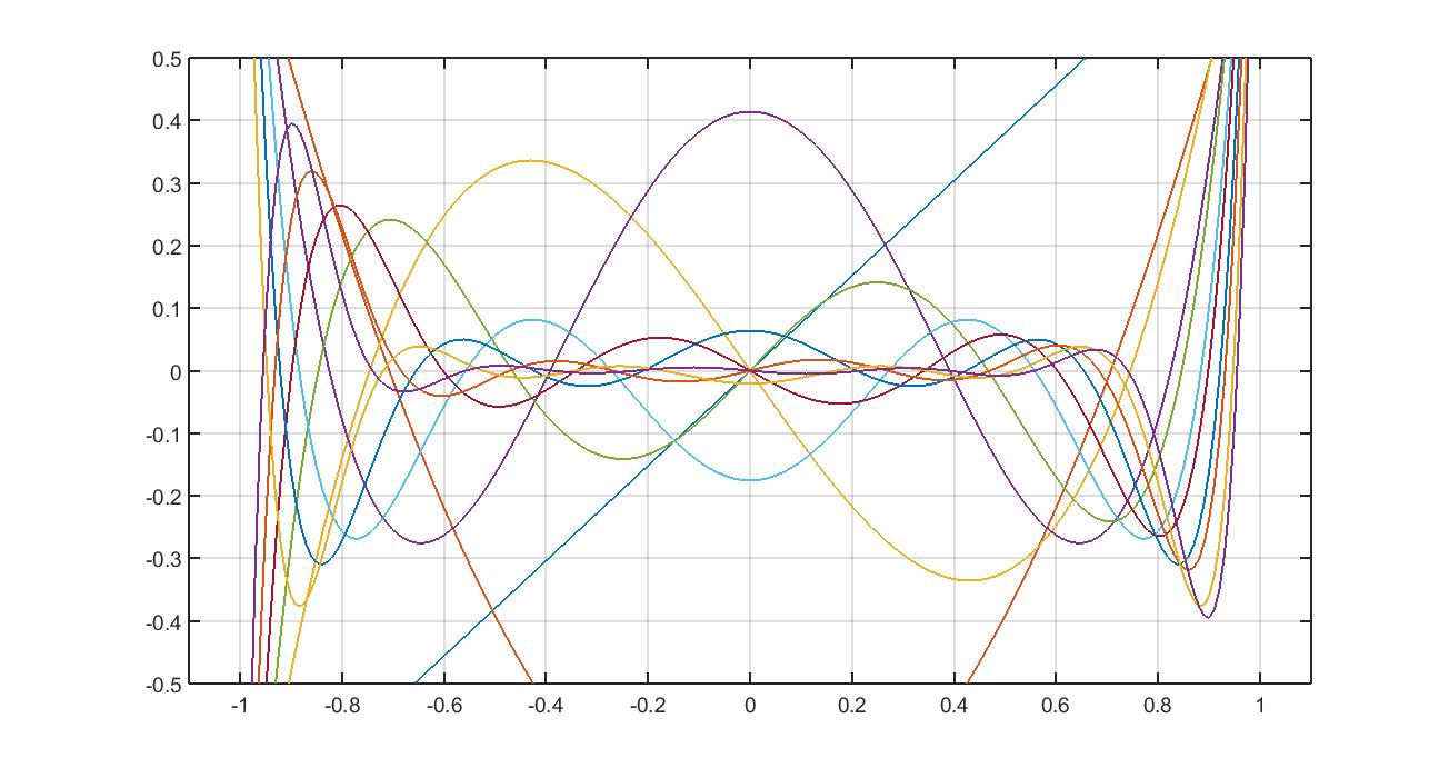 Figure 3
| m/n | 0 | 1 | 2 | 3 | 4 | 5 | 6 |
|---|---|---|---|---|---|---|---|
| 0 | 1 | 0 | 0 | 0 | |||
| 1 | 0 | 0 | 0 | 0 | |||
| 2 | 0 | 0 | 0 | ||||
| 3 | 0 | 0 | 0 | 0 | |||
| 4 | 0 | 0 | 0 | ||||
| 5 | 0 | 0 | 0 | 0 | |||
| 6 | 0 | 0 | 0 |
| 0 | 1 | 1 | * |
| 1 | 3 | 3 | |
| 2 | 6 | 2 | |
| 3 | 30 | 5 | |
| 4 | 120 | 4 | |
| 5 | 840 | 7 | |
| 6 | 5,040 | 6 | |
| 7 | 45,360 | 9 | |
| 8 | 362,880 | 8 | |
| 9 | 3,991,680 | 11 |
| 0 | 1 |
|---|---|
| 1 | |
| 2 | |
| 3 | |
| 4 | |
| 5 | |
| 6 | |
| 7 | |
| 8 | |
| 9 |
Peer Reviews
No public reviews on file for this paper yet. If you reviewed it on a platform where reviews are public (OpenReview, ICLR, NeurIPS, ICML), you can paste yours below so the community can read it here.
Videos
No videos yet. Explain this paper in a talk, walkthrough, or lecture? Add one.
A 3D Ginibre point field
Vladislav Kargin111email: [email protected]; current address: Department of Mathematics, Binghamton University, Binghamton, 13902-6000, USA
We introduce a three-dimensional random point field using the concept of the quaternion determinant. Orthogonal polynomials on the space of pure quaternions are defined, and used to construct a kernel function similar to the Ginibre kernel. We find explicit formulas for the polynomials and the kernel, and calculate their asymptotics in the bulk and at the center of coordinates.
Contents
1. Introduction
Informally, a random point field is a configuration of points in a space selected according to a joint probability distribution. If the joint distribution can be written as a product of marginal distributions for different points, then the points are “independent” or not “interacting”, so that their locations are independent from each other. However, there are many interesting point fields, in which points are not independent.
An important class of such dependent point fields are determinantal fields, in which the joint distribution can be written as a determinant of a kernel function (see Dyson ([4]), Macchi ([11], Mehta ([12]), Soshnikov ([13], Hough et al. ([7])).
In particular, the eigenvalues of non-Hermitian Gaussian random matrices form a determinantal field in the complex plane ([6]) with an interesting complex-valued kernel,
[TABLE]
This random point field is called the Ginibre ensemble. It is quite remarkable since its kernel is among the small number of kernels which are invariant relative to a large group of complex plane transformations. (See Krishnapur [10] ).
The Ginibre kernel is quite natural in the sense that polynomials are orthonormal with respect to the standard Gaussian measure in the plane. In particular, this kernel can be considered as the kernel of the orthogonal projection from the space of all polynomials on to the - dimensional space of complex valued polynomials of degree no larger than .
Our goal in this paper is to develop a parallel theory for a similar quaternion-valued kernel,
[TABLE]
Here and are purely imaginary quaternions, which we identify with points in , and polynomials are the monic quaternion polynomials of degree , which are orthogonal with respect to the standard Gaussian measure on .
More precisely, let We identify elements or with pure quaternions, that is, with elements of that have no real component, .
As the background measure on , we take
[TABLE]
where is the Lebesgue measure on and
[TABLE]
(In particular, )
Next, let be the right -module of polynomial functions on the space of imaginary quaternions . Elements of this module are defined as finite sums of where are arbitrary quaternions and ,
[TABLE]
Let a scalar product on this space be defined by
[TABLE]
This function is linear in the second argument
[TABLE]
for every , and it also has the property that .
In addition, the scalar product is positive definite:
[TABLE]
and equality holds only if
We say that a family of quaternionic functions on is orthonormal, if
[TABLE]
Let denote the system of monic orthogonal polynomials. We can show that this system exists and unique by the Gram-Schmidt orthogonalization process.
It turns out that , and we will study these polynomials in detail. The constants in formula (1) ensure that polynomials have unit norm.
The rest of the paper is organized as follows. In Section 2 we give an overview of main results. In Section 3 we briefly review the theory of quaternion determinantal fields. In Section 4 we study the orthogonal polynomials and the norm constants . Section 5 is devoted to the study of properties of the kernel. And Section 6 concludes with open problems.
2. Brief description of the results
For the monic orthogonal polynomials we obtain a formula that relates them to Hermite polynomials and calculate the norm of .
{restatable*}
theotheoHermite
Let pure quaternion , where and . Then
[TABLE]
(The numbering of theorems refers to the section where they are proved. For example, this theorem is restated and proved in Section 4.)
The norms of these polynomials are given by the following formula,
[TABLE]
The kernel is defined by formula (1), and it turns out that an analogue of the Christoffel-Darboux formula holds.
{restatable*}
theotheoKernelFormula
Let and , where and . Suppose . Then
[TABLE]
where
[TABLE]
Here the and determined by the following condition. If is a unit pure quaternion, then
[TABLE]
Next, define
[TABLE]
{restatable*}
theotheoDensity
Let denote the density of the random field at point with respect to the Lebesque measure on . Assume that is a pure unit quaternion and , . Then,
[TABLE]
Intuitively the theorem says that (i) with high probability a random field point is contained in the ball of radius ; (ii) the average density of points in the ball is , and (iii) after rescaling the density has the form given by the function .
Next, let us define the radial density
[TABLE]
where is the sphere of radius and is the measure on induced by the Lebesgue measure on . The radial density summarizes how the points are distributed over the different spherical shells. Inside each shell, the distribution is rotationally invariant.
{restatable*}
corocoroRadialDensity
We have
[TABLE]
Next, we check that if and are fixed and different, then the limit of the expression for is [math] for . There are no 2-correlations at this scale.
In order to understand what happens when is sufficiently close to , we consider the case, in which . We will correct it a bit since the scaling depends on the density of the field, and the density varies with .
Let
[TABLE]
Define
[TABLE]
where and are real parameters. (We use factor for the convenience of calculations in the proof. The factor works equally well.) Note that is of the order .
It will be convenient to use the notation
[TABLE]
where and are pure unit quaternions, and are real, , and is as defined in (6).
{restatable*}
theotheoBulkAsymptotic
Let and , the space of pure unit quaternions. Then,
[TABLE]
This gives us a kernel on the space as a scaling limit of the quaternion kernels on .
At the center the situation is different.
{restatable*}
theotheoKernelCenter
Let and , where and . Suppose . Then
[TABLE]
In the next section we begin a more detailed discussion of these results.
3. Definition of the determinantal point field
3.1. Existence results
Let and the background measure be a Radon measure on (that is, a Borel measure which is finite on compact sets).
Definition 3.1**.**
A random point field on is a random integer-valued positive Radon measure on .
For a set , we can interpret as the number of points in (counted with multiplicities, perhaps). We will assume our fields to be simple, so that each point has a multiplicity at most .
A random point field can be described by its correlation functions.
Definition 3.2**.**
A locally integrable function : is called a -point correlation function of a random point field if for any disjoint measurable subsets of and any non-negative integers such that the following formula holds:
[TABLE]
where denote expectation with respect to random measure .
If we set all and let to be infinitesimally small, then we can see that is the density of the probability to find a point in a neighborhood of each of the points .
More generally, left hand side can be interpreted as a joint ordered moment of the number of points in sets
A random point field is traditionally called determinantal if all of its correlation functions can be represented as determinants:
[TABLE]
where is a kernel function that maps to . We extend this definition to include the case of quaternion determinants.
Definition 3.3**.**
A random point field on is determinantal if its correlation functions are given by the formula:
[TABLE]
where maps to , the skew field of (real) quaternions, and is the Dyson-Moore determinant.
For the case when kernel takes values in , this definition agrees with definition in (12). For quaternion kernels this definition only makes sense if the kernel is self-dual, that is, . (See [2], [15], and [5] for more information about quaternion matrices and their determinants.)
A basic question is “Which kernels lead to a valid collection of correlation functions?” One sufficient condition is as follows.
\egothfamilySatz 3.4 (Dyson-Mehta).
Suppose that the kernel can be written as
[TABLE]
where is an orthonormal system of quaternion functions on . Then there exists a random point field on with the correlations given by (13), and the total number of points is almost surely equals
This result was essentially proved by Dyson ([4]) and generalized by Mehta ([12], Theorem 5.1.4).
By Theorem 3.4 the kernel
[TABLE]
defines a valid determinantal field provided that are orthonormal polynomials with respect to the measure .
The next section is devoted to the existence and properties of these polynomials. Then we will study the properties of the kernel.
4. Orthogonal polynomials
4.1. Scalar Product
We look for the orthonormal basis of the space of polynomials with respect to the scalar product
[TABLE]
We can find this basis by applying the Gram-Schmidt procedure to the monomial basis For this purpose we compute the scalar products of monomials.
\egothfamilySatz 4.1.
For all non-negative integers and
[TABLE]
The proof of this result can be found in Appendix B.
Since all entries in the matrix of scalar products are real, we derive an important consequence that the coefficients of monic orthogonal polynomials are real.
Note that , which means that the scalar product cannot be written as for a measure on the real line.
4.2. Three-term recurrence relation
By usual means, we can derive the three-term recurrence relation for the orthogonal polynomials.
\egothfamilySatz 4.2.
Suppose that are monic polynomials orthogonal with respect to the scalar product in (14), and that and . Then these polynomials satisfy the following recurrence relation:
[TABLE]
where are some real positive coefficients, and
[TABLE]
Proof: Let us start with the expression
[TABLE]
Then for all We also calculate that
[TABLE]
if we take
[TABLE]
Similarly,
[TABLE]
if we take
[TABLE]
With this choice of and polynomial has degree and orthogonal to for all . Since polynomials form a basis, hence . By using the definition of the scalar product (14) we conclude that Hence
[TABLE]
By induction it is easy to see that all are odd polynomials, all are even, and thereforre for all . In addition, it is easy to see that all are real.
To conclude, we need to modify formula (16) for . By using property and the fact that the coefficients of orthogonal polynomials are real, we see that .
Since , we compute , and therefore, . This concludes the proof of the proposition.
Table 2 is the table of the first orthogonal monic polynomials together with recursion coefficients and the squared norms of polynomials
In the next step, we are going to derive more explicit formulas for the orthogonal polynomials , their norms , and coefficients .
4.3. Determinantal formulas
Let (These are elements of the infinite matrix in Table 1.) And let denote the principal submatrices of the matrix of scalar products:
[TABLE]
Finally let denotes .
\egothfamilySatz 4.3.
The monic orthogonal polynomials are given by the formula
[TABLE]
Their squared norms are
Proof: The polynomials are clearly monic. In order to prove orthogonality, we write
[TABLE]
This equals [math] for because there are two coinciding rows.
For we have Since the polynomials are monic, =
4.4. Norm of polynomials
The patterns for and are clear from Table 2.
\egothfamilySatz 4.4.
[TABLE]
[TABLE]
The proof proceeds by exhibiting an explicit formula for the determinant . Since the proof is rather lengthy, we omit it due to the space constraints.
As a corollary, we find that for all and, therefore, all eigenvalues of matrix are positive. After some work, this implies that the scalar product is positive definite on .
4.5. Relation to Hermite polynomials
\theoHermite
Proof.
The first monic Hermite polynomials are and and direct verification shows that the statement holds for and
We verify by induction that the polynomials on the right hand side (RHS) of (5) satisfy the same 3-term recurrence as . Recall the 3-term recurrence for Hermite polynomials:
For an odd we need to check that Since
[TABLE]
by hypothesis, we compute left-hand side of the recursion as
[TABLE]
which is the right hand side. Here we used the fact that .
For an even we should have . For the left hand side, we compute:
[TABLE]
and for the right hand side:
[TABLE]
Together, these equalities verify the desired recursion identity. ∎
4.6. polynomials
Let be real. Then we can define the polynomials by the formula:
[TABLE]
The first ten are shown in Table 3.
\egothfamilySatz 4.5.
(i) Polynomials satisfy the following recursion:
[TABLE]
*(ii) Polynomials are orthogonal with respect to a non-negative measure on .
(iii) The coefficients of every polynomial are real.
(iv) All the zeros of a polynomial are simple and real.
(v) Any two zeros of a polynomial are separated by a zero of polynomial and vice versa.*
Proof.
Formula (18) follows from the properties of Claim (ii) follows by Favard’s theorem, because are positive. Claim (iii) is implied by (i) becase are real. Claims (iv) and (v) are implied by (ii), see Theorem 1.2.2 in Akhieser [1]. ∎
\egothfamilySatz 4.6.
The polynomials are monic orthogonal polynomials with respect to measure with density
[TABLE]
defined on all real line.
Proof.
The moments of this measure are and By using these moments, we can calculate the coefficients in the 3-term recurrence relation for orthogonal polynomials related to this measure. This is done as in the proof of Proposition 4.4. It turns out that these coefficients are the same as for the polynomials . Since the initial conditions are also satisfied, are the monic orthogonal polynomials for the measure . ∎
5. Kernel
5.1. Definition
Define
[TABLE]
As we mentioned before, this is a valid kernel for the quaternion field with respect to the background measure on , , where denotes the Lebesgue measure on
5.2. Formulae for the kernel
5.2.1. Christoffel-Darboux relation
\egothfamilySatz 5.1.
The following Christoffel-Darboux formula holds for all and all imaginary quaternions and :
[TABLE]
Proof: By using the three-term recurrence relation (15) and setting , we can write
[TABLE]
Similarly,
[TABLE]
If we add these two expressions together and use the fact that then we obtain equation (19).
5.2.2. Explicit expression for the kernel
We solve equation (19) by using a result from Janovská and Opfer [8].
An equation is called singular if the equation has a non-zero solution.
\egothfamilyLemma 5.2 (Janovska-Opfer).
The equation
[TABLE]
is singular if and only if and are equivalent (that is, and ). If it is non-singular, then its solution is
[TABLE]
where and
**Sketch of the proof: **Assume that and are not equivalent. This implies that and are not zero. Then, for the first equality in (20), we have ****
[TABLE]
Hence The second equality is proved in a similar way.
\theoKernelFormula
Proof.
We apply Theorem 5.2 with and
Using the fact that and are purely imaginary, and therefore , , we calculate
[TABLE]
Hence, the solution is
[TABLE]
Next, we substitute the expression for and obtain the equation
[TABLE]
Next, let and , where and .
Then, after some calculations we find that for odd
[TABLE]
For even ,
[TABLE]
The statement of the theorem follows after a term rearrangement. ∎
From this expression for the kernel, we can derive formulae for the first and second correlation functions.
\egothfamilyCorollary 5.3.
Let and , where and . Then,
- (1)
The first correlation function (i.e., the density of the point field with respect to the background measure) is
[TABLE] 2. (2)
The second correlation function is
[TABLE]
where is the angle between vectors and .
The first correlation function is shown in Figure 2.
If , then we obtain the following expression for the kernel:
[TABLE]
where
[TABLE]
And in this case, the second correlation function is
[TABLE]
where is the angle between and . This expression coincide with (which would be valid for the Poisson random field with density only if .
In addition, as a function of and , the kernel has rank 2. Hence, all determinants \det\Big{(}[K_{n}(u_{i}s,u_{j}s)]_{i,j=1}^{r}\Big{)} are zero for . It follows that all correlation functions of order higher than two vanish.
This means that it is not possible to have more than two particles on any sphere, and by continuity of correlation functions, it is not likely to have three or more points at approximately the same distance from the origin.
This property is similar to the Pauli exclusion principle in quantum mechanics, which states that no two fermion particles can be in an identical state. In particular, each state in an atom can hold only two electrons that differ by their spins.
As another remark, note that this determinantal point field, conditioned to be on the sphere, has the same correlation structure as the spherical determinantal field with two points. This field (in general with points) was discovered by Caillol [3] and rediscovered recently by Krishnapur [10] in his extensive study of determinantal point fields.
For the collinear and anti-collinear points () we have
[TABLE]
5.3. Rotational Invariance of the Kernel
Define the following action of on .
[TABLE]
Recall that this action represents three-dimensional rotations. Namely, if , and is the unit quaternion , then , and the vector is the image of the vector after a rotation around the axis with direction vector by the angle .
\egothfamilyCorollary 5.4.
Let and be imaginary quaternions. Then the following rotational invariance holds:
[TABLE]
Proof.
This follows directly from Theorem 2. ∎
5.4. Kernel Asymptotics in the Bulk
What happens when the number of particles grows?
It turns out that almost all particles are contained in the ball of the radius , and it is convenient to introduce new variables , in the following way,
[TABLE]
In addition, let us introduce the following notation:
[TABLE]
Due to the formula for the kernel in Theorem 2, it is enough to consider the asymptotic behavior of functions and .
\egothfamilySatz 5.5.
Let and Then,
[TABLE]
and
[TABLE]
Note that while the estimate for is uniform in and , so that this part of the kernel becomes negligible as grows to infinity, the estimate for is non-uniform. Its main term can become large if and are sufficiently close to each other.
Proof.
We can express -polynomials in terms of Hermite polynomials by using Theorem 2 and formula
See 17 Then, by using the Plancherel-Rotach asymptotic formulas for the Hermite polynomials (see Appendix A and Szego [14], Theorem 8.22.9), we can derive the asymptotic expressions for the -polynomials and for the functions and .
For , this calculation leads to the conclusion that . For , the situation is more complicated. First, we get
[TABLE]
where
[TABLE]
and similar expressions hold for and .
In order to get a bit simpler expression, we express and in terms of and and expand this expression in powers of (For parsimony, we write , , and for , , and , respectively.)
[TABLE]
A similar formula holds for .
Then,
[TABLE]
and a similar formula holds for .
By using the elementary trigonometric identities
and , we re-write several terms in (23):
[TABLE]
and
[TABLE]
Next, note that both and in formula (23) equal . Hence, we can combine terms and use (24) to obtain
[TABLE]
and
[TABLE]
With these modifications, formula (23) implies the statement of the theorem. ∎
Let
See 7
And let
See 8
\egothfamilySatz 5.6.
For , and , as defined above, we have
[TABLE]
Here is the density of the background measure as in (2).
Proof.
We use the formula from Theorem 5.5. Let us for shortness write for and note that
[TABLE]
Next, we have
[TABLE]
Hence,
[TABLE]
Therefore, after some calculation we get from Theorem 5.5,
[TABLE]
∎
\theoDensity
Proof.
This theorem immediately follows from Theorem 5.6 if we take and to zero. ∎
\coroRadialDensity
Proof.
Note that
[TABLE]
Hence,
[TABLE]
∎
\theoBulkAsymptotic
Proof.
From Theorem 5.5, we see that \sqrt{n}\delta_{n}(s_{n},t_{n})=O\big{(}n^{-1/2}\big{)}. Then, the claim of the theorem follows by combination of results in Theorems 2 and 5.6. ∎
5.5. Kernel Asymptotics at the Center
Here we study the kernel near the center without rescaling by .
\theoKernelCenter
Proof.
We use Theorems 2 and 2 to get an expression for in terms of Hermite polynomials.
Let be odd, then
[TABLE]
and a similar formula holds for the even .
Next we use an approximation for Hermite polynomials from Theorem A.2 and find that
[TABLE]
The same formula holds for an even .
For we have the formula:
[TABLE]
for odd and a similar formula holds for even .
By applying approximation from Theorem A.2, we find that
[TABLE]
∎
For the density we have
[TABLE]
6. Open Problems
Several problems seems to be interesting to investigate.
- (1)
What is the size of holes in this field? That is, if we select a point , then how far is the closest field point? 2. (2)
It would be interesting to see if this field can be realized as a field of eigenvalues of some quaternion matrices. 3. (3)
Is there a random dynamical system, for which the field distribution is an equilibrium distribution? Here we have in mind a system which would resemble the Dyson Brownian motion. 4. (4)
Is it possible to adapt the constructions in this paper to define a random field on ?
Appendix A Useful asymptotic formulas
The following is a modification of the standard Plancherel - Rotach for the version of Hermite polynomials that we use in this paper.
\egothfamilySatz A.1 (Plancherel - Rotach).
*Let and be fixed positive numbers. We have
(a) for , ,*
[TABLE]
(b) for x=2\sqrt{n+\frac{1}{2}}-\big{(}\frac{1}{9n}\big{)}^{1/6}t, complex and bounded,
[TABLE]
where is the Airy function.
\egothfamilySatz A.2.
For real and odd ,
[TABLE]
For real and even ,
[TABLE]
The bound for the error term holds uniformly in every finite real interval. whether it contains the origin or not.
Appendix B Proof of Theorem 4.1
We start with a useful lemma.
\egothfamilyLemma B.1.
*For every non-negative integers and
the integral is real.*
Proof.
We write and expand the expression We claim that any monomial before an imaginary unit has one of the variables in the odd power.
Indeed, it is sufficient to prove this claim for since is real and all monomials in its expansion have variables in the even power.
Consider a single term in the expansion of for example, It can be either imaginary or real, and it is clear that it is imaginary if and only if the term contain at least one of the variables in the odd power. Indeed, we can do transpositions of imaginary units in the expansion and this will only introduce real factors. Hence, if all powers are even then all imaginary units in the product can be paired off and cancelled out, so that the product is real.
Next, note that if any of the variables enters a monomial in the odd power, then the integral of this monomial with respect to measure is by the symmetry of This concludes the proof of the lemma. ∎
Now, let us calculate the real part of the expression Note that Hence we only need to calculate the real part of This is done in the following lemma.
\egothfamilyLemma B.2.
Let Then,
[TABLE]
Remark: Since , this result implies that for an even , we have and therefore is real. For an odd , is imaginary. This is similar to the situation for complex numbers.
Proof.
We write the quaternion in its matrix form:
[TABLE]
and note that for every quaternion its real part can be computed as The eigenvalues of are Hence, we compute:
[TABLE]
The case of is similar. ∎
Now we can finish the proof of Theorem 4.1.
Let and note that
[TABLE]
Next we calculate:
[TABLE]
Hence,
[TABLE]
The reference list from the paper itself. Each links out to its DOI / PubMed record.
- 1[1] N. I. Akhieser. The Classical Problem of Moments . State Publishing House of Physical and Mathematical Literature, Moscow, 1961. In Russian. An English translation is available.
- 2[2] Helmer Aslaksen. Quaternionic determinants. Mathematical Intelligencer , 18:57, 1996. available at www.math.nus.edu.sg/aslaksen/ .
- 3[3] J. M. Caillol. Exact results for a two-dimensional one-component plasma on a sphere. Journal de Physique Lettres , 42:245–247, 1981.
- 4[4] Freeman J. Dyson. Correlations between eigenvalues of a random matrix. Communications in Mathematical Physics , 19:235–250, 1970.
- 5[5] Douglas R. Farenick and Barbara A.F. Pidkowich. The spectral theorem in quaternions. Linear Algebra and Its Applications , 371:75–102, 2003.
- 6[6] Jean Ginibre. Statistical ensembles of complex, quaternion, and real matrices. Journal of Mathematical Physics , 6(3):440–449, 1965.
- 7[7] J. Ben Hough, Manjunath Krishnapur, Yuval Peres, and B á lint Vir á g. Zeros of Gaussian Analytic Functions and Determinantal Point Processes , volume 51 of University Lecture Series . American Mathematical Society, 2009.
- 8[8] Drahoslava Janovská and Gerhard Opfer. Linear equations in quaternionic variables. Mitt. Math. Ges. Hamburg , 27:223–234, 2008.