Turbulent stagnation in a z-pinch plasma
E. Kroupp, E. Stambulchik, A. Starobinets, D. Osin, V. I. Fisher, D., Alumot, Y. Maron, S. Davidovits, N. J. Fisch, A. Fruchtman

TL;DR
This paper proposes a new turbulent model for z-pinch plasma stagnation, re-analyzing spectroscopic data to better match observations and revise plasma density estimates.
Contribution
It introduces a turbulence-based framework for plasma stagnation analysis, improving data consistency and density estimations over previous uniform models.
Findings
Re-analysis aligns spectroscopic data with turbulence model
Revised density estimates are substantially lower
Enhanced understanding of plasma behavior during stagnation
Abstract
The ion kinetic energy in a stagnating plasma was previously determined by Kroupp et al. (Kroupp et al., 2011), from Doppler-dominated lineshapes augmented by measurements of plasma properties and assuming a uniform-plasma model. Notably, the energy was found to be dominantly stored in hydrodynamic flow. Here, we advance a new description of this stagnation as supersonically turbulent. Such turbulence implies a non-uniform density distribution. We demonstrate how to re-analyze the spectroscopic data consistent with the turbulent picture, and show this leads to better concordance of the overconstrained spectroscopic measurements, while also substantially lowering the inferred mean density.
Click any figure to enlarge with its caption.
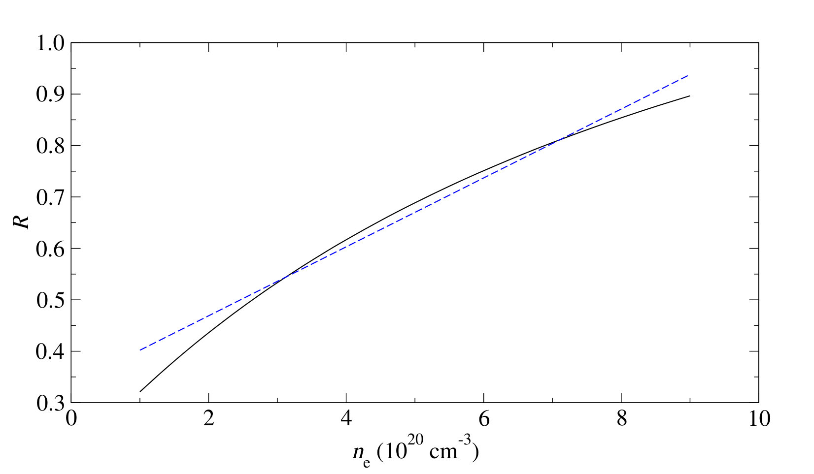 Figure 1
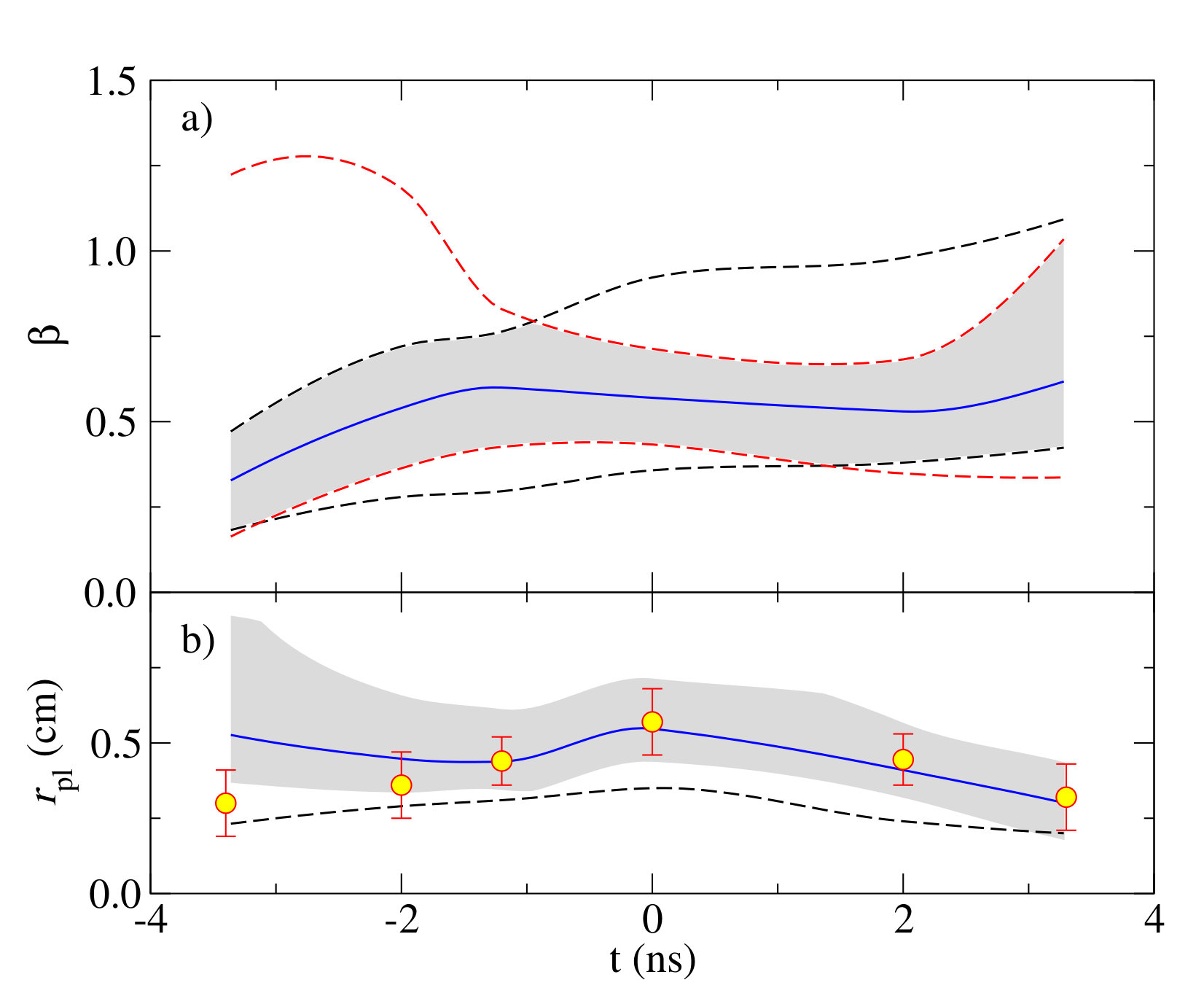 Figure 2
| Experimental data | Uniform plasma | Isothermal turbulence | ||||||||||||||||
| t (ns) | (GW) | Re | ||||||||||||||||
| -3.4 | 0.15 | 0.19 | 0.41 | 3000 | 0.23 | 6.0 | 120 | 250 | 2.4 | 0.048 | 0.70 | 1.84 | 5.77 | 0.32 | 1.9 | 0.53 | ||
| -2.0 | 0.15 | 0.25 | 0.47 | 2100 | 0.29 | 6.0 | 175 | 230 | 1.7 | 0.034 | 0.40 | 1.44 | 2.86 | 0.54 | 3.2 | 0.45 | ||
| -1.2 | 0.15 | 0.36 | 0.52 | 1800 | 0.31 | 6.0 | 190 | 210 | 1.6 | 0.032 | 0.36 | 1.39 | 2.60 | 0.60 | 3.6 | 0.44 | ||
| 0.0 | 0.15 | 0.46 | 0.68 | 1300 | 0.35 | 6.0 | 185 | 200 | 1.3 | 0.026 | 0.25 | 1.26 | 1.96 | 0.57 | 3.4 | 0.55 | ||
| 2.0 | 0.15 | 0.36 | 0.53 | 900 | 0.24 | 6.0 | 155 | 180 | 1.2 | 0.024 | 0.21 | 1.22 | 1.80 | 0.53 | 3.2 | 0.41 | ||
| 3.3 | 0.15 | 0.21 | 0.43 | 720 | 0.20 | 6.0 | 140 | 180 | 1.0 | 0.020 | 0.15 | 1.16 | 1.53 | 0.62 | 3.7 | 0.30 | ||
Peer Reviews
No public reviews on file for this paper yet. If you reviewed it on a platform where reviews are public (OpenReview, ICLR, NeurIPS, ICML), you can paste yours below so the community can read it here.
Videos
No videos yet. Explain this paper in a talk, walkthrough, or lecture? Add one.
Present address: ] Tri Alpha Energy Inc, Foothill Ranch, CA, USA
Present address: ] Applied Materials, Rehovot, Israel
Turbulent stagnation in a z-pinch plasma
E. Kroupp
E. Stambulchik
Corresponding author: [email protected]
A. Starobinets
D. Osin
[
V. I. Fisher
D. Alumot
[
Y. Maron
Faculty of Physics, Weizmann Institute of Science, Rehovot 7610001, Israel
S. Davidovits
Corresponding author: [email protected]
N. J. Fisch
Princeton University, Princeton, New Jersey 08540, USA
A. Fruchtman
H.I.T.—Holon Institute of Technology, Holon 5810201, Israel
Abstract
The ion kinetic energy in a stagnating plasma was previously determined by Kroupp et al., \BibitemOpen\bibfieldjournal Phys. Rev. Lett. 107, 105001 (2011)\BibitemShutNoStop, from Doppler-dominated lineshapes augmented by measurements of plasma properties and assuming a uniform-plasma model. Notably, the energy was found to be dominantly stored in hydrodynamic flow. Here, we advance a new description of this stagnation as supersonically turbulent. Such turbulence implies a non-uniform density distribution. We demonstrate how to re-analyze the spectroscopic data consistent with the turbulent picture, and show this leads to better concordance of the overconstrained spectroscopic measurements, while also substantially lowering the inferred mean density.
pacs:
52.58.Lq,52.70.La,52.35.Ra,32.70.-n
Introduction — In implosions of a cylindrical z-pinch plasma, hydrodynamic kinetic motion is ultimately transferred to thermal motion of plasma particles—electrons and ions—through a cascade of atomic and thermodynamic processes Ryutov et al. (2000); Slutz and Vesey (2012); Herrmann (2014); Sinars et al. (2016). These processes culminate at the stagnation phase, producing high-energy-density plasmas and generating powerful x-ray and neutron radiation Giuliani and Safronova (2016).
Previous x-ray spectroscopic analysis of pinch plasmas Kroupp et al. (2011); Maron et al. (2013) found that the ion kinetic energy at the stagnation phase was dominantly non-thermal hydrodynamic motion, while the plasma appeared largely uniform at spatial and temporal scales down to at least and 1 ns, respectively. An explanation of this phenomenon has been offered Giuliani et al. (2014), where simulations showed steep radial velocity gradients in the stagnation region. On the other hand, we note here that the Reynolds number in the stagnating plasma is initially high (), making turbulence a candidate for such significant small-scale hydrodynamic motion (the 2D simulations in Giuliani et al. (2014) would not be expected to reproduce turbulent behavior). The inferred Mach numbers, , at stagnation are supersonic, see Table 1 for Re and . Were supersonic turbulence present, it would imply substantial nonuniformity in quantities such as the density (see, e.g., Fig. 2 in (Federrath, C. et al., 2010)). However, the previous analysis Kroupp et al. (2011) assumed a uniform plasma.
This study re-analyzes the experimental data Kroupp et al. (2011) without assuming uniformity, using, instead, a modeled turbulent density distribution Hopkins (2013). In doing so, we give both a new physical description of a stagnated plasma dominated by supersonic turbulence, and a new spectroscopic analysis method. We find full (actually, improved) consistency with the observations, but a significantly (about two-fold) lower average density. The results are believed to also be relevant for large-scale z-pinch devices, inertial confinement experiments with large residual hydrodynamic motion, and in various astrophysical contexts.
Short description of the previous study — In brief, a 9-mm-long neon-puff z-pinch was imploded in 500 ns under a current rising to 500 kA at the stagnation time. Experimental diagnostics included high-resolution (\sim$$200\,\mathrm{\upmu\mathrm{m}}) gated x-ray filtered-pinhole imaging, a spectrometer recording Ne He-like dielectronic satellites with a resolving power of 6700, and a photo-conductive detector (PCD) sensitive to radiation. All the data were simultaneously acquired over the stagnation period, about around the peak of the PCD signal with a time resolution of 1 ns. A plasma segment at along the pinch axis was used for the analysis.
The modeling assumed a uniform-cylinder plasma with a prescribed (within experimental uncertainties) time evolution of , , and plasma radius . The experimental data and uniform model parameters are shown in Table 1. Assuming uniformity, the electron density was determined based on the satellite-intensity ratio Seely (1979); Kroupp et al. (2007); it is in the table. A separately measured time-integrated continuum slope Alumot (2007) was found to agree with the assumed. The x-ray images give to within the \sim$$200\,\mathrm{\upmu\mathrm{m}} resolution, in Table 1. The self-consistency of the uniform-model time dependencies for , and was verified using the additional measurement of the absolutely calibrated PCD signal, which is sensitive to all three quantities. With fixed, it was found that either or could be taken at the center of its measured value range (i.e. uncertainty), with the other quantity then within one or two standard deviations of its independently measured value. With the more important quantity, it was chosen to let vary outside one deviation; this gave in Table 1.
New model — Although the uniform plasma analysis was reasonably consistent with the data, the uniform density assumption will not be physically sound if the plasma is highly turbulent, as expected for the measured Re and . Therefore, we use a (non-uniform) turbulent plasma model. Within such a model, all plasma properties—density , electron and ion temperatures, and the non-thermal ion velocity —have certain distributions, with possible correlations between them. This work analyzes the simplest case, of isothermal turbulence, where and are uniform (see the discussion below), whereas (and ) are not. Then, the previous spectral fits and analysis are still valid because: the correlation between turbulent velocity and density is very weak for isothermal turbulence Federrath, C. et al. (2010); and the turbulent velocity distribution is well approximated by a Gaussian (see, e.g. Smith et al. (2000); Porter et al. (2002); Kitsionas et al. (2009)), which was also the assumed non-thermal velocity distribution used in the original study Kroupp et al. (2011). This leaves inferred from Doppler broadening Kroupp et al. (2007) unaffected. We now show that, using a turbulent density probability distribution function (PDF) that is consistent with the measured and , the inferred density is substantially reduced, which allows the inferred plasma radius at each time to be larger, while staying consistent with the PCD signal. This larger radius now agrees well with (except at the first measurement time, which has the weakest signal). Thus, the new turbulent model is an improvement both because it is physically sound and gives an improved match to the observations.
We work with electron density instead of mass density , since the atomic experimental data are sensitive to . The two are related, , where is the mean ion charge and is the ion mass. In principle, is a function of and , but for the ranges of plasma parameters of interest, it varies very weakly Kroupp et al. (2011); Giuliani et al. (2014), so we assume .
For each measurement the density has a PDF, . The previous data analysis Kroupp et al. (2011) corresponds to . ’s are different at different times and -positions, i.e., ; for brevity, these labels will be omitted.
Let us switch to dimensionless quantity
[TABLE]
The average density is . It is important to note that is not the same as . The nonuniform density affects two of the previous measurements: from line ratios and the absolutely calibrated PCD signal, from which one can infer the radiating mass (product of and ), for a given . These measurements give two constraints on the turbulent PDF, , which thus determine the new mean density.
Assuming the collisional-radiative equilibrium is established much faster than the hydromotion, the intensity of a discrete spectral line or continuum radiation in a turbulent plasma can be obtained in the static approximation Stamm et al. (2017), viz.,
[TABLE]
Here, is the local plasma emissivity, approximately scaling as if the density does not vary too much, is the length (in the direction) of the plasma segment being analyzed, and we assumed that density variations are independent of . In particular, the PCD signal is
[TABLE]
Using this, and the fact that the previous model described self-consistently (within the errors bars ) by assuming , we can get a first constraint on , bounding with and and ,
[TABLE]
Some of the autoionizing dielectronic satellites have even stronger density dependence than —which is why the intensity ratio of such a satellite to another line (in our case—another close-by dielectronic satellite) allows for inferring the density Seely (1979). Both dependencies are complex, but around the density point of interest (), their ratio is rather close to a linear form, , in a steady-state optically thin plasma (see Fig. 1). Hence, if does not vary too wildly, (say, within a factor in each direction),
[TABLE]
The measured quantity is known within its error bars, i.e., . Therefore, Eq. (5) gives a second constraint on ,
[TABLE]
To model the density PDF that would result from turbulence in the stagnating plasma, we use the PDF of Hopkins (2013). Since the model assumes the average density is known, it is convenient to introduce dimensionless volumetric density by normalizing to , i.e., . Evidently, . In terms of , the (volumetric) PDF is
[TABLE]
where , and , and is the modified Bessel function of the first kind. This two-parameter PDF depends on a variance, , and a measure of intermittency, . As , the PDF becomes lognormal. This PDF fits well for simulations conducted at a wide range of Mach numbers Hopkins (2013). Although we presently treat the turbulence as isothermal, this PDF has been shown to fit for simulations of non-isothermal turbulence Federrath and Banerjee (2015). In general, the values of, , , depend on the turbulence properties; they are typically modeled as depending on the turbulent Mach number, the mix of compressive and solenoidal forcing, and, in the non-isothermal case, the polytropic gamma Hopkins (2013); Federrath and Banerjee (2015). As such, the turbulence model does not introduce any “free” parameters, since its parameters vary only as a direct consequence of the variation of measured or inferred plasma properties.
For the value of , we use the fit to simulation data Hopkins (2013), which is . Here is the compressive Mach number, also written Konstandin et al. (2012, 2016), and is related to the mix of solenoidal and compressive modes Federrath et al. (2008); Konstandin et al. (2012, 2016). For the density variance, , we combine the usual isothermal logarithmic density variance (see, e.g., (Padoan et al., 1997; Passot and Vázquez-Semadeni, 1998; Padoan and Nordlund, 2011; Molina et al., 2012)), , with the relationships (Hopkins, 2013) and (Federrath and Banerjee, 2015). This yields . Here we take ; see the discussion below for more on this choice, and caveats associated with the turbulence model.
The Mach number at each time is calculated using the data in Table 1; , where and , where is used, assuming isothermality (discussed below).
Results and discussion — We now use the turbulent density PDF, Eq. (7), in the constraints (4) and (6). In addition to satisfying the usual normalization condition, Eq. (1), it also conserves the average density, . However, experimentally the average density is unknown; in order to use the volumetric PDF and its moments, we connect and with a free parameter , . Once the turbulence PDF satisfying the experimental data within the constraints (4) and (6) is determined, will give the new mean density, corrected for the presence of turbulence; more generally, . With this in mind, Eqs. (4) and (6) become a set of inequalities on ,
[TABLE]
shown graphically in Fig. 2a. The new model predicts a significantly (about two-fold) lower average density. With chosen, the plasma radius needs to be corrected, accounting for the turbulence-modified average emissivity. Using Eq. (3), it follows that . Notably, ’s in the present model (listed as in Table 1) fit the measured values better than the original model Kroupp et al. (2011), as shown in Fig. 2b.
For clarity, we have presented results in Fig. 2 with only experimental uncertainty. There are also uncertainties associated with the turbulence model. Changes in the results due to most of these uncertainties are primarily expected to be quantitative, with the picture of reduced mean density remaining. One uncertainty comes from the possibly non-equilibrium nature of any turbulence at stagnation. The turbulent velocity decreases in time during stagnation, as evidenced by the decreasing non-thermal energy excess per-ion () in Table 1. However, contrary to the turbulence simulations usually considered for modeling (e.g. in (Hopkins, 2013)), the total mass is not constant in time: at least initially, plasma continues to flow into the stagnation region. Using the isothermal turbulence and in Table 1, , , along with a turbulent energy per particle of , yields a total turbulent energy in the stagnation region that remains relatively constant from ns to ns, then falls. Notably, the timescale for this observed fall (a few ns) is the dynamical timescale expected for supersonic turbulence (Mac Low et al., 1998; Mac Low, 1999) with these flow speeds and length scales; importantly, it is much faster than the viscous timescale, without a cascade. Although the present density PDF model works in a variety of cases, it has typically been tested in situations with equilibrium forcing, which may not be the best analog for the present case.
Assuming the model applies, there are still uncertainties. One is the degree to which turbulence in this stagnating plasma would be isothermal. Conduction and turbulent timescales are not well-separated, so that an accurate determination of the degree of isothermality would likely require detailed simulations, as in other topic areas (Pavlovski et al., 2002, 2006). The turbulence model used here applies in the non-isothermal case, with different , (Federrath and Banerjee, 2015). At this level, non-isothermality is expected to only modestly change the parameters in Table 1, although then the inferred and will also need to be reconsidered, because non-isothermality would have a pronounced effect on the local plasma emissivity (it depends rather strongly on ), requiring modifications to Eqs. (2) and (5)—and therefore also to (8) and (9).
Any magnetic fields in the stagnating region could alter the values of and (Padoan and Nordlund, 2011; Molina et al., 2012; Hopkins, 2013), although the form of the PDF remains valid. These corrections should be small because the plasma pressure is much higher than the magnetic pressure in the stagnation region () Rosenzweig et al. (2014).
Even within the isothermal turbulence PDF model, there are uncertainties. Simulations show substantial spread in values of the PDF parameters around the expressions for and , see, e.g., Hopkins (2013). Apart from modeling errors, spread in these values can be physical, due to the fluctuations of turbulence (Lemaster and Stone, 2008). The correct value of , presently taken to be , is uncertain. Generally, (Federrath et al., 2008; Federrath, C. et al., 2010), with occurring for solenoidal (divergence free) forcing (Federrath et al., 2008) and occuring for compressive (curl-free) forcing. Equal parts solenoidal and compressive forcing gives (Federrath, C. et al., 2010). For a z-pinch, one might expect largely compressive forcing. Given this uncertainty, one could calculate the range of in Fig. 2a including also uncertainty in . A larger yields a lower range for , while a smaller yields a higher range.
The ion temperatures in Table 1 are inferred through a calculation involving the electron–ion temperature equilibration time (Kroupp et al., 2011). Since this time is density dependent, it will be affected by density fluctuations. The equilibration timescale is faster in the high density regions, which dominate the measurements, thus, the ion temperature may be driven slightly closer to the electron temperature. Since the electron–ion temperature equilibration timescale is already very fast, this is expected to cause to be a few percent lower than in Ref. Kroupp et al. (2011).
The underlying atomic model used for the present analysis is the same as in the previous study Kroupp et al. (2011) and, therefore, no additional uncertainties have been introduced. In fact, the associated inaccuracy may be surprisingly low, as the Monte-Carlo analysis of uncertainty propagation in collisional-radiative models indicates Ralchenko (2016). So far, we have neglected possible opacity effects. Fortunately, the satellites used have a negligible optical thickness. The bound–free and free–free (bremsstrahlung) radiation that contributes to the PCD signal is also optically thin, however strong bound–bound transitions are not. This requires a modification of Eq. (2) which cannot be represented analytically. However, the plasma absorption coefficients, similar to the emission ones, for these transitions scale as . Therefore, the difference from the uniform-plasma model (in which the opacity was properly accounted for numerically) should vanish in the lowest order.
The mechanism generating the (non-radial) hydrodynamic motion is unclear; while energy is dumped in the hydrodynamic motion in the process of stagnation (Maron et al., 2013), this hydrodynamic motion could be seeded by turbulence generated and carried along during the compression itself, or could be generated entirely at stagnation. In either event, there are important implications, both for z-pinches, and more broadly.
If the (turbulent) hydromotion is generated and carried along during the compression, these z-pinches represent a test bed for the properties of plasma turbulence undergoing compression. These properties are relevant for a proposed novel fast ignition or x-ray burst generation scheme (Davidovits and Fisch, 2016a, b). Of particular interest is that the present hydromotion is supersonic, the regime in which these schemes would operate. Further, the behavior of compressing supersonic turbulence is of critical interest in astrophysics, particularly for molecular cloud dynamics (Robertson and Goldreich, 2012; Davidovits and Fisch, 2017). Supersonic turbulence behavior has been related to the star formation efficiency (Elmegreen, 2008), the core mass/stellar initial mass functions (Padoan and Nordlund, 2002; Ballesteros-Paredes et al., 2006; Hennebelle and Chabrier, 2008), and Larson’s laws (Kritsuk et al., 2013).
If the hydrodynamic motion is generated at stagnation, and then decays, its properties could still be of astrophysical interest (see, e.g., (Mac Low et al., 1998; Mac Low, 1999; Smith et al., 2000; Ostriker et al., 2001; Pavlovski et al., 2002, 2006; Lemaster and Stone, 2008; Kitsionas et al., 2009; Davidovits and Fisch, 2017)). To the extent generation and/or decay of the hydrodynamic motion at stagnation can be observed, studies of supersonic turbulence in z-pinches could serve as a new and important area for laboratory astrophysics. Indeed, in the present study, not all values of the turbulent PDF parameters, , will be consistent with the observations; more measurements could help to constrain turbulent properties. Z-pinches such as the present may yield other cross-over opportunities with astrophysics, for example, in turbulent density PDF measurement techniques (e.g. Ostriker et al. (2001); Brunt et al. (2010)), or in mechanisms for turbulent generation and forcing in complex plasma environments (e.g. Gritschneder et al. (2009)).
The present analysis is likely relevant to high-current implosions, like z-pinch experiments on the Z machine Jones et al. (2006). Indeed, based on the plasma parameters given in Maron et al. (2013), Re is also high (), and M is similar to the case analyzed here. This analysis may also be relevant in inertial confinement experiments that observe large quantities of residual hydrodynamic motion.
Even though the present experiments are very well diagnosed by z-pinch standards, one should consider additional measurements for verifying the picture of a turbulent stagnation. To this end, other spectroscopy methods can be useful. For example, one can try to study the density by the use of the Stark broadening of high- transitions in hydrogen-like Ne or lower- species (C, N, or O) that can be mixed with the puffed neon.
In summary, a new analysis of stagnating pinch data, replacing the assumption of uniform plasma with density variations consistent with a turbulent plasma, advances a picture of supersonically turbulent stagnating plasma. This picture is not only consistent with the observations, it improves the agreement with them. The mean plasma density is reduced by a factor 2. While there is uncertainty in the precise value of this reduction, the general picture, of a data analysis in the presence of highly turbulent stagnating plasma reducing the inferred stagnation density compared to the uniform case, is believed to be robust and widely relevant. Beyond aiding our understanding of z-pinches, we hope this study has shown fertile ground for relation to problems of astrophysical interest.
Acknowledgements.
Y.M. is grateful to M. Herrmann, A. L. Velikovich, and E. P. Yu for enlightening discussions. This work was supported by BSF–NSF (USA) and BSF 2014714. The work of E.K., E.S., A.S., V.I.F., and Y.M. was supported in part by the Israel Science Foundation and the DOE–Cornell University Excellence Center (USA). The work of S.D. and N.J.F. was supported by NNSA 67350-9960 (Prime # DOE DE-NA0001836) and by NSF Contract No. PHY-1506122.
The reference list from the paper itself. Each links out to its DOI / PubMed record.
- 1Ryutov et al. (2000) \Bibitem Open \bibfield author D. D. Ryutov, M. S. Derzon, and M. K. Matzen, \bibfield journal Rev. Mod. Phys. 72 , 167 (2000) \Bibitem Shut No Stop
- 2Slutz and Vesey (2012) \Bibitem Open \bibfield author S. A. Slutz and R. A. Vesey, \bibfield journal Phys. Rev. Lett. 108 , 025003 (2012) \Bibitem Shut No Stop
- 3Herrmann (2014) \Bibitem Open \bibfield author M. Herrmann, \bibfield journal Nature 506 , 302 (2014) \Bibitem Shut No Stop
- 4Sinars et al. (2016) \Bibitem Open \bibfield author D. B. Sinars, E. M. Campbell, M. E. Cuneo, C. A. Jennings, K. J. Peterson, and A. B. Sefkow, \bibfield journal J. Fusion Energ. 35 , 78 (2016) \Bibitem Shut No Stop
- 5Giuliani and Safronova (2016) \Bibitem Open \bibfield author J. L. Giuliani and A. S. Safronova, \bibfield journal Phys. Plasmas 23 , 101101 (2016) \Bibitem Shut No Stop
- 6Kroupp et al. (2011) \Bibitem Open \bibfield author E. Kroupp, D. Osin, A. Starobinets, V. Fisher, V. Bernshtam, L. Weingarten, Y. Maron, I. Uschmann, E. Förster, A. Fisher, M. E. Cuneo, C. Deeney, and J. L. Giuliani, \bibfield journal Phys. Rev. Lett. 107 , 105001 (2011) \Bibitem Shut No Stop
- 7Maron et al. (2013) \Bibitem Open \bibfield author Y. Maron, A. Starobinets, V. I. Fisher, E. Kroupp, D. Osin, A. Fisher, C. Deeney, C. A. Coverdale, P. D. Lepell, E. P. Yu, C. Jennings, M. E. Cuneo, M. C. Herrmann, J. L. Porter, T. A. Mehlhorn, and J. P. Apruzese, \bibfield journal Phys. Rev. Lett. 111 , 035001 (2013) \Bibitem Shut No Stop
- 8Giuliani et al. (2014) \Bibitem Open \bibfield author J. L. Giuliani, J. W. Thornhill, E. Kroupp, D. Osin, Y. Maron, A. Dasgupta, J. P. Apruzese, A. L. Velikovich, Y. K. Chong, A. Starobinets, V. Fisher, Yu. Zarnitsky, V. Bernshtam, A. Fisher, T. A. Mehlhorn, and C. Deeney, \bibfield journal Phys. Plasmas 21 , 031209 (2014) \Bibitem Shut No Stop