Distributed Control for Spatial Self-Organization of Multi-Agent Swarms
Vishaal Krishnan, Sonia Mart\'inez

TL;DR
This paper presents a distributed control approach for multi-agent swarms to self-organize spatially without position data, achieving desired density distributions in 1D and 2D domains using Laplacian-based algorithms.
Contribution
It introduces a novel pseudo-localization method and control laws enabling swarms to self-organize spatially without position information, applicable in both 1D and 2D.
Findings
Successful design of distributed control laws for density shaping.
Effective pseudo-localization algorithm for agents without position data.
Validation of methods in both 1D and 2D spatial domains.
Abstract
In this work, we design distributed control laws for spatial self-organization of multi-agent swarms in 1D and 2D spatial domains. The objective is to achieve a desired density distribution over a simply-connected spatial domain. Since individual agents in a swarm are not themselves of interest and we are concerned only with the macroscopic objective, we view the network of agents in the swarm as a discrete approximation of a continuous medium and design control laws to shape the density distribution of the continuous medium. The key feature of this work is that the agents in the swarm do not have access to position information. Each individual agent is capable of measuring the current local density of agents and can communicate with its spatial neighbors. The network of agents implement a Laplacian-based distributed algorithm, which we call pseudo-localization, to localize themselves…
Click any figure to enlarge with its caption.
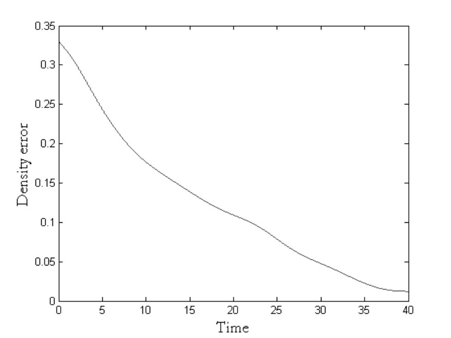 Figure 1
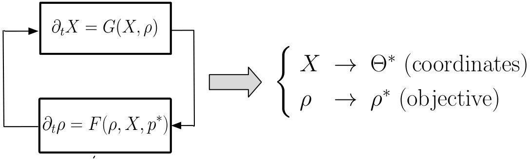 Figure 2
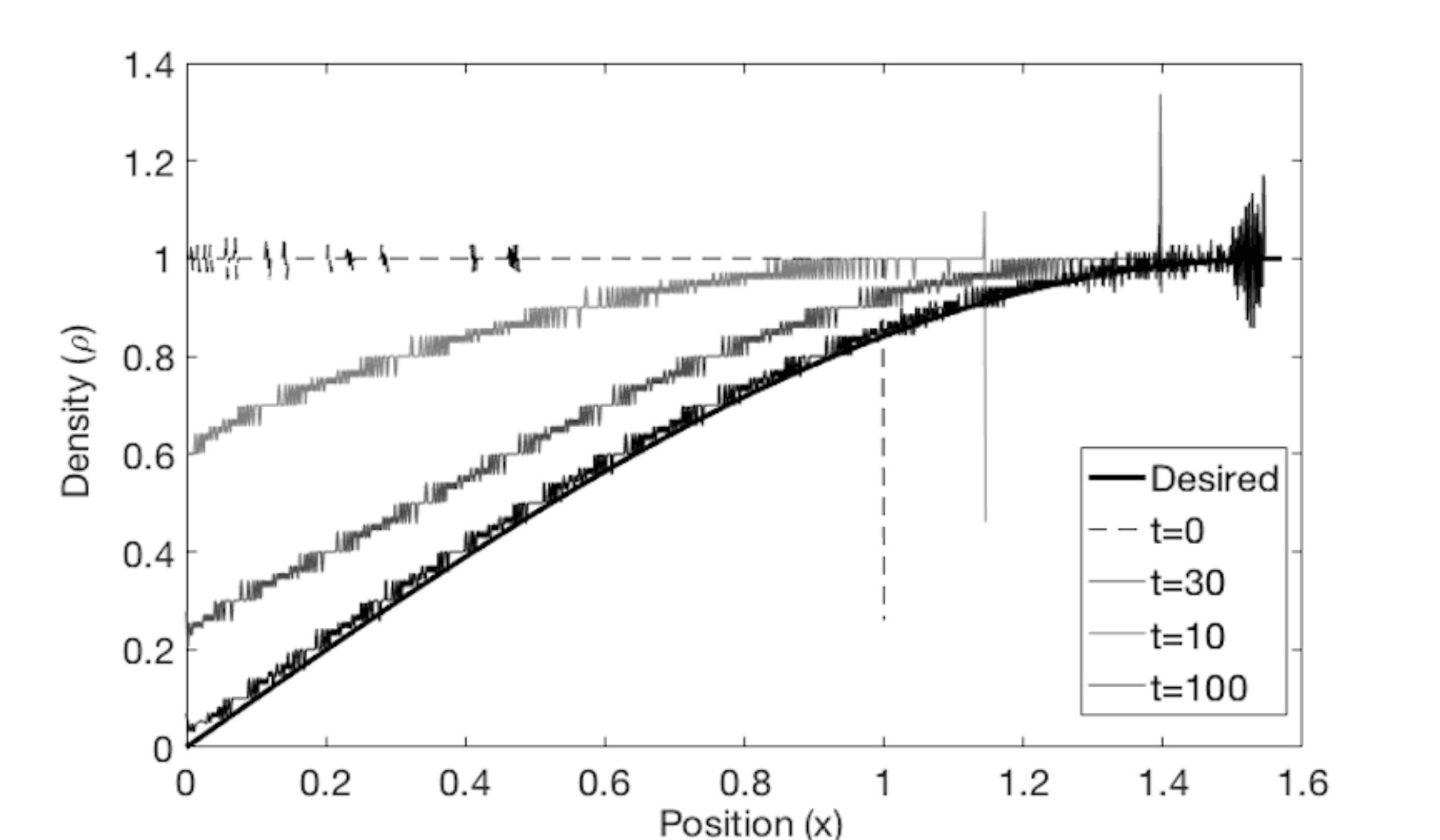 Figure 3
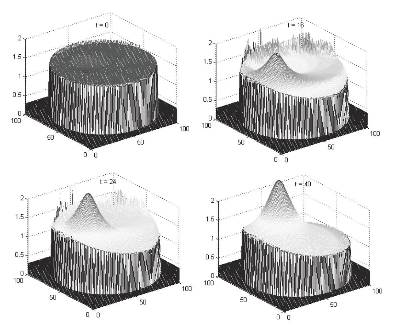 Figure 4
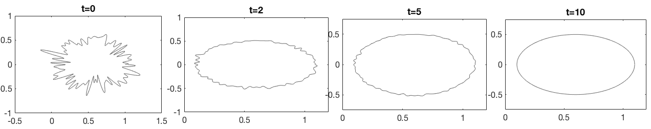 Figure 5
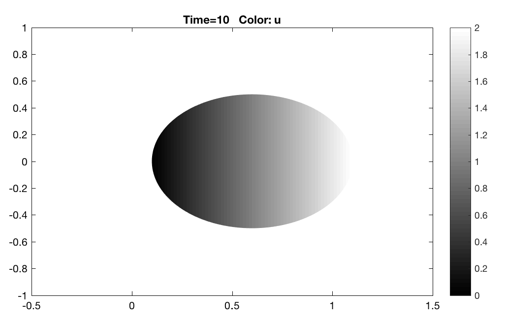 Figure 6
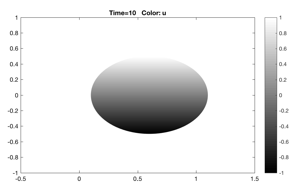 Figure 7
Peer Reviews
No public reviews on file for this paper yet. If you reviewed it on a platform where reviews are public (OpenReview, ICLR, NeurIPS, ICML), you can paste yours below so the community can read it here.
Videos
No videos yet. Explain this paper in a talk, walkthrough, or lecture? Add one.
\newsiamthm
claimClaim \newsiamremarkremRemark \newsiamremarkexplExample \newsiamremarkhypothesisHypothesis
\newsiamremarkassumptionAssumption
Distributed Control for Spatial Self-Organization of Multi-Agent Swarms††thanks: This work has been partially supported by grant FA9550-18-1-0158.
Vishaal Krishnan and Sonia Martínez The authors are with the Department of Mechanical and Aerospace Engineering, University of California at San Diego, La Jolla CA 92093 USA (email: [email protected]; [email protected]).
Abstract
In this work, we design distributed control laws for spatial self-organization of multi-agent swarms in 1D and 2D spatial domains. The objective is to achieve a desired density distribution over a simply-connected spatial domain. Since individual agents in a swarm are not themselves of interest and we are concerned only with the macroscopic objective, we view the network of agents in the swarm as a discrete approximation of a continuous medium and design control laws to shape the density distribution of the continuous medium. The key feature of this work is that the agents in the swarm do not have access to position information. Each individual agent is capable of measuring the current local density of agents and can communicate with its spatial neighbors. The network of agents implement a Laplacian-based distributed algorithm, which we call pseudo-localization, to localize themselves in a new coordinate frame, and a distributed control law to converge to the desired spatial density distribution. We start by studying self-organization in one-dimension, which is then followed by the two-dimensional case.
keywords:
Self-organization, Distributed control, Pseudo-localization, Harmonic maps
{AMS}
34B45, 35B40, 35B35, 58J32, 58J35, 58E20
1 Introduction
Self-organization in swarms refers broadly to the emergence of patterns of long-range order in large groups of dynamic agents which interact locally with each other. It is a pervasive phenomenon in nature, observed in biological [7] and other natural systems [36]. In the context of robotic systems, problems of deployment and formation control of groups of robots have been extensively studied [6, 27, 11, 32, 21]. More recently, research efforts have been undertaken to massively increase the scale of these robotic systems [30]. This transition does not merely involve an increase in the size of robotic networks, but it also introduces new theoretical challenges for their analysis and control design. In particular, large groups of agents have some essential characteristics that distinguish them from other smaller-scale counterparts. In a swarm, individual agents have no significance and only the macroscopic objectives are relevant. A swarm largely remains unaffected by the removal of a large, but discrete, number of agents. Moreover, it is difficult (and needlessly complicated) to specify the global configuration of the swarm using the states of individual agents; instead, employing macroscopic quantities such as the swarm spatial density distribution to specify its configuration is more appropriate. From an analysis and control-theoretic viewpoint, the dynamic modeling of swarms is less explored, which e.g. can be established by means of PDEs, for which control theoretic tools are less well developed in comparison to ODEs. These theoretical challenges motivate the investigation of self-organization in large-scale swarms.
In the literature, Markov-chain based methods have been widely used in addressing some of the key theoretical problems pertaining to swarm self-organization. By means of it, the swarm configuration is described through the partitioning the spatial domain in a finite number of larger size disjoint subregions, on which a probability distribution is defined. Then, the self-organization problem is reduced to the design of the transition matrix governing the evolution of this probability density function to ensure its convergence to a desired profile. A recent approach to density control using Markov chains is presented in [12], which includes additional conflict-avoidance constraints. In this setting every agent is able to determine the bin to which it belongs at every instant of time, which essentially means that individual agents have self-localization capabilities. Also, the dimensional transition matrix is synthesized in a central way at every instant of time by solving a convex optimization problem. In [3], the authors make use of inhomogeneous Markov chains to minimize the number of transitions to achieve a swarm formation. In this approach, the algorithm necessitates the estimation of the current swarm distribution, and computes the transition Markov matrices for each agent, at each instant of time. The fact that every agent needs to have an estimate of the global state (swarm distribution) at every time may not be desirable or feasible. The localization of each agent still remains to be a main assumption. Under similar conditions, one can find the manuscripts [1] and [8], which describe probabilistic swarm guidance algorithms. In [5], the authors present an approach to task allocation for a homogeneous swarm of robots. This is a Markov-chain based approach, where the goal is to converge to the desired population distribution over the set of tasks.
In the context of robotic swarms, programmable self-assembly of two-dimensional shapes with a thousand-robot swarm is demonstrated in [31]. These robots are capable of measuring distances to nearby neighbors which they use to localize themselves relative to other localized robots. Each robot then uses its position to implement an edge-following algorithm.
Another approach uses partial differential equations to model swarm behaviour, and control action is applied along the boundary of the swarm. Previous works on PDE-based methods with boundary control include [18], where the authors present an algorithm for the deployment of agents onto families of planar curves. Here, the swarm collective dynamics are modeled by the reaction-advection-diffusion PDE and the particular family of curves to which the swarm is controlled to is parametrized by the continuous agent identity in the interval of unit length. An extension of this work to deployment on a family of D surfaces in D space can be found in [29]. The problem of planning and task allocation is addressed in the framework of advection-diffusion-reaction PDEs in [14]. In [17] and [16], the authors present an optimal control problem formulation for swarm systems, where microscopic control laws are derived from the optimal macroscopic description using a potential function approach.
The problem of position-free extremum-seeking of an external scalar signal using a swarm of autonomous vehicles, inspired by bacterial chemotaxis, has been studied in [28].
In this work, we adopt a viewpoint outlined in [2], wherein we make an amorphous medium abstraction of the swarm, which is essentially a manifold with an agent located at each point. We then model the system using PDEs and design distributed control laws for them. An important component of this paper is the Laplacian-based distributed algorithm which we call pseudo-localization algorithm, which the agents implement to localize themselves in a new coordinate frame. The convergence properties of the graph Laplacian to the manifold Laplacian have been studied in [4], which find useful applications in this paper.
The main contribution of this paper is the development of distributed control laws for the index- and position-free density control of swarms to achieve general 1D and a large class of 2D density profiles. In very large swarms with thousands of agents, particularly those deployed indoors or at smaller scales, presupposing the availability of position information or pre-assignment of indices to individual agents would be a strong assumption. In this paper, in addition to not making the above assumptions, the agents are only capable of measuring the local density, and in the D case, the density gradient and the normal direction to the boundary.
Under these assumptions, we present distributed pseudo-localization algorithms for one and two dimensions that agents implement to compute their position identifiers. Since every agent occupies a unique spatial position, we are able to rigorously characterize the resulting position assignment as a one-to-one correspondence between the set of spatial coordinates and the set of position identifiers, which corresponds to a diffeomorphism of the continuum domain. Based on this assignment, we then design control strategies for self-organization in one and two dimensions under the assumption that the motion control of agents is noiseless. The extension to the D case leads to new difficulties related to the control of the swarm boundaries. To address these, we implement a variant of the D pseudo-localization algorithm at the boundary during an initialization phase. A preliminary version of this work appeared in [23] where we presented an outline of the algorithms and stated some of the results. We develop them here rigorously, providing detailed proofs for our claims.
The paper is organized as follows. In Section 2, we introduce the basic notation and preliminary concepts used in the manuscript. We present the analysis of self-organization in one dimension in Section 4, where we introduce the pseudo-localization algorithm in Section 4.1 and the distributed control law in Section 4.2. After this, we generalize and extend the analysis for self-organization in two dimensions in Section 5. Section 6 contains numerical simulations of the results in the paper, and in Section 7, we present our conclusions.
2 Preliminaries
Let denote the set of all real numbers, the set of non-negative real numbers, and n the -dimensional Euclidean space. We use boldface letters to denote vectors in n. The norm of a vector is the standard Euclidean -norm, unless otherwise specified. Let denote the gradient operator in n when acting on real-valued functions and the Jacobian in the context of vector-valued functions. As a shorthand, we let for a variable . Let be the Laplace operator in n. We denote by either or the total time derivative of . Given functions , we write if there exist positive constants and such that , for all . Let denote the set of agents in the swarm, and its cardinality. For the D case, let denote the leftmost agent, and the rightmost one. Let denote the spatial neighborhood of agent , which comprises those agents located inside a small ball centered at . A set-valued mapping, denoted by , maps the set of real numbers onto subsets of 2. For a bounded open set , denotes its boundary, its closure and its interior with respect to the standard Euclidean topology. The set of smooth real-valued functions on is denoted by . We let (or in 1D) denote the standard Lebesgue measure; with a slight abuse of notation, we sometimes omit (resp. in 1D) from long integrals. The Dirac measure on defined for any and any measurable set is given by for , and for .
For two non-empty subsets and of a metric space , the Hausdorff distance between them is defined as:
[TABLE]
On a measurable space , let constitute the space, where is the norm. Of particular interest is the space, or the space of square-integrable functions. In this paper, we denote by the norm of with respect to the Lebesgue measure, and by the weighted norm (with the strictly positive weight on ). The Sobolev space over a measurable space is defined as . Of particular interest is the space , also called the space. For two functions and , we denote by the convergence in norm (over the domain of the functions) of to as , that is, . Convergence in norm is denoted similarly by .
We now state some well-known results that we will be used in the subsequent sections of this paper.
Lemma 2.1**.**
(Divergence Theorem [10]). For a smooth vector field over a bounded open set with boundary , the volume integral of the divergence of over is equal to the surface integral of over :
[TABLE]
where is the outward normal to the boundary and the measure on the boundary. For a scalar field and a vector field defined over :
[TABLE]
Lemma 2.2**.**
*(Leibniz Integral Rule [10]).
Let and be a smooth one-parameter family of bounded open sets in n generated by the flow corresponding to the smooth vector field on n. Then:*
[TABLE]
Corollary 2.3**.**
*(Derivative of Energy Functional).
Let be an energy functional defined as follows:*
[TABLE]
for some function . Then,
[TABLE]
where is the total derivative.
Proof 2.4**.**
We have included the proof for this corollary for the sake of completeness. Using the Leibniz integral rule and the Divergence theorem, we have (it is understood that the integrations are with respect to the measure ):
[TABLE]
Lemma 2.5**.**
*(Poincaré-Wirtinger Inequality [26]).
For and , a bounded connected open subset of n with a Lipschitz boundary, there exists a constant depending only on and such that for every function in the Sobolev space :*
[TABLE]
*where , and is the Lebesgue measure of . *
Lemma 2.6**.**
*(Rellich-Kondrachov Compactness Theorem [15]).
Let be open, bounded and such that is . Suppose , then is compactly embedded in for each . In particular, we have is compactly contained in . *
Lemma 2.7**.**
*(LaSalle Invariance Principle [20, 34, 35]).
Let be a continuous semigroup of operators on a Banach space (closed subset of a Banach space with norm ), and for any , define the positive orbit starting from at as . Let be a continuous Lyapunov functional on for (such that in ). Define , and let be the largest invariant subset of . If for , the orbit is pre-compact (lies in a compact subset of ), then , where (where is the distance in ). *
2.1 Continuum model of the swarm
Given that , the number of agents in the swarm, is very large, we will analyze the swarm dynamics through a continuum approximation. Let , and let be a smooth one-parameter family of bounded open sets, such that the agents are deployed over at time . We denote by , , where is the position of the th agent in the swarm at time . Let be the spatial density function supported on for all (with for ), such that . We assume that is simply connected and that the boundary does not self-intersect for all .
Assuming that is smooth, the macroscopic dynamics can now be described by the continuity equation [10], assuming that the total number of agents is conserved:
[TABLE]
where is the velocity field with , such that the one-parameter family is generated by the flow associated with .
2.2 Harmonic maps and diffeomorphisms
Let and be two Riemannian manifolds of dimensions and , and Riemannian metrics and , respectively. A map is called harmonic if it minimizes the functional:
[TABLE]
where is the Riemannian volume form on . The Euler-Lagrange equation for the functional , which also yields the minimum energy, is given by , the Laplace equation [22]. It is useful to note that the solutions to the heat equation, in the limit , approach the harmonic map. This is proved later in Lemma 5.1, and forms the basis for the design of the distributed pseudo-localization algorithm. We now state a lemma on harmonic diffeomorphisms of Riemann surfaces (i.e., above).
Lemma 2.8**.**
*(Harmonic diffeomorphism [13]).
Let be a compact surface with boundary and a compact surface with non-positive curvature. Suppose that is a diffeomorphism onto . Assume that is convex. Then there is a unique harmonic map with on , such that is a diffeomorphism. *
We note that the non-positive curvature constraint in the lemma is essentially a constraint on the metric on , and the curvature is zero for the Euclidean metric.
3 Problem description and conceptual approach
In this section, we provide a high-level description of the proposed problem and explain the conceptual idea behind our approach. The technical details can be found in the following sections.
The problem at hand is to ultimately design a distributed control law for a swarm to converge to a desired configuration. Here, a swarm configuration is a density function of the multi-agent system and the objective is that agents reconfigure themselves into a desired known density . To do this, an agent at position is able to measure the current local density value, ; however, its position within the swarm is unknown. Thus, given , an agent at cannot directly compute nor a feedback law based on . To solve this problem, we devise a mechanism that allows agents to determine their coordinates in a distributed way in an equivalent coordinate system.
Note that, given a diffeomorphism from the spatial domain of the swarm onto the unit interval or disk (i.e. a coordinate transformation), we can equivalently provide the agents with a transformed density function , such that . In this way, instead of the agents are given , but still do not have access to . The pseudo-localization algorithm is a mechanism that agents employ to progressively compute an appropriate (configuration-dependent) diffeomorphism by local interactions.
In 1D, the pseudo-localization algorithm is a continuous-time PDE system in a new variable or pseudo-coordinate which plays the role of an “approximate coordinate” that agents can use to know where they are. The input to this system is the current density value , see Figure 1 for an illustration, and the objective is that converges to a -dependent diffeomorphism. On the other hand, the variable and the function are used to define the control input of another PDE system in the density . In this way, we have a feedback interconnection of two systems, one in and one in , with the goal to achieve (the pseudo-coordinate converges to a true coordinate given by ) and .
As for the control design methodology, we follow a constructive, Lyapunov-based approach to designing distributed control laws for the swarm dynamics modeled by PDEs. For this, we define appropriate non-negative energy functionals that encode the objective and choose control laws that keep the time derivative of the energy functional non-positive. This, along with well-known results on the precompactness of solutions as in Lemma 2.6, the Rellich Kondrachov compactness theorem, allows us to apply the LaSalle Invariance Principle in Lemma 2.7 and other technical arguments to establish the convergence results that we seek.
In the 1D case, we can identify a set of diffeomorphisms associated with any that eventually converge to , and simultaneously control boundary agents into a desired final domain (the support of ). These are given by the cumulative distribution function associated with the density function; see Section 4.1. The 2D case is more complex, and analogous results could not be derived in their full generality. Unlike the 1D case, estimating the cumulative distribution is not straightforward in the 2D case. Instead, we set out to find diffeomorphisms as the result of a distributed algorithm. Given that the discretization of heat flow naturally leads to distributed algorithms, we investigate under what conditions this is the case via harmonic map theory. On the control side, there also are additional difficulties, and because of this, we simplify the control strategy into three stages. In the first stage, the boundary agents are re-positioned onto the boundary of the desired domain while containing the others in the interior. Once this is achieved, the second and third stages can be seen again as the interconnection of two systems in pseudo-coordinates (instead of ) and , analogously to Figure 1. However, we apply a two time-scale separation for analysis by which coordinates are computed in a fast-time scale and reconfiguration is done in a slow-time scale, which allows for a sequential analysis of the two stages. We then study the robustness of this approach. We refer the reader to the extended version of this paper [24] for further description of the discrete implementation.
4 Self-organization in one dimension
In this section, we present our proposed pseudo-localization algorithm and the distributed control law for the D self-organization problem.
For each , let be the interval (with boundary ) in which the agents are distributed in 1D, and let be the normalized density function supported on , for all (with , ), describing the swarm on that interval. Without loss of generality, we place the origin at the leftmost agent of the swarm. We also assume that the leftmost and the rightmost agents, and , are aware that they are at the boundary. Let be the desired normalized density distribution.
Since a direct feedback control law can not be implemented by agents because they do not have access to their positions, we introduce an equivalent representation of the density , , depending on a particular diffeomorphism . First, define such that and .
Now, let , and , be such that .
The function , which represents the desired density distribution mapped onto the unit interval , is computed offline and is broadcasted to the agents prior to the beginning of the self-organization process. We use to derive the distributed control law which the agents implement. We assume that is a Lipschitz function in the sequel. {assumption}(Uniform boundedness of density function). We assume that the density function and its derivative are uniformly bounded in its support, that is, for and there exist uniform lower bounds and uniform upper bounds (where and ) (that is, for all and and for all and ).
4.1 Pseudo-localization algorithm in one dimension
We first consider the static case, that is, the design of the pseudo-localization dynamics on of the upper block in Figure 1, when the agents and are stationary. We define as:
[TABLE]
such that . In other words, is the cumulative distribution function (CDF) associated with . (Note that the domains are static and hence the argument has been dropped, which will be reintroduced later.)
Lemma 4.1**.**
*(The CDF diffeomorphism).
Given , a function, the mapping as defined above, is a diffeomorphism and . *
Proof 4.2**.**
*Since , , it follows that is a strictly increasing function of , and is therefore a one-to-one correspondence on . Moreover, is atleast and has a differentiable inverse, which implies it is a diffeomorphism. Finally, since , we have . *
Our goal here is to set up a partial differential equation with appropriate boundary conditions that yield the diffeomorphism as its asymptotically stable steady-state solution. We begin by setting up the pseudo-localization dynamics for a stationary swarm (for which the spatial domain and the density distribution are fixed). Let be such that , with:
[TABLE]
where is a control input at the boundary and is a control input at the boundary . From (5), we observe that . Letting denote the error, we obtain:
[TABLE]
{assumption}
(Well-posedness of the pseudo-localization dynamics).
We assume that the pseudo-localization dynamics (6) (and (7)) is well-posed, that the solution is sufficiently smooth (at least in the spatial variable, even as ) and belong to the Sobolev space .
Lemma 4.3**.**
*(Pointwise convergence to diffeomorphism). Under Assumption 4.1, on the well-posedness of the pseudo-localization dynamics, and Assumption 4 on the boundedness of , the solutions to PDE (6) converge pointwise to the CDF diffeomorphism defined in (5), as , for all initial conditions . *
In this case, the swarm is stationary, which implies that the distribution is fixed (and so is its support ), and the uniform boundedness assumption 4 simply becomes a boundedness assumption.
Proof 4.4**.**
We prove that the solutions to the PDE (6) converge pointwise to the diffeomorphism by showing that , as , pointwise for (7). For this, we consider a functional , given by (integrations are with respect to the Lebesgue measure):
[TABLE]
The time derivative is given by:
[TABLE]
Here, replace in the first integral with the dynamics in (7), and then use in the second integral together with the Divergence Theorem in Lemma 2.1. We obtain:
[TABLE]
(After the second equal sign, apply again the Divergence Theorem on the first integral of the previous line, and replace from (7).) Substituting from (7), we have:
[TABLE]
*Clearly, , and , for all . Moreover, since and since is uniformly bounded according to Assumption 4, we have that is bounded in . Moreover, by the Rellich-Kondrachov Theorem of Lemma 2.6, is compactly contained in . Then it follows that the solutions are precompact. Thus, by the LaSalle Invariance Principle of Lemma 2.7, the solution to (7) converges in -norm to the largest invariant subset of . Note that implies . Thus, . Since is bounded (), we have , which implies . Now, (since and ). Thus, , for all . Therefore, the solutions to (7) converge to pointwise, as , from any smooth initial . *
We now have that the solution to the pseudo-localization dynamics converges to the diffeomorphism in the stationary case. For the dynamic case, we modify (6) to account for agent motion. Let be supported on for all . Using the relation , where is the velocity field on the spatial domain, we consider:
[TABLE]
In the dynamic case, and w.l.o.g. we have set for all , for simplicity. We will use the above PDE system in the design of the distributed motion control law, redesigning the boundary control to achieve convergence of the entire system. We now discretize (8) to obtain a distributed pseudo-localization algorithm. Let , where is the position of the agent. We identify the agent with its desired coordinate in the unit interval at time , i.e., , where from (5), which now shows the time dependency of . In this way, . It follows that . Therefore, . From (8), we have:
[TABLE]
Now, we discretize (9) with the consistent finite differences and (that is, we have that and that ). Now, with the choice , and from (8), we obtain for :
[TABLE]
Equation (10) is the discrete pseudo-localization algorithm to be implemented synchronously by the agents in the swarm, starting from any initial condition . The leftmost agent holds its value at zero while the rightmost agent implements the boundary control . In the following section we analyze its behavior together with that of the dynamics on .
4.2 Distributed density control law and analysis
In this subsection, we propose a distributed feedback control law to achieve and , as , through a distributed control input and a boundary control . We refer the reader to [25] for an overview of Lyapunov-based methods for stability analysis of PDE systems.
From (3) and (8), we have the dynamics:
[TABLE]
This realizes the feedback interconnection of Figure 1. {assumption}(Well-posedness of the full PDE system).
We assume that (11) is well posed, and that the solutions are sufficiently smooth (both in and ), satisfy Assumption 4 on the uniform boundedness of and , and are bounded in the Sobolev space .
We also assume that the agent at position at time is able to measure . However, the agents in the swarm do not have access to their positions, and therefore cannot access , which could be used to construct a feedback law. To circumvent this problem, we propose a scheme in which the agents use the position identifier or pseudo-localization variable to compute , using this as their dynamic set-point. The idea is to then design a distributed control law and a boundary control law such that and , as , to obtain . Recall that the function is computed offline and is broadcasted to the agents prior to the beginning of the self-organization process, and that is assumed to be a Lipschitz function. Consider the distributed control law, defined as follows for all time :
[TABLE]
together with the boundary control law:
[TABLE]
We remark again that the agents implementing the control laws (12) and (13) do not require position information, because for the agent at position at time , is a measurement, is the pseudo-localization variable, through which can be computed.
Theorem 4.5**.**
*(Convergence of solutions). Under the well-posedness Assumption 4.2, the solutions to (11), under the control laws (12) and (13), converge to , in and pointwise as , from any smooth initial condition , . *
Proof 4.6**.**
Consider the candidate control Lyapunov functional :
[TABLE]
Taking the time derivative of along the dynamics (11), using Lemma 2.2 on the Leibniz integral rule, and applying Corollary 2.3 on the derivative of energy functionals, we obtain:
[TABLE]
*Now, (since , from (11)), and . Thus, we obtain: *
[TABLE]
Now, using the above equation, applying the Divergence theorem (2) (integration by parts) and rearranging the terms, we obtain:
[TABLE]
Since , the above equation reduces to:
[TABLE]
From (12) and (13), we have , and \frac{dw}{dt}\bigg{|}_{L(t)}=-\left(\frac{\partial_{x}w}{\rho}+kw\right)\bigg{|}_{L(t)}, and we obtain:
[TABLE]
Clearly, , and , for all . By Lemma 2.6, the Rellich-Kondrachov Compactness Theorem, the space is compactly contained in , and the bounded solutions (by Assumption 4.2) in are then precompact in . Moreover, the set of satisfying Assumption 4.2 is dense in . Then, by the LaSalle Invariance Principle, Lemma 2.7, we have that the solutions to (11) converge in the -norm to the largest invariant subset of . This implies that:
[TABLE]
*Thus, we have: *
[TABLE]
Using the Poincaré-Wirtinger inequality, Lemma 2.5, again, we note that this implies . We have , which implies that and therefore . Thus, we get , or in other words, . Now, , which implies that pointwise. Given that , we have . Let and , which implies that pointwise.
From the above, we have (this follows from the assumption that is Lipschitz, since for some Lipschitz constant ). Thus, we have .
Now, we are interested in the limit density distribution , and by the definition of we have . We now prove that this limit is unique, and that . From the definition of , we get , . We therefore have:
[TABLE]
Recall from the definition of and (5) that , and , which implies that , where . Therefore:
[TABLE]
From the above two equations, we get:
[TABLE]
*for all , and since is strictly positive, it implies that , and we obtain . And we know that . In other words, converges to in the norm. *
4.2.1 Physical interpretation of the density control law
For a physical interpretation of the control law, we first rewrite some of the terms in a suitable form. From (11), we know that:
[TABLE]
The second term in the expression for in the law (12) can thus be rewritten as:
[TABLE]
Now, from above and (12), we obtain:
[TABLE]
Equation (15) gives the velocity of the agent at at time . Now, to interpret it, we first consider the case where the pseudo-localization error is zero, that is, when . This would imply that , , and we obtain:
[TABLE]
The term is the difference between the number of agents in the interval and the desired number of agents in . If the term is positive, it implies that there are more than the desired number of agents in and the control law essentially exerts a pressure on the agent to move right thereby trying to reduce the concentration of agents in the interval , and, vice versa, when the term is negative. This eventually accomplishes the desired distribution of agents over a given interval. This would be the physical interpretation of the control law for the case where the pseudo-localization error is zero (that is, the agents have full information of their positions).
However, in the transient case when the agents do not possess full information of their positions and are implementing the pseudo-localization algorithm for that purpose, the control law requires a correction term that accounts for the fact that the transient pseudo coordinates cannot be completely relied upon. This is what the second term in (15) corrects for. When this term is positive, that is, , it roughly implies that the “estimate” of the desired number of agents in the interval is increasing (indicating that an increase in the concentration of agents in is desirable), and the term essentially reduces the “rightward pressure” on the agent (note that this term will have a negative contribution to the velocity (15)).
4.3 Discrete implementation
In this section, we present a scheme to compute (the transformed desired density profile) and a consistent discretization scheme for the distributed control law. We follow that up with a discussion on the convergence of the discretized system and a pseudo-code for the implementation.
4.3.1 On the computation of
We now provide a method for computing from a given via interpolation. Let the desired domain be discretized uniformly to obtain such that (constant step-size). Note that is the number of interpolation points, not equal to the number of agents. The desired density is known, and we compute the value of on to get . We also have , for all . Now, computing the integral with respect to the Dirac measure for the set , we obtain , where and , for (note that and ). Now, the value of the function at any can be now obtained from the relation , for , by an appropriate interpolation.
4.3.2 Discrete control law
A discretized pseudo-localization algorithm is given by (10). We now discretize (12) to obtain an implementable control law for a finite number of agents , and a numerical simulation of this law is later presented in Section 6.
Let . First note that \partial_{x}v=(\partial_{\theta}v)\bigg{|}_{\theta=\Theta(x)}(\partial_{x}\Theta)=(\partial_{\theta}v)\bigg{|}_{\theta=\Theta(x)}\rho (where ). Using a consistent backward differencing approximation, and recalling that , we can write:
[TABLE]
where is agent ’s density measurement.
From Section 4.1, recall the consistent finite-difference approximation:
[TABLE]
With , from (12) and the above equation, we obtain the law for agent as:
[TABLE]
with . The computation in can be implemented by propagating from the leftmost agent to the rightmost agent along a line graph (with message receipt acknowledgment). Note that this propagation can alternatively be formulated by each agent averaging appropriate variables with left and right neighbors, which will result in a process similar to a finite-time consensus algorithm. Now, the boundary control (13) is discretized (with ), with the choice to:
[TABLE]
4.3.3 On the convergence of the discrete system
The discretized pseudo-localization algorithm (10) with the boundary control law (13), can be rewritten as:
[TABLE]
where , is the Laplacian of the line graph and the input . This discretized system is stable and we thereby have that the discretized pseudo-localization algorithm is consistent and stable. Thus, by the Lax Equivalence Theorem [33], the solution of (19) converges to the solution of (8) with the boundary control (13) as . Due to the nonlinear nature of the discrete implementation of the equation in , we are only certain that we have a consistent discrete implementation in this case (no similar convergence theorem exists for discrete approximations of nonlinear PDEs.)
5 Self-organization in two dimensions
In this section, we present the two-dimensional self-organization problem. Although our approach to the D problem is fundamentally similar to the D case, we encounter a problem in the two-dimensional case that did not require consideration in one dimension, and it is the need to control the shape of the spatial domain in which the agents are distributed. We overcome this problem by controlling the shape of the domain with the agents on the boundary, while controlling the density distribution of the agents in the interior.
Let be a smooth one-parameter family of bounded open subsets of 2, such that is the spatial domain in which the agents are distributed at time . Let be the spatial density function with support for all ; that is, , , and . Without loss of generality, we shift the origin to a point on the boundary of the family of domains, such that , for all . Let be the desired density distribution, where is the target spatial domain. From here on, we view as a one-parameter family of compact -submanifolds with boundary of 2. Just as in the D case, the agents do no have access to their positions but know the true - and -directions.
In what follows we present our strategy to solve this problem, which we divide into three stages for simplicity of presentation and analysis. In the first stage, the agents converge to the target spatial domain with the boundary agents controlling the shape of the domain. In stage two, the agents implement the pseudo-localization algorithm to compute the coordinate transformation. In the third stage, the boundary agents remain stationary and the agents in the interior converge to the desired density distribution. This simplification is performed under the assumption that, once the agents have localized themselves at a given time, they can accurately update this information by integrating their (noiseless) velocity inputs. Noisy measurements would require that these phases are rerun with some frequency; e.g. using fast and slow time scales as described in Section 3.
5.1 Pseudo-localization algorithm for boundary agents
To begin with, we propose a pseudo-localization algorithm for the boundary agents which allows for their control in the first stage. To do this, we assume that the agents have a boundary detection capability (can approximate the normal to the boundary), the ability to communicate with neighbors immediately on either side along the boundary curve, and can measure the density of boundary agents.
Let be a compact -manifold with boundary and let . To localize themselves, the agents on implement the distributed D pseudo-localization algorithm presented in Section 4.1. This yields a parametrization of the boundary , with , such that the closed curve which is the boundary is identified with the interval . We have that, for , . For , let be the arc length of the curve from the origin, such that and . We assume that the boundary agents have access to the unit outward normal to the boundary, and thus the unit tangent .
Let denote the normalized density of agents on the boundary, such that we have . Now the 1D pseudo-localization algorithm of Section 4.1 serves to provide a 2D boundary pseudo-localization as follows. Note that , and , which implies . Therefore, we get the position of the boundary agent at , , as , and the arc-length , which is discretized by a consistent scheme to obtain:
[TABLE]
and we recall that the agents have access to and . The computation of can be implemented by propagating from the agent with along the boundary agents in the direction as , along a line graph (with message receipt acknowledgment). Note that this propagation can alternatively be formulated by each agent averaging appropriate variables with left and right neighbors, which will result in a process similar to a finite-time consensus algorithm.
This way, the boundary agents are localized at time , and they update their position estimates using their velocities, for .
5.2 Pseudo-localization algorithm in two dimensions
In this subsection, we present the pseudo-localization algorithm for the agents in the interior of the spatial domain. We first describe the idea of the coordinate transformation (diffeomorphism) we employ and construct a PDE that converges asymptotically to this diffeomorphism. We then discretize the PDE to obtain the distributed pseudo-localization algorithm.
The main idea is to employ harmonic maps to construct a coordinate transformation or diffeomorphism from the spatial domain of the swarm onto the unit disk. We begin the construction with the static case, where the agents are stationary. Let be a compact, static -manifold with boundary and be the unit disk. The manifolds and are both equipped with a Euclidean metric .
First, we define a mapping for the boundary of . Let be a parametrization of the boundary of , as outlined in Section 5.1. Let be any diffeomorphism that takes the following form on the boundary of :
[TABLE]
and we know that .
Now, from Lemma 2.8, on harmonic diffeomorphisms, there is a unique harmonic diffeomorphism, , such that on . We know that, by definition, the mapping satisfies:
[TABLE]
where is the Laplace operator. Let be the corresponding map from the target domain to the unit disk . Now, we define a function by , the image of the desired spatial density distribution on the unit disk, which is computed offline and is broadcasted to the agents prior to the beginning of the self-organization process. We later use to derive the distributed control law which the agents implement.
We now construct a PDE that asymptotically converges to the harmonic diffeomorphism, which we then discretize to obtain a distributed pseudo-localization algorithm. We use the heat flow equation as the basis to define the pseudo-localization algorithm, which yields a harmonic map as its asymptotically stable steady-state solution. We begin by setting up the system for a stationary swarm, for which the spatial domain is fixed.
Let be a compact -manifold with boundary, be the unit disk of 2, and . The heat flow equation is given by:
[TABLE]
The heat flow equation has been studied extensively in the literature. For well-known existence and uniqueness results, we refer the reader to [13].
Lemma 5.1**.**
*(Pointwise convergence of the heat flow equation to a harmonic diffeomorphism). The solutions of the heat flow equation (23) converge pointwise to the harmonic map satisfying (22), exponentially as , from any smooth initial . *
Proof 5.2**.**
Let be the solution to (22), which is a harmonic map by definition. Let be the error where is the solution to (23). Subtracting (22) from (23), we obtain:
[TABLE]
*The Laplace operator with the Dirichlet boundary condition in (24) is self-adjoint and has an infinite sequence of eigenvalues , with the corresponding eigenfunctions forming an orthonormal basis of (where and for all , with on the boundary) [15]. Let the initial condition be and (where and are constants for all ). The solution to (24) is then given by and . Since , for all , we obtain and , for all . Therefore, , for all , and the convergence is exponential. *
We now have a PDE that converges to the diffeomorphism given by (22) for the stationary case (agents in the swarm are at rest). For the dynamic case, and to describe the algorithm while the agents are in motion, we modify (23) as follows. Let . We are only interested in the restriction to , , at any time , so we drop the restriction and just identify . Using the relation , where is a velocity field, we obtain:
[TABLE]
We now discretize (25) to derive the distributed pseudo-localization algorithm. Now, we have with support , the density distribution of the swarm on the domain . We view the swarm as a discrete approximation of the domain with density , and the PDE (25) as approximated by a distributed algorithm implemented by the swarm.
Here, we propose a candidate distributed algorithm, which would yield the heat flow equation via a functional approximation. Our candidate algorithm is a time-varying weighted Laplacian-based distributed algorithm, owing to the connection between the graph Laplacian and the manifold Laplacian [4]:
[TABLE]
and a similar equation for . We show how to derive next the values for the weights , for all . First, the set of neighbors, , of at time , are the spatial neighbors of in , that is, . Using , for a small , we make use of a functional approximation of (26):
[TABLE]
where is a density-dependent measure on the manifold, and the weighting function satisfies , for all . We note that the summation term in (26) is a special form of the integral in (27) with a Dirac measure supported on the set at time . Now, with the choice and for very small (making terms negligible), (27) reduces to:
[TABLE]
where is a constant. Now, with the choice , we obtain:
[TABLE]
which is the PDE (25). Let and , for . Substituting , in (26), we get the distributed pseudo-localization algorithm for the agents in the interior of the swarm to be:
[TABLE]
For the agents on the boundary , we have:
[TABLE]
where , for . Note that the discretization scheme is consistent, in that as the number of agents , the discrete equation (28) converges to the PDE (25). In this way, from (28), the pseudo-localization algorithm is a Laplacian-based distributed algorithm, with a time-varying weighted graph Laplacian.
5.3 Distributed density control law and analysis
In this section, we derive the distributed feedback control law to converge to the desired density distribution over the target domain in the two-dimensional case. The swarm dynamics are given by:
[TABLE]
{assumption}
(Well-posedness of the PDE system). We assume that (29) is well-posed, and that its solution is sufficiently smooth and is bounded in the Sobolev space , the components of the velocity field are bounded in the Sobolev space and of the parametrized velocity on the boundary are bounded in the Sobolev space .
In what follows, we describe the control strategy based on three different stages.
5.3.1 Stage
In this stage, the objective is for the swarm to converge to the target spatial domain .
Let be the closed curve describing the desired boundary. Let be the position error of agent on the boundary, where is the actual position of agent computed as presented in Section 5.1. We define a distributed control law for swarm motion as follows:
[TABLE]
Theorem 5.3**.**
*(Convergence to the desired spatial domain).
Under the well-posedness Assumption 5.3, the domain of the system (29), with the distributed control law (30) converges to the target spatial domain as , from any initial domain with smooth boundary. *
Proof 5.4**.**
We consider an energy functional given by:
[TABLE]
Its time derivative, , using (30), is given by:
[TABLE]
Clearly, , and considering a parametrization of by the interval , we have and bounded. By Lemma 2.6, the Rellich-Kondrachov Compactness theorem, is compactly contained in (and we also have that is dense in ). Thus, by the LaSalle Invariance Principle, Lemma 2.7, we have that the solutions to (29) with the control law (30) converge in the -norm to the largest invariant subset of , which satisfies:
[TABLE]
The set is characterized by the first equality above and the second equality is further satisfied by the invariant subset of . We know from (30) that on , which upon multiplying on both sides by , integrating over and applying the previous equality on the integral of , yields . Now, we have , which on integrating over yields . By multiplying on both sides by , integrating over , and using the Cauchy-Schwarz inequality, we obtain:
[TABLE]
*In this way, the Cauchy-Schwarz inequality becomes an equality, which implies that (since the integrand is non-negative and its integral is zero, it is zero almost everywhere), thus almost everywhere (a.e.) on the boundary, and, in turn, implies that a.e. on the boundary (since and ). From here, and owing to the Invariance Principle, we have a.e. on the boundary. Thus, we have that . *
5.3.2 Stage
Here, the agents in the swarm implement the pseudo-localization algorithm presented in Section 5.2. Since the agents are distributed across the target spatial domain , implementing the pseudo-localization algorithm yields the coordinate transformation characteristic of the domain . We therefore have , which implies that , which will be used in Stage .
5.3.3 Stage
In this stage, the boundary agents of the swarm remain stationary and interior agents converge to the desired density distribution.
Consider the distributed control law, defined as follows for all time :
[TABLE]
where at is the acceleration of the agent at , the control input. Using the relation , it follows from (31) that .
Theorem 5.5**.**
*(Convergence to the desired density).
The solutions to (29) for the fixed domain , under the distributed control law (31) and the well-posedness Assumption 5.3, converge to the desired density distribution in the -norm as .*
Proof 5.6**.**
We consider an energy functional given by:
[TABLE]
Using Corollary 2.3, to compute the derivative of energy functionals, we obtain (letting ) as follows:
[TABLE]
where, to obtain the third equality, we expand the square in the second integral of the second equality. Since on and from Section 5.3.2, we have , we obtain:
[TABLE]
We have , and . Thus, we get:
[TABLE]
*We therefore get: *
[TABLE]
From (31), we have , and we obtain:
[TABLE]
Clearly, , with and bounded (by Assumption 5.3). By Lemma 2.6, the Rellich-Kondrachov Compactness theorem, is compactly contained in (and we also know that the set of all satisfying Assumption 5.3 is dense in ). Thus, by the Invariance Principle, Lemma 2.7, we have that the solution to (29) converges in the -norm to the largest invariant subset of , which satisfies:
[TABLE]
The set is characterized by the first equality above and the second equality is further satisfied by the invariant subset of . We know from (31) that
[TABLE]
*which substituted in (32) yields . Now, from (33), we obtain ; that is, . By multiplying (33) by on both sides and applying the Cauchy-Schwarz inequality, we can also get that . Thus, the Cauchy-Schwarz inequality is in fact an equality, which implies that almost everywhere in , which, from (33) implies in turn that a.e. in . It thus follows that and a.e in , and therefore is constant a.e. in . Using the Poincare-Wirtinger inequality, Lemma 2.5, we obtain that , where . Since , we have that , and therefore . *
5.3.4 Robustness of the distributed control law
The self-organization algorithm in D has been divided into three stages, where asymptotic convergence is achieved in each stage (with exponential convergence in the second stage). We now present a robustness result for convergence in Stage under incomplete convergence in the preceding stages.
Lemma 5.7**.**
*(Robustness of the control law). For every , there exist such that when Stages and are terminated at and respectively, we have that . *
Proof 5.8**.**
*In Stage , it follows from Theorem 5.3 on the convergence to the desired spatial domain that . Then for every , we have , such that for all , where is the Hausdorff distance between two sets; see (1). (Note that any appropriate notion of distance can alternatively be used here.) Let Stage be terminated at , which implies that the swarm is distributed across the domain . In Stage , it follows from Lemma 5.1 on the convergence of the heat flow equation to the harmonic map, that for a domain , we have that pointwise, where is the harmonic map from to (the unit disk). Then, for every , we have a , such that for all . Let Stage be terminated at , which implies that the map from the spatial domain to the disk is . In Stage , it follows from the arguments in the proof of Theorem 5.5 (on the convergence to the desired density distribution) that a.e. in if the map at the end of Stage is . We characterize the error as . Recall that , and since is Lipschitz, we can get the bound (where is the Lipschitz constant times the area of ). The harmonic map also depends continuously on its domain [19], which yields the bound , since . Thus, we get another bound , and that . Therefore, going backwards, for all , we can find and such that the density error is bounded by , when the Stages and are terminated at and respectively. *
5.4 Discrete implementation
In this section, we present consistent schemes for discrete implementation of the distributed control laws (30) and (33), where the key aspect is the computation of spatial gradients (of in Stage , and of , and the components of velocity in Stage ). The network graph underlying the swarm is a random geometric graph, where the nodes are distributed according to the density distribution over the spatial domain. According to this, every agent communicates with other agents within a disk of given radius (say ) determined by the hardware capabilities, which reduces to the graph having an edge between two nodes if and only if the nodes are separated by a distance less than . We recall the earlier stated assumption that the agents know the true - and -directions.
5.4.1 On the computation of
We first begin with an approach to compute offline the map via interpolation. Let the desired domain be discretized into a uniform grid to obtain (the centers of finite elements, where ). The desired density is known, and we compute the value of on to get . We also have , for all . Now, computing the integral with respect to the Dirac measure for the set , we obtain . The value of the function at any can be obtained from the relation for by an appropriate interpolation.
5.4.2 Discrete control law
As stated earlier, for the discrete implementation of the distributed control laws (30) and (33), the key aspect is the computation of spatial gradients (of in Stage , and of , and the components of velocity in Stage ). In the subsequent sections we present two alternative, consistent schemes for computing the spatial gradient (of any smooth function, with the above being the ones of interest), one using the Jacobian of the harmonic map and the other without it.
Computing the Jacobian of the harmonic map
Let be the (non-singular) Jacobian of the harmonic diffeomorphism . When the steady-state is reached in the pseudo-localization algorithm (28) (i.e., and ), we have, :
[TABLE]
where is the index of the agent located at and is the set of agents in a disk-shaped neighborhood of area centered at . Rewriting the above, we get, :
[TABLE]
We assume that the agents have the capability in their hardware to perturb the disk of communication (by moving an antenna, for instance). The Jacobian , where is computed through perturbations to (i.e., the neighborhood ) and using consistent discrete approximations:
[TABLE]
and similarly for . Now, is computed as in (34) for , the set of agents in and from .
Computing the spatial gradient of a smooth
function using the Jacobian of
Let and , where . We have and . Therefore, . For a smooth function , we have, , and the agents can numerically compute by:
[TABLE]
where is the index of the agent located at and is the set of agents in a ball .
Computing the spatial gradient of a smooth function
without the Jacobian of
In the absence of a Jacobian estimate, we use the following alternative method for computing an approximate spatial gradient estimate of a smooth function. This is used in Stage of the self-organization process.
Let be the mean value of over a ball :
[TABLE]
We have:
[TABLE]
Similarly,
[TABLE]
In all, for any scalar function , each agent can use the approximation:
[TABLE]
to estimate of the gradient .
5.4.3 On the convergence of the discrete system
We have noted earlier that the pseudo-localization algorithm (28) satisfies the consistency condition in that as , Equation (28) converges to the PDE (25). The pseudo-localization algorithm is also essentially a weighted Laplacian-based distributed algorithm that is stable. Thus, by the Lax Equivalence theorem [33], the solution of (28) converges to the solution of (25) as . However, for the distributed control laws in Stages -, we are only able to provide consistent discretization schemes. The dynamics of the swarm (29) with the control laws (30) and (31) are nonlinear for which is no equivalent convergence theorem. Further analysis to determine convergence is required, which falls out the scope of this present work.
6 Numerical simulations
In this section, we present numerical simulations of swarm self-organization, that is, of the control laws presented in Sections 4.2 and of Section 5.3.
6.1 Self-organization in one dimension
In the simulation of the D case, we consider a swarm of agents, the desired density distribution is given by , where and , . We use a kernel-based method to approximate the continuous density function, which is given by:
[TABLE]
is a flat kernel and is a constant [9]. We discretize the spatial domain with units, and use an adaptive time step. The self-organization begins from an arbitrary initial density distribution. Figure 2 shows the initial density distribution, an intermediate distribution and the final distribution. We observe that there is convergence to the desired density distribution, even with noisy density measurements.
6.2 Self-organization in two dimensions
In the simulation of the D case, we first present in Figure 3 the evolution of the boundary of the swarm in Stage , where the swarm converges to the target spatial domain from an initial spatial domain. The target spatial domain, a circle of radius units, given by , with the desired density distribution given by .
We present in Figures 4 and 5 the result of implementation of the pseudo-localization algorithm with the steady state distributions of respectively. We note that the steady state distribution as a function of the spatial coordinates in this case is linear.
Next, we focus on Stage of the self-organization process, where the agents already distributed over the target spatial domain, converge to the desired density distribution. The initial density distribution of the swarm is uniform, and the distributed control law of Stage in Section 5.3 is implemented. Figure 7 shows the density distribution at a few intermediate time instants of implementation and figure 7 shows the spatial density error plot, where is the spatial density error. The results show convergence as desired.
7 Conclusions
In this paper, we considered the problem of self-organization in multi-agent swarms, in one and two dimensions, respectively. The primary contribution of this paper is the analysis and design of position and index-free distributed control laws for swarm self-organization for a large class of configurations. This was accomplished through the introduction of a distributed pseudo-localization algorithm that the agents implement to find their position identifiers, which then use in their control laws. The validation of the results for more general non-simply connected domains will be considered in the future. An extension to this work will involve the characterization of constraints on the local density function to capture finite robot sizes and collision avoidance constraints, as well as accounting for possible non-holonomic constraints on the motion of the robots.
Acknowledgments
The authors would like to thank Prof. Lei Ni at the UC San Diego Mathematics Department and the reviewers of this manuscript for their valuable inputs.
The reference list from the paper itself. Each links out to its DOI / PubMed record.
- 1[1] B. Açıkmeşe and D. Bayard , Markov chain approach to probabilistic guidance for swarms of autonomous agents , Asian Journal of Control, 17 (2015), pp. 1105–1124.
- 2[2] J. Bachrach, J. Beal, and J. Mc Lurkin , Composable continuous-space programs for robotic swarms , Neural Computing and Applications, 19 (2010), pp. 825–847.
- 3[3] S. Bandyopadhyay, S. J. Chung, and F. Y. Hadaegh , Inhomogeneous markov chain approach to probabilistic swarm guidance algorithms , in Int. Conf. on Spacecraft Formation Flying Missions and Technologies, 2013.
- 4[4] M. Belkin and P. Niyogi , Towards a theoretical foundation for laplacian-based manifold methods , J. Comput. System Sci., 74 (2008).
- 5[5] S. Berman, A. Halász, M. A. Hsieh, and V. Kumar , Optimized stochastic policies for task allocation in swarms of robots , IEEE Transactions on Robotics, 25 (2009).
- 6[6] F. Bullo, J. Cortés, and S. Martínez , Distributed Control of Robotic Networks , Applied Mathematics Series, Princeton University Press, 2009.
- 7[7] S. Camazine , Self-organization in biological systems , Princeton University Press, 2003.
- 8[8] I. Chattopadhyay and A. Ray , Supervised self-organization of homogeneous swarms using ergodic projections of markov chains , IEEE Transactions on Systems, Man, & Cybernetics. Part B: Cybernetics, 39 (2009).